Microwave-Induced Cooling of a Superconducting Qubit

We demonstrated microwave-induced cooling in a superconducting flux qubit. The thermal population in the first-excited state of the qubit is driven to a higher-excited state by way of a sideband transition. Subsequent relaxation into the ground state results in cooling. Effective temperatures as low as $T_{\rm eff}\approx 3$ millikelvin are achieved for bath temperatures $T_{\rm bath}=30-400$ millikelvin, a cooling factor between 10 and 100. This demonstration provides an analog to optical cooling of trapped ions and atoms and is generalizable to other solid-state quantum systems. Active cooling of qubits, applied to quantum information science, provides a means for qubit-state preparation with improved fidelity and for suppressing decoherence in multi-qubit systems.

Cooling dramatically affects the quantum dynamics of a system, suppressing dephasing and noise processes and revealing an array of lower-energy quantum-coherent phenomena, such as superfluidity, superconductivity, and the Josephson effect. Conventionally, the entire system under study is cooled with ³He-⁴He cryogenic techniques. Although this straightforward approach has advantages, such as cooling ancillary electronics and providing thermal stability, it also has drawbacks. In particular, limited cooling efficiency and poor heat conduction at millikelvin temperatures limit the lowest temperatures attainable.

A fundamentally different approach to cooling has been developed and implemented in quantum optics (?, ?, ?, ?). The key idea is that the degrees of freedom of interest may be cooled individually, without relying on heat transfer among different parts of the system. By such directed cooling processes, the temperature of individual quantum states can be reduced by many orders of magnitude with little effect on the temperature of surrounding degrees of freedom. In one successful approach, called sideband cooling  (?, ?, ?, ?), the unwanted thermal population of an excited state $|1\rangle$ is eliminated by driving a resonant sideband transition to a higher excited state $|2\rangle$, whose population quickly relaxes into the ground state $|0\rangle$ (Fig. 1A). The two-level subsystem of interest, here $\{|0\rangle$, $|1\rangle\}$, is efficiently cooled if the driving-induced population transfer to state $|0\rangle$ is faster than the thermal repopulation of state $|1\rangle$. The sideband method, originally used to cool vibrational states of trapped ions and atoms, allows several interesting extensions  (?, ?, ?, ?, ?, ?, ?, ?). For example, the transition to an excited state can be achieved by nonresonant processes, such as adiabatic passage (?), or by adiabatic evolution in an optical potential (?, ?, ?). Other approaches, such as optical molasses and evaporative cooling, have been developed to cool the translational degrees of freedom of atoms to nanokelvin temperatures, establishing the basis for the modern physics of cold atoms  (?).

Superconducting qubits are mesoscopic artificial atoms  (?) which exhibit quantum-coherent dynamics  (?) and host a number of phenomena known to atomic physics and quantum optics, including coherent quantum superpositions of distinct macroscopic states  (?, ?), time-dependent Rabi oscillations  (?, ?, ?, ?, ?, ?, ?), coherent coupling to microwave cavity photons  (?, ?, ?) and Stückelberg oscillations via Mach-Zehnder interferometry  (?, ?, ?). In a number of these experiments, qubit state preparation by a dc pulse or by thermalization with the bath was used. It is tempting, however, to extend the ideas and benefits of optical cooling to solid-state qubits, because they present a high degree of quantum coherence, a relatively strong coupling to external fields, and tunability, a combination rarely found in other fundamental quantum systems.

We demonstrate a solid-state analog to optical cooling utilizing a niobium persistent-current qubit  (?), a superconducting loop interrupted by three Josephson junctions  (?). When the qubit loop is threaded with a dc magnetic flux $f_{\rm q}\approx\Phi_{0}/2$, where $\Phi_{0}\equiv h/2e$ is the flux quantum ($h$ is Planck s constant), the qubit’s potential energy exhibits a double-well profile (Fig. 1A), which can be tilted by adjusting the flux detuning, $\delta f_{\rm q}=f_{\rm q}-\Phi_{0}/2$, away from zero. The lowest-energy states of each well are the diabatic qubit states of interest, $|0\rangle$ and $|1\rangle$, characterized by persistent currents $I_{\rm q}$ with opposing circulation, whereas the higher-excited states in each well, e.g., $|2\rangle$, are ancillary levels that form the “sideband transition” with the qubit. In contrast to conventional sideband cooling, which aims to cool an “external” harmonic oscillator (e.g., ion trap potential) with an “internal” qubit (e.g., two-level system in an ion), our demonstration aims to cool an “internal” qubit by using an ancillary “internal” oscillator-like state [supporting online material (SOM) Text].

When the qubit is in equilibrium with its environment, some population is thermally excited from the ground-state $|0\rangle$ to state $|1\rangle$ according to $p_{1}/p_{0}=\exp[-(\varepsilon_{1}-\varepsilon_{0})/k_{\rm B}T_{\rm bath}]$, where $p_{0,1}$ are the qubit populations for energy levels $\varepsilon_{0,1}$, $k_{\rm B}$ is the Boltzmann constant, and $T_{\rm bath}$ is the bath temperature. To cool the qubit subsystem below $T_{\rm bath}$, in analogy to optical pumping and sideband cooling, a microwave magnetic flux of amplitude $A$ and frequency $\nu$ targets the $|1\rangle\to|2\rangle$ transition, driving the state-$|1\rangle$ thermal population to state $|2\rangle$ from which it quickly relaxes to the ground state $|0\rangle$. The hierarchy of relaxation and absorption rates required for efficient cooling, $\Gamma_{20}\gg\Gamma_{21},\Gamma_{01}$, is achieved in our system owing to a relatively weak tunneling between wells, which inhibits the inter-well relaxation and absorption processes, $|2\rangle\to|1\rangle$ and $|0\rangle\to|1\rangle$, compared with the relatively strong intra-well relaxation process $|2\rangle\to|0\rangle$. This three-level system behavior is markedly different from the population saturation observed in two-level systems.

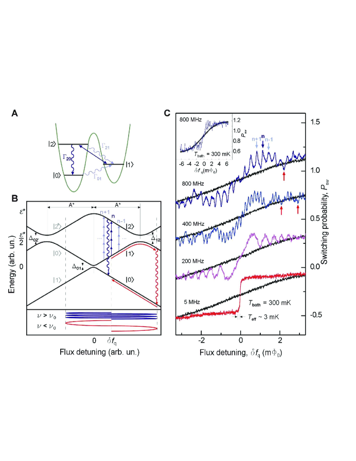
Figure 1: Sideband cooling in a flux qubit. (A) External excitation transfers the thermal population from state $|1\rangle$ to state $|2\rangle$ (straight line) from which it decays into the ground state $|0\rangle$. Wavy lines represent spontaneous relaxation and absorption, $\Gamma_{20}\gg\Gamma_{21},\Gamma_{01}$. The double well is the flux-qubit potential comprising energy levels. (B) Schematic band diagram illustrating the resonant and adiabatic sideband cooling of the ac-driven qubit. $|1\rangle\to|2\rangle$ transitions are resonant at high driving frequency $\nu$ (blue lines) and occur via adiabatic passage at low $\nu$ (red lines). $\Delta_{01}$ and $\Delta_{12}$ are the tunnel splittings between $|0\rangle$ - $|1\rangle$ and $|1\rangle$ - $|2\rangle$. (C) Cooling induced by ac-pulses with driving frequencies $\nu$ = 800, 400, 200 and 5 MHz. State $|0\rangle$ population $P_{\rm sw}$ versus flux detuning $\delta f_{\rm q}$ for the cooled qubit and for the qubit in thermal equilibrium with the bath (black lines, $T_{\rm bath}=300\,{\rm mK}$). Measurements for $\nu=$ 800, 200 and 5 MHz are displaced vertically for clarity. (Inset) $P_{\rm sw}$ versus $\delta f_{\rm q}$ over a wider range of flux detuning; $\nu=$ 800 MHz.

The cooling procedure illustrated in Fig. 1A is generalized to the energy-band diagram shown schematically in Fig. 1B. The diabatic-state energies,

$$\varepsilon_{1,0}=\pm I_{\rm q}\delta f_{\rm q},\quad\varepsilon_{2^{\prime},2}=\varepsilon^{\ast}\pm I_{\rm q}\delta f_{\rm q},$$ (1)

are linear in the flux detuning $\delta f_{\rm q}$, with the energy $\varepsilon^{\ast}\approx 25\,{\rm GHz}$ and $I_{\rm q}=1.44\,{\rm GHz/m}\Phi_{0}$ in our device, and exhibit avoided crossings $\Delta_{01}\approx 12$ MHz and $\Delta_{12}=\Delta_{02^{\prime}}\approx 100$ MHz due to quantum tunneling through the double-well barrier (Fig. 1A). The diabatic levels exchange roles at each avoided crossing, and the energy band is symmetric about $\delta f_{\rm q}=0$  (?).

Under equilibrium conditions, the average level populations exhibit a thermally-broadened “qubit step” about $\delta f_{\rm q}=0$ , the location of the $|0\rangle$ - $|1\rangle$ avoided crossing. This is determined from the switching probability $P_{\rm{sw}}$ of the measurement superconducting quantum interference device (SQUID) magnetometer, which follows the $|0\rangle$ state population  (?),

$$P_{\rm{sw}}=\frac{1}{2}(1+Fm_{0}),\quad m_{0}=\tanh\frac{\varepsilon}{2k_{B}T},$$ (2)

where $F$ is the fidelity of the measurement, $m_{0}=p_{0}-p_{1}$ is the equilibrium magnetization that results from the qubit populations $p_{0,1}$, $T=T_{\rm bath}$, and $\varepsilon=\varepsilon_{1}-\varepsilon_{0}\propto\delta f_{\rm q}$ as inferred from Eq. 1. In the presence of microwave excitation targeting the $|1\rangle\to|2\rangle$ transition, the resultant cooling, which we will later quantify in terms of an effective temperature $T_{\rm eff}<T_{\rm bath}$, acts to increase the ground-state population and, thereby, sharpen the qubit step. This cooling signature is evident in Fig. 1C, where we show the qubit step before and after applying a cooling pulse at several frequencies for $T_{\rm bath}=300$ mK.

The cooling presented in Fig. 1, B and C, exhibits a rich structure as a function of driving frequency and detuning, resulting from the manner in which state $|2\rangle$ is accessed. The $|1\rangle\to|2\rangle$ transition rate can be described by a product of a resonant factor and an oscillatory Airy factor  (?). The former dominates at high frequencies (800 and 400 MHz), where well-resolved resonances of $n$-photon transitions are observed, as illustrated in Fig. 1B (transition in blue) and Fig. 1C (top traces and inset). The cooling is thus maximized near the detuning values matching $\varepsilon_{2}-\varepsilon_{1}=nh\nu$ (downward arrows in Fig. 1C). At intermediate frequencies (400 and 200 MHz), the Airy factor becomes more prominent and accounts for the Stückelberg-like oscillations that modulate the intensity of the $n$-photon resonances  (?, ?). Below $\nu=200\,{\rm MHz}$, although individual resonances are no longer discernible, the modulation envelope persists due to the coherence of the Landau-Zener dynamics at the $\Delta_{12}$ avoided crossing  (?). The $|1\rangle\to|2\rangle$ transition becomes weak near the zeros of the modulation envelope, where we observe less efficient cooling, or even slight heating (e.g., upward arrows in Fig. 1C, 800 and 400 MHz). This is a result of the $|0\rangle\to|1\rangle$ transition rate which, although relatively small, $\Delta_{01}^{2}\ll\Delta_{12}^{2}$, acts to excite the qubit when the usually dominant $|1\rangle\to|2\rangle$ transition rate vanishes. At low frequencies [$\nu\lesssim\nu_{0}=(\Delta_{12}^{3}/A^{\ast})^{1/2}\approx 10\,{\rm MHz}$], the state $|2\rangle$ is reached via adiabatic passage (Fig. 1B, red lines) and the population transfer and cooling become conveniently independent of detuning (see $\nu=5~{}{\rm MHz}$ in Fig. 1C).

Maximal cooling occurs near an optimal driving amplitude (Fig. 2). Fig. 2A shows the $|0\rangle$ state population $P_{\rm sw}$ measured as a function of the microwave amplitude $A$ and flux detuning $\delta f_{\rm q}$ for frequency $\nu=5\,{\rm MHz}$. The adiabatic passage regime, realized at this frequency, is particularly simple to interpret, although higher frequencies allow for an analogous interpretation. Cooling and the diamond feature of size $A^{*}=\varepsilon^{*}/2I_{\rm q}$ can be understood in terms of the energy band diagram (Fig. 1B). For amplitudes $0\leq A\leq A^{*}/2$, population transfer between states $|0\rangle$ and $|1\rangle$ occurs when $A>|\delta f_{\rm q}|$, such that the sinusoidal flux reaches the $\Delta_{01}$ avoided crossing; this defines the front side of the observed spectroscopy diamond symmetric about the qubit step. For amplitudes $A^{*}/2\leq A\leq A^{*}$, the $\Delta_{12}$ ($\Delta_{02^{\prime}}$) avoided crossing dominates the dynamics, resulting in a second pair of thresholds $A=A^{*}-|\delta f_{\rm q}|$, which define the back side of the diamond. As the diamond narrows to the point $A=A^{*}$, cooling is observed. There only one of the two side avoided crossings is reached and, thereby, strong transitions with relaxation to the ground state result for all $\delta f_{\rm q}$, yielding the sharpest qubit step. For $A>A^{*}$, both side avoided crossings $\Delta_{12}$ and $\Delta_{02^{\prime}}$ are reached simultaneously when $|\delta f_{\rm q}|\lesssim A-A^{\ast}$, leading again to a large population transfer between $|0\rangle$ and $|1\rangle$.

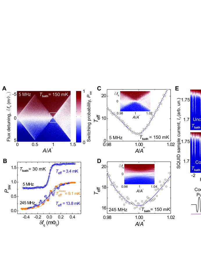
Figure 2: Optimal cooling parameters and effective temperature. (A) State $|0\rangle$ population $P_{\rm sw}$ versus flux detuning, $-A^{*}/2\lesssim\delta f_{\rm q}\lesssim A^{*}/2$, and driving amplitude $A$ with $\nu$ = 5 MHz, $t_{p}=3\,\mu{\rm s}$, and $T_{\rm bath}$ = 150 mK. Optimal conditions for cooling are realized at $A=A^{\ast}$, where $A^{*}$ is defined in Fig. 1B. (B) Effective temperature $T_{\rm{eff}}$. Qubit steps measured at $\nu=$ 5 and 245 MHz (circles) and best fits to Eq. 2. At 245 MHz, the aggregate temperature fitting (blue, $T_{\rm{eff}}$ = 13.8 mK) and the convex fitting (orange, $T_{\rm{eff}}$ = 9.1 mK) are shown. $T_{\rm bath}$ = 30 mK. (C and D) (Inset) Detail of the region $A\approx A^{*}$ [white box in (A)] for $\nu$ = 5 MHz (top) and $\nu$ = 245 MHz (bottom). In each case, $T_{\rm{eff}}$ is extracted from the qubit step as in (B). Lines are guides for the eye; $t_{\rm p}=3~{}\mu$s, $T_{\rm bath}$ = 150 mK. (E) Spectroscopy of uncooled (top) and cooled (middle) qubit (5 MHz, 3-$\mu$s cooling pulse) at $T_{\rm bath}=30$ mK. Cumulative switching-probability distribution as a function of $I_{\rm{s}}$ and $\delta f_{\rm{q}}$ under 500-MHz ac excitation.

When an ac field is applied, the qubit is no longer in equilibrium with the bath, but it can still be well-characterized by an effective temperature $T_{\rm{eff}}$ using Eq. 2 with $T=T_{\rm{eff}}$. This is illustrated in Fig. 2B for $\nu=5$ MHz and $\nu=245$ MHz ($T_{\rm{bath}}=30$ mK). At $\nu=5$ MHz, the qubit step clearly follows Eq. 2, as shown with a fit line for $T_{\rm{eff}}=3.4$ mK. At 245 MHz, individual multiphoton resonances are evident, and $P_{\rm{sw}}$ is a non-monotonic function of $\delta f_{\rm{q}}$. In this case, $T_{\rm{eff}}$ is still a useful parameter to quantify the effective cooling, but it should be interpreted as an aggregate temperature over all frustrations. Alternatively, because the cooling is maximized at individual resonances, one may perform a convex fitting of Eq. 2, where only the solid (orange) symbols are taken into account to determine the effective temperature at the resonance detunings. The convex effective temperature $T_{\rm{eff}}^{\rm convex}=9.1$ mK is smaller than the aggregate value $T_{\rm{eff}}=13.8$ mK. In the remainder of the paper, we refer to the more conservative effective temperature obtained using the aggregate definition.

Figure 2, C and D, show the variation of $T_{\rm eff}$ about $A=A^{*}$ for $\nu=5$ MHz and $\nu=245$ MHz, respectively, in the region marked with a white rectangle in Fig. 2A (insets show the raw data). As seen in these figures, $T_{\rm eff}$ typically presents a minimum, where the cooling is most efficient and from which $A^{*}$ can be determined.

To determine whether the observation of a sharp qubit step proves that the system makes transitions to the ground state, as opposed to selectively populating an excited state with the same magnetization, we measured the excitation spectra of the “pre-cooled” qubit and of the qubit in thermal equilibrium with the bath (Fig. 2E). In the former, a weak ac excitation was applied immediately after the cooling pulse (time-lag less than 100 ns), well before the system equilibrates by warming up to the bath temperature (see below). By comparing the excitation spectra of the equilibrium and cooled systems (Fig. 2E, $T_{\rm bath}=30$ mK), we note that, although cooling markedly reduces the step width, making the qubit much colder, the excitation spectrum remains unchanged. Because the ac excitation is resonant with the $|0\rangle\to|1\rangle$ transition only, this strongly indicates that the population in a cooled qubit is in the ground state.

Figure 3, A and B, summarize the dependence of $T_{\rm{eff}}^{*}=T_{\rm{eff}}(A^{*})$ on the dilution refrigerator temperature $T_{\rm{bath}}=30-400$ mK for several frequencies $\nu$, spanning the resonant sideband to the adiabatic passage limits, with a fixed pulse width $t_{\rm p}=3~{}\mu$s. In Fig. 3A, at large $\nu$, $T_{\rm{eff}}^{*}$ exhibits a monotonic increase with $T_{\rm{bath}}$, which becomes less pronounced as $\nu$ decreases. In the adiabatic passage limit, e.g. $\nu=5$ MHz, $T_{\rm{eff}}^{*}\approx 3$ mK is practically constant and reaches values that, notably, can be more than two orders of magnitude smaller than $T_{\rm{bath}}$. In Fig. 3B, $T_{\rm eff}^{*}$ is observed to increase linearly with $\nu$ for different values of $T_{\rm bath}$. Because the number of resonances in the qubit-step region is inversely proportional to $\nu$, the cooling at the individual resonances depends only weakly on $\nu$ when using the convex definition $T_{\rm{eff}}^{\rm convex}(A^{*})$.

Figure 3C displays the measurement-fidelity $F$ versus $T_{\rm{bath}}$. Although the qubit is effectively cooled, $T_{\rm eff}^{*}\ll T_{\rm{bath}}$, over the range of $T_{\rm{bath}}$ in Fig. 3, A and B, the readout SQUID is not actively cooled, and its switching current distribution broadens with $T_{\rm{bath}}$ (fig. S2). At high temperatures, the fidelity $F$, defined in Eq. 2, becomes too small to discriminate the two qubit states; this is independent of the qubit’s effective temperature, which remains $\sim$3 mK at all values of $T_{\rm{bath}}$. We observe that the fidelity $F$ is larger than 0.8 for $T_{\rm{bath}}<100$ mK, remains above 0.5 at ³He refrigerator temperatures, but drops to $F\approx 0.1$ at $T_{\rm{bath}}=400$ mK, limiting our ability to measure the qubit state at higher temperatures (SOM Text).

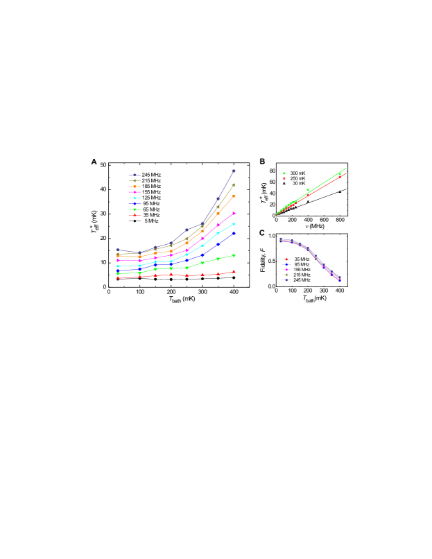
Figure 3: Effective temperature $T_{\rm eff}^{*}$ for $A=A^{*}$ and measurement fidelity $F$. (A) $T_{\rm eff}^{*}$ versus $T_{\rm{bath}}$ at the indicated driving frequencies $\nu$. $T_{\rm eff}^{*}$ increases with $T_{\rm{bath}}$ at high $\nu$, but remains constant at low $\nu$. (B) $T_{\rm eff}^{*}$ versus $\nu$ for different $T_{\rm{bath}}$. Lines are linear fits. (C) $F$ versus $T_{\rm{bath}}$ at the indicated $\nu$. A pulse width $t_{\rm p}=3~{}\mu$s was used in all cases.

The cooling and equilibration dynamics of the qubit are summarized in Fig. 4 ($T_{\rm bath}=150$ mK). Cooling a qubit in equilibrium with the bath requires a characteristic cooling time. In turn, a cooled qubit is effectively colder than its environment, a non-equilibrium condition, which over a characteristic equilibration time will thermalize to the environmental bath temperature. This relation between cooling and equilibration times determines the facility of cooling the qubit and performing operations while still cold. Fig. 4, A and B, show the time evolution at cooling and warming up of the qubit step. The top panels show $P_{\rm sw}$ as a function of $\delta f_{\rm q}$ and cooling-pulse length $t_{\rm p}$ (Fig. 4A, $\nu=245$ MHz), and as a function of $\delta f_{\rm q}$ and waiting-time $t_{\rm w}$ after pre-cooling with a 5 MHz pulse (Fig. 4B) (for $t_{\rm p}$ and $t_{\rm w}$ definition, see fig. S1). Note the difference in the time scales, where it is observed that substantial cooling is accomplished within 1 $\mu$s (Fig. 4A), but equilibration occurs over a much longer time scale (Fig. 4B). Fitting to Eq. 2 yields $T_{\rm eff}$ as a function of $t_{\rm p}$ and $t_{\rm w}$ (Fig. 4, A and B, bottom panels). The near exponential behavior of $T_{\rm eff}$ versus $t_{\rm p}$ and $t_{\rm w}$ allows one to infer the characteristic cooling and equilibration times as defined by an exponential fitting (solid blue lines), which are summarized in Fig. 4C. Notably, the cooling characteristic time is nearly independent of both $\nu$ and $T_{\rm bath}$ and, on average, is about 500 ns. In contrast, at the base temperature of the dilution refrigerator, the equilibration time is about three orders of magnitude longer, 300 $\mu$s, and remains one order of magnitude longer at 250 mK, a temperature that is accessible with ³He refrigerators.

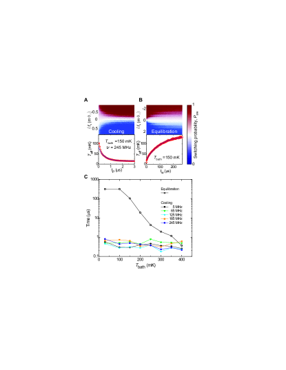
Figure 4: Dynamics of cooling and equilibration. (A) (Upper panel) State $|0\rangle$ population $P_{\rm sw}$ as a function of $\delta f_{\rm q}$ and cooling pulse width $t_{\rm p}$ ($\nu$ = 245 MHz). (Lower panel) $T_{\rm{eff}}$ versus $t_{\rm p}$ extracted from upper panel (circles) and exponential fit (blue line) with $\sim$ 1-$\mu$s time constant. (B) (Upper panel) State $|0\rangle$ population $P_{\rm sw}$ as a function of $\delta f_{\rm q}$ and waiting time $t_{\rm w}$ after the cooling pulse ($t_{\rm p}=3~{}\mu$s and $\nu=$ 5 MHz). (Lower panel) $T_{\rm{eff}}$ versus $t_{\rm w}$ extracted from upper panel (circles) and exponential fit (blue line) with $\sim$ 100-$\mu$s time constant. $T_{\rm{bath}}$ = 150 mK. (C) Characteristic equilibration and cooling times for different $T_{\rm{bath}}$. Cooling is performed at the indicated frequencies.

The minimum qubit effective temperature demonstrated in this work was estimated to be $T_{\rm eff}\approx 3$ mK. This value is consistent with the inhomogeneously broadened linewidth observed in the experiment, which likely places a lower limit on the measurable minimum temperature. The microwave-induced cooling presented here can be applied to problems in quantum information science, including ancilla-qubit reset for quantum error correcting codes and quantum-state preparation, with implications for improved fidelity and decoherence in multi-qubit systems. This approach, realized in a superconducting qubit, is generalizable to other solid-state qubits and can be used to cool other on-chip elements, e.g. the qubit circutry or resonators

• We thank A. J. Kerman, D. Kleppner, and A. V. Shytov for helpful discussions; and V. Bolkhovsky, G. Fitch, D. Landers, E. Macedo, P. Murphy, R. Slattery, and T. Weir at MIT Lincoln Laboratory for technical assistance. This work was supported by Air Force Office of Scientific Research (grant F49620-01-1-0457) under the DURINT program and partially by the Laboratory for Physical Sciences. The work at Lincoln Laboratory was sponsored by the US Department of Defense under Air Force Contract No. FA8721-05-C-0002.

Materials and Methods

Measurement Scheme

The qubit consists of a superconducting loop interrupted by three Josephson junctions (Fig. S5A), one of which has a reduced cross-sectional area. DC and pulsed microwave (MW) magnetic fields generate a time-dependent magnetic flux $f(t)=f^{\rm dc}+f^{\rm ac}(t)$ threading the qubit. Transitions between the qubit states are driven by the pulsed MW flux $f^{\rm ac}(t)=A\cos 2\pi\nu t$ of duration $t_{\rm p}=10\,{\rm ns}-3\,\mu{\rm s}$ (Fig. S5B) with frequency $\nu$, and amplitude $A$, where $A$ is proportional to the MW-source voltage $V_{\rm ac}$. The qubit states are read out using a DC-SQUID, a sensitive magnetometer that distinguishes the flux generated by the qubit persistent currents, $I_{\rm q}$. After a delay $t_{\rm w}$ following the excitation, the readout is performed by driving the SQUID with a 20-ns “sample” current $I_{\rm{s}}$ followed by a 20-$\mu$s “hold” current (Fig. S5B). The SQUID will switch to its normal state voltage $V_{\rm{s}}$ if $I_{\rm{s}}>I_{\rm{sw,0}}$ ($I_{\rm{s}}>I_{\rm{sw,1}}$), when the qubit is in state $|0\rangle$ ($|1\rangle$). By sweeping $I_{\rm{s}}$ and flux detuning, while monitoring the presence of a SQUID voltage over many trials, we generate a cumulative switching distribution function (see Fig. 2E and Fig. S2 below). By following a flux-dependent sample current $I_{\rm{sw,0}}<I_{\rm{s}}<I_{\rm{sw,1}}$ we obtain the switching probability $P_{\rm{sw}}$ that characterizes the population of state $|0\rangle$, and that reveals the “qubit step” shown in Fig. 1C.

The experiments were performed in a dilution refrigerator with a 12-mK base temperature. The device was magnetically shielded with 4 Cryoperm-10 cylinders and a superconducting enclosure. All electrical leads were attenuated and/or filtered to minimize noise.

Device Fabrication and Parameters

The device (Fig. S5A) was fabricated at MIT Lincoln Laboratory on 150 mm wafers in a fully-planarized niobium trilayer process with critical current density $J_{\rm{c}}\approx 160$ $\rm{A}/\rm{cm}^{2}$. The qubit’s characteristic Josephson and charging energies are $E_{\rm{J}}\approx(2\pi\hbar)300$ GHz and $E_{\rm{C}}\approx(2\pi\hbar)0.65$ GHz respectively, the ratio of the qubit Josephson junction areas is $\alpha\approx 0.84$, and the tunnel coupling $\Delta\approx(2\pi\hbar)0.01$ GHz. The qubit loop area is 16 $\times$ 16 $\mu$m², and its self inductance is $L_{\rm{q}}\approx 30$ pH. The SQUID Josephson junctions each have critical current $I_{\rm{c0}}\approx 2$ $\mu$A. The SQUID loop area is 20 $\times$ 20 $\mu$m², and its self inductance is $L_{\rm{S}}\approx 30$ pH. The mutual coupling between the qubit and the SQUID is $M\approx 25$ pH.

Supporting Text

Microwave cooling and optical resolved sideband cooling

While the microwave cooling (MC) demonstrated in this work has similarities with optical resolved sideband cooling (RSC), the analogy is not a tautology. We describe here the similarities and distinctions between the two cooling techniques.

In both cases, the spectra of the energy levels can be reduced to the three-level system defined in Fig. 1A (main text). Although, as described below, the origin of the three levels is different for MC and RSC, cooling is similarly achieved by driving the thermal population in state $|1\rangle$ to an ancillary state $|2\rangle$, from which it quickly relaxes to state $|0\rangle$.

In the case of RSC of an atom, the three-level system illustrated in Fig. 1A (without the double-well potential) results from a two-level atomic system (TLS) combined with a simple harmonic oscillator (SHO) from the trap potential. Using the notation $|\text{TLS state},\text{SHO state}\rangle$ with TLS states $\{|g\rangle,|e\rangle\}$ and SHO states $\{|n\rangle\}$ with $n=0,1,2,\ldots$, one can identify from Fig. 1A the following: $|0\rangle_{\text{RSC}}\equiv|g,n\rangle$, $|1\rangle_{\text{RSC}}\equiv|g,n+1\rangle$, and $|2\rangle_{\text{RSC}}\equiv|e,n\rangle$. Note that the TLS represents an “internal” atomic state, whereas the SHO is an “external” trap state.

In the case of MC of a flux qubit, the double-well potential illustrated in Fig. 1A comprises two coupled SHO-like wells. The left and right wells correspond to the diabatic states of the qubit, the clockwise and counterclockwise circulating currents, and together form the qubit TLS. Each well independently has a series of SHO-like states. Using the same notation $|\text{TLS state},\text{SHO state}\rangle$ with TLS states $\{|g\rangle,|e\rangle\}$, associated respectively to the left and right well in Fig. 1A, one can identify the following: $|0\rangle_{\text{MC}}\equiv|g,0\rangle$, $|1\rangle_{\text{MC}}\equiv|e,0\rangle$, and $|2\rangle_{\text{MC}}\equiv|g,1\rangle$. Further higher-excited states are not explicitly shown in Fig. 1A. Note that all states here are “internal,” and that the SHO-nature of the left and right wells is limited by the degree of tunnel coupling between wells.

From the above discussion, it is clear that in both RSC and MC there is a TLS combined with a SHO, however the roles of the levels interchange. Considering an associated frequency $\omega_{\text{TLS}}=E_{\text{TLS}}/\hbar$ for the TLS and a plasma frequency $\omega_{\text{SHO}}=E_{\text{SHO}}/\hbar$, the two cases can be summarized as follows:

• In the RSC case, $\omega_{\text{SHO}}<\omega_{\text{TLS}}$, and it is the SHO that is cooled. One drives population from the TLS ground state with higher SHO energy, $|1\rangle_{\text{RSC}}\equiv|g,n+1\rangle$, to the TLS excited-state with lower SHO energy, $|2\rangle_{\text{RSC}}\equiv|e,n\rangle$, from which it relaxes to the ground state $|0\rangle_{\text{RSC}}\equiv|g,n\rangle$.

• In the MC case, $\omega_{\text{TLS}}<\omega_{\text{SHO}}$, and it is the TLS that is cooled. One drives population from the TLS excited state with low SHO energy, $|1\rangle_{\text{MC}}\equiv|e,0\rangle$, to the TLS ground-state with higher SHO energy, $|2\rangle_{\text{RSC}}\equiv|g,1\rangle$, from which it relaxes to the ground state $|0\rangle_{\text{MC}}\equiv|g,0\rangle$.

Thus, if one considers a three-level state configuration without tagging the states with the terms “external” or “internal”, in one cooling cycle, one cools the subsystem of interest $\{|0\rangle,|1\rangle\}$ by driving transitions to an ancillary state $|2\rangle$, which relaxes quickly to the ground state. For MC, the cooled subsystem is the TLS, whereas for RSC, the cooled subsystem is the SHO. Note that in the RSC case, because it is the SHO that is cooled, the cooling cycles can be cascaded to cool the multiple SHO states $n=0,1,2,\ldots$. However, in the MC case, it is the TLS that is cooled, which requires only a single cooling cycle from the TLS excited state to its ground state. In the MC case described in this work, all transitions are allowed, and the energy levels are widely tunable. However, in many cases of RSC of atoms, certain transitions may be forbidden, and there is typically only limited energy-band tunability.

Effective temperature and fidelity vs. bath temperature

The qubit step and the SQUID switching-current distribution broaden with $T_{\rm{bath}}$. The qubit can be cooled effectively, $T_{\rm eff}^{*}\ll T_{\rm{bath}}$, over the range of $T_{\rm{bath}}$ in Fig. 3A and Fig. 3B. However, the readout SQUID is not actively cooled, and its switching current distribution broadens with $T_{\rm{bath}}$. This is observed in Fig. S6, where we plot the cumulative switching-distribution as a function of $I_{\rm s}$ and $\delta f_{\rm q}$ of uncooled and cooled qubit (5 MHz, 3-$\mu$s cooling pulse) at different $T_{\rm bath}$. At high temperatures, the switching-current distribution becomes broad and the measurement fidelity $F$ drops to values that become too small to discriminate the two qubit states; this is independent of the qubit’s effective temperature, which remains about 3 mK at all $T_{\rm{bath}}$.

Supporting Figures

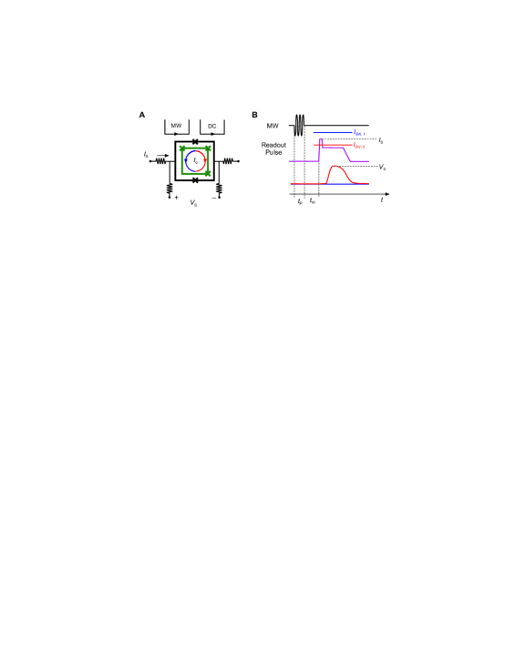
Figure 5: (Fig. S1) Schematic flux qubit and measurement scheme. (A) Qubit (inner green loop) and inductively coupled DC SQUID magnetometer (outer black loop). Josephson junctions are indicated by crosses. Red and blue arrows indicate the two directions of the persistent current in the qubit, $I_{\rm q}$. DC and pulsed MW magnetic fields $f(t)=f^{\rm dc}+f^{\rm ac}(t)$ control the qubit and drive transitions between its quantum states. (B) The qubit state is inferred by sampling the SQUID with a pulsed current $I_{\mathrm{s}}$ and performing voltage readout of the switching pulse, $V_{\mathrm{s}}$. The current pulse $I_{\mathrm{s}}$ is set to maximize the difference in the SQUID switching probability between the two qubit states which couple to the SQUID through the associated persistent currents, $I_{\rm q}$. The SQUID only switches when the qubit is in state $|0\rangle$ and the switching probability $P_{\rm sw}$ measures its population.

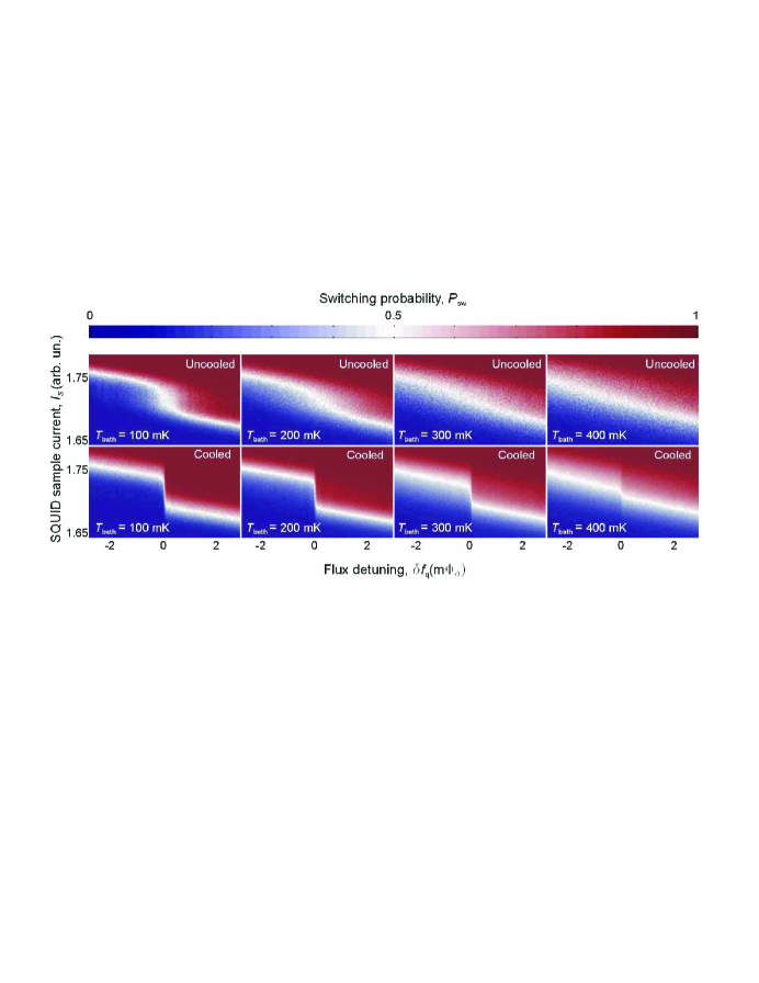
Figure 6: (Fig. S2) Cumulative switching distribution of the qubit as a function of $I_{\rm{s}}$ and $\delta f_{\rm{q}}$ of the qubit in equilibrium with the bath (top) and of the cooled qubit (bottom) at different $T_{\rm bath}$. The cooling pulse $t_{\rm p}=3~{}\mu$s, $\nu$ = 5 MHz. Although the readout SQUID switching distribution broadens as $T_{\rm bath}$ increases, reducing the readout fidelity, the cooled qubit step remains sharp $(T_{\rm eff}\sim 3$ mK).

References and Notes

- 1. S. Chu, Rev. Mod. Phys. 70, 685 (1998).
- 2. C. N. Cohen-Tannoudji, Rev. Mod. Phys. 70, 707 (1998).
- 3. W. D. Phillips, Rev. Mod. Phys. 70, 721 (1998).
- 4. D. Leibfried, R. Blatt, C. Monroe, D. Wineland, Rev. Mod. Phys. 75, 281 (2003).
- 5. D. J. Wineland, R. E. Drullinger, F. L. Walls, Phys. Rev. Lett. 40, 1639 (1978).
- 6. W. Neuhauser, M. Hohenstatt, P. Toschek, H. Dehmelt, Phys. Rev. Lett. 41, 233 (1978).
- 7. I. Marzoli, J. I. Cirac, R. Blatt, P. Zoller, Phys. Rev. A 49, 2771 (1994).
- 8. C. Monroe et al., Phys. Rev. Lett. 75, 4011 (1995).
- 9. H. Perrin, A. Kuhn, I. Bouchoule, C. Salomon, Europhys. Lett, 42, 395 (1998).
- 10. V. Vuletić, C. Chin, A. J. Kerman, S. Chu, Phys. Rev. Lett. 81, 5768 (1998).
- 11. A. J. Kerman, V. Vuletić, C. Chin, S. Chu, Phys. Rev. Lett. 84, 439 (2000).
- 12. G. Morigi, J. Eschner, C. H. Keitel, Phys. Rev. Lett. 85, 4458 (2000).
- 13. C. E. Wieman, D. E. Pritchard, D. J. Wineland, Rev. Mod. Phys. 71, S253 (1999).
- 14. J. Clarke, A. N. Cleland, M. H. Devoret, D. Esteve, J. H. Martinis, Science 239, 992 (1988).
- 15. Y. Makhlin, G. Schön, A. Shnirman, Rev. Mod. Phys. 73, 357 (2001).
- 16. J. R. Friedman, V. Patel, W. Chen, S. K. Tolpygo, J. E. Lukens, Nature 406, 43 (2000).
- 17. C. H. van der Wal et al., Science 290, 773 (2000).
- 18. Y. Nakamura, Y. A. Pashkin, J. S. Tsai, Nature 398, 786 (1999).
- 19. Y. Nakamura, Y. A. Pashkin, J. S. Tsai, Phys. Rev. Lett. 87, 246601 (2001).
- 20. D. Vion et al. Science 296, 886 (2002).
- 21. Y. Yu, S. Han, X. Chu, S.-I. Chu, Z. Wang, Science 296, 889 (2002).
- 22. J. M. Martinis, S. Nam, J. Aumentado, C. Urbina, Phys. Rev. Lett. 89, 117901 (2002).
- 23. I. Chiorescu, Y. Nakamura, C. J. P. M. Harmans, J. E. Mooij, Science 299, 1869 (2003).
- 24. S. Saito et al., Phys. Rev. Lett. 96, 107001 (2006)
- 25. I. Chiorescu et al., Nature 431, 159 (2004).
- 26. A. Wallraff et al., Nature 431, 162 (2004).
- 27. J. Johansson et al., Phys. Rev. Lett. 96, 127006 (2006).
- 28. W. D. Oliver et al., Science 310, 1653 (2005).
- 29. M. Sillanpää, T. Lehtinen, A. Paila, Yu. Makhlin, P. Hakonen, Phys. Rev. Lett. 96, 187002 (2006).
- 30. D.M. Berns et al., Phys. Rev. Lett. 97, 150502 (2006), cond-mat/0606271.
- 31. T. P. Orlando et al., Phys. Rev. B 60, 15398 (1999).
- 32. Materials and methods are available as supporting material on Science Online.
- 33. For negative , levels and exchange roles, and level plays the role of level . Unless explicitly noted, the discussions herein refer to positive .
-
1.