From tunneling to contact: Inelastic signals in an atomic gold junction

Abstract

The evolution of electron conductance in the presence of inelastic effects is studied as an atomic gold contact is formed evolving from a low-conductance regime (tunneling) to a high-conductance regime (contact). In order to characterize each regime, we perform density functional theory (DFT) calculations to study the geometric and electronic structures, together with the strength of the atomic bonds and the associated vibrational frequencies. The conductance is calculated by first evaluating the transmission of electrons through the system, and secondly by calculating the conductance change due to the excitation of vibrations. As found in previous studies [Paulsson et al., Phys. Rev. B. 72, 201101(R) (2005)] the change in conductance due to inelastic effects permits to characterize the crossover from tunneling to contact. The most notorious effect being the crossover from an increase in conductance in the tunneling regime to a decrease in conductance in the contact regime when the bias voltage matches a vibrational threshold. Our DFT-based calculations actually show that the effect of vibrational modes in electron conductance is rather complex, in particular when modes localized in the contact region are permitted to extend into the electrodes. As an example, we find that certain modes can give rise to decreases in conductance when in the tunneling regime, opposite to the above mentioned result. Whereas details in the inelastic spectrum depend on the size of the vibrational region, we show that the overall change in conductance is quantitatively well approximated by the simplest calculation where only the apex atoms are allowed to vibrate. Our study is completed by the application of a simplified model where the relevant parameters are obtained from the above DFT-based calculations.

I Introduction

Recent experimental advances have permitted to probe electron transport processes at the atomic scale.Agrait:2003 Junctions can be formed that support current flow through atom-sized constrictions or even single molecules. Atomic vibrations become detectable and very dependable on the environmental temperature. According to the distance between electrodes, the conductance can vary several orders of magnitude when the applied voltages are small, typically below the eV scale. This behavior is due to the exponential dependence of current with distance when the conductance is due to an electron tunneling process. However, at short electrode distances, the current levels off and saturates: the contact regime is reached. The conductance is maximum in this case and a high-conductance regime is attained. The physics in these two regimes can be very different.

The low-conductance regime has been thoroughly studied with the scanning tunneling microscope (STM). The initial inelastic effects were realized by showing the increase in conductance on an acetylene molecule when the bias voltage matched the C–H stretch mode.Stipe:1998 The proof that the mode was indeed excited was the isotopical effect that the changes of conductance showed when replacing C₂H₂ by C₂D₂. This finding paved the way to vibrational spectroscopy with sub-Ångström spatial resolution, permitting the identification of chemical components of matter on the atomic scale.Pascual:2005 ; Komeda:2005 The first experimental evidence of mode excitation in the high-conductance regime was achieved in monatomic gold wires.Agrait:2002 The conductance of the wires showed clear reductions at thresholds that were proven to originate in the backscattering of electrons from some selected vibrations of the wires.Agrait:2002 ; Frederiksen:2004 Similarly, experiments with the break junction geometry have also revealed signatures in the conductance related to several vibrational modes of a single H₂ molecule trapped between the electrodes.Smit:2002

The emerging picture is that in the tunneling or low-conductance regime, the excitation of vibrations leads to increases in conductance at the corresponding voltage thresholds, while in the contact or high-conductance regime, the effect of vibrations is to reduce the conductance. Theoretical studies in the weak electron-vibration coupling regime have shown that the lowest order expansionGalperin:2004 is capable of correlating this behavior with a single parameter: the eigenchannel transmission probability $\tau$.Paulsson:2005 ; Viljas:2005 ; delaVega:2006 In the simplified case of a single electronic level connected with two electrodes under symmetrical conditions, the inelastic effects (of a vibrationally mediated on-site modulation) go from increases in the conductance for $\tau<1/2$ to decreases for $\tau>1/2$. In this way, the behavior of the inelastic conductance would define the crossover from tunneling to contact. There is experimental evidence showing that this picture is indeed more complex. The excitation of the O–O stretch mode of the chemisorbed O₂ molecule on Ag(110) Hahn:2000 leads to a decrease of the tunneling current (instead of an increase) in opposition with most cases in the low-conductance regime.Persson:1984 ; Lorente:2004

The aim of the present work is to analyze the continuous evolution from tunneling to contact in a model system constituted by a junction of gold atoms, which provides an almost perfect realization of a single transmission channel system. The definition of when a given atomic system correspond to one of the two cases analyzed above is already problematic, hence we address this issue by investigating the behavior of different properties of the junction with the interatomic distance. Initially, we are interested in studying the crossover from tunneling to contact by evaluating the total energy, the strain, and the modification of vibrational modes as the electrode distance decreases. This allows us to find a range of distances where the junction behaves as either two independent systems or a strongly coupled one. The second part of this work evaluates the effect of the interatomic distance in electron transmission; this allows us to study the elastic conductance within Landauer’s formalism. The correlation of the transmission against the interatomic relaxation permits a clear identification of both regimes as well as the transition region. Finally, the inelastic properties of the conductance are studied in the different regimes. The inelastic signals are interpreted in a simplified model that captures the calculated behavior and illustrates the fundamental concepts.

The continuous transition from tunneling to contact is experimentally challenging, since most metallic point contacts (including Au) usually exhibits a sudden jump in the conductance when the surfaces are brought into contact.Untiedt:2006 On the other hand, experiments with a low-temperature STM on Cu(111) and Ag(111) surfaces have shown that both sharp jumps as well as smooth variations can be obtained in the crossover from tunneling to contact: when the tip is approached over a clean surface one observes a jump in conductance (related to the transfer of the tip-atom to the surface), whereas over an isolated metallic adatom the evolution is smooth and reversible.Limot:2005 To our knowledge there is no measurement of the evolution of the inelastic signals in the formation of a metallic point contact, likely owing the relative weak effect (conductance changes expected to be less than 1%) and difficulties with noise. Despite this we envision that our idealized model system is not unrealistic, and can provide a useful framework for investigating the complicated interplay between chemical bonding, electron conduction, atomic vibrations, etc. Our first-principles treatment further addresses all of these issues in a unified way to provide quantitative predictions.

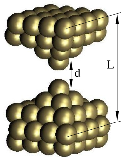
Figure 1: (Color online) Generic setup for the calculation of structural properties of the atomic gold junction. The periodic supercell consists of a $4\times 4$ representation of two Au(100) surfaces sandwiching two pyramids pointing towards each other. The characteristic electrode separation $L$ is measured between the second-topmost surface layers, since the surface layer itself is relaxed and hence deviates on the decimals from the bulk values. The interatomic distance between the apex atoms is denoted $d$.

II Theory

The present work can be divided by the different methods that we have used. In order to study the structural properties of the atomic junction the standard DFT SiestaSoler:2002 method is used. The elastic conductance is evaluated from the transmission function of the atomic junction calculated with TranSiesta,Brandbyge:2002 and the inelastic contribution is performed using the method presented in Ref. [Paulsson:2005, ; Frederiksen:2006, ].

The system representing the atomic junction is depicted in Fig. 1. We consider a periodic supercell with a $4\times 4$ representation of two Au(100) surfaces sandwiching two pyramids pointing towards each other. The characteristic electrode separation $L$ will be measured between the second-topmost surface layers, since the surface layer itself is relaxed and hence deviates on the decimals from the bulk values. The corresponding calculations with the Siesta method are carried out using a single zeta plus polarization (SZP) basis with a confining energy of 0.01 Ry (corresponding to the 5$d$ and 6$(s,p)$ states of a free Au atom), the generalized gradient approximation (GGA) for the exchange-correlation functional, a cutoff energy of 200 Ry for the real-space grid integrations, and the $\Gamma$-point approximation for the sampling of the three-dimensional Brillouin zone. The interaction between the valence electrons and the ionic cores are described by a standard norm-conserving Troullier-Martins pseudo-potential generated from a relativistic atomic calculation.

The calculations of the vibrations are performed by diagonalization of the dynamical matrix extracted from finite differences (with corrections for the egg-box effect, i.e., the movement of basis orbitals—following the displaced atoms—with respect to the real space integration grid).Frederiksen:2006 As the active atoms we consider initially—for pedagogical purposes—just the two apex atoms and compare afterwards the results when the vibrational region is enlarged.

The transport calculation naturally considers infinite electrodes by including the DFT self-energy calculated for infinite atomistic leads in the conduction equations.Brandbyge:2002 Since we are here interested in the low-bias regime (of the order of the vibrational frequencies) it suffices to calculate the electronic structure in equilibrium in order to describe the elastic transport properties. While the transmission generally involves a sampling over $\mathbf{k}$-points we here approximate it with its $\Gamma$-point value; this has previously been shown to be a reasonable approximation for supercells of similar dimensions in the case of atomic gold wires.Frederiksen:2006

Finally, the inelastic transport calculations are performed using the nonequilibrium Green’s function (NEGF) formalism combined with the electrode couplings $\mathbf{\Gamma}_{L,R}$ extracted from the TranSiesta calculations and the electron-vibration couplings $\mathbf{M}^{\lambda}$ (corresponding to modes $\lambda$ with energies $\hbar\omega_{\lambda}$) from the finite-difference method.Frederiksen:2006 According to the lowest order expansion (LOE)Paulsson:2005 ; Viljas:2005 the inelastic current reads

$$I^{\mathrm{LOE}} = \textrm{G}_{0}V\mathrm{Tr}[\mathbf{G}\mathbf{\Gamma}_{R}\mathbf{G}^{\dagger}\mathbf{\Gamma}_{L}]$$ (1)

$$+\sum_{\lambda}{\cal I}^{\mathrm{sym}}_{\lambda}(V,T,\langle n_{\lambda}\rangle)\,\mathrm{Tr}\Big{[}\mathbf{G}^{\dagger}\mathbf{\Gamma}_{L}\mathbf{G}\Big{\{}\mathbf{M}^{\lambda}\mathbf{A}_{R}\mathbf{M}^{\lambda}+\frac{i}{2}(\mathbf{\Gamma}_{R}\mathbf{G}^{\dagger}\mathbf{M}^{\lambda}\mathbf{A}\mathbf{M}^{\lambda}-\mathrm{h.c.})\Big{\}}\Big{]}$$

$$+\sum_{\lambda}{\cal I}^{\mathrm{asym}}_{\lambda}(V,T)\,\mathrm{Tr}\Big{[}\mathbf{G}^{\dagger}\mathbf{\Gamma}_{L}\mathbf{G}\Big{\{}\mathbf{\Gamma}_{R}\mathbf{G}^{\dagger}\mathbf{M}^{\lambda}(\mathbf{A}_{R}-\mathbf{A}_{L})\mathbf{M}^{\lambda}+\mathrm{h.c.}\Big{\}}\Big{]},$$

$${\cal I}^{\mathrm{sym}}_{\lambda} = \frac{e}{\pi\hbar}\left({2eV}\langle n_{\lambda}\rangle+\frac{\hbar\omega_{\lambda}-{eV}}{e^{\beta(\hbar\omega_{\lambda}-eV)}-1}-\frac{{\hbar\omega_{\lambda}}+{eV}}{e^{\beta(\hbar\omega_{\lambda}+eV)}-1}\right),$$ (2)

$${\cal I}^{\mathrm{asym}}_{\lambda} = \frac{e}{\hbar}\int_{-\infty}^{\infty}\frac{d\varepsilon}{2\pi}\left[n_{\textrm{F}}(\varepsilon)-n_{\textrm{F}}(\varepsilon-eV)\right]\,{\cal H}_{\varepsilon^{\prime}}\{{n_{\textrm{F}}(\varepsilon^{\prime}+\hbar\omega_{\lambda})-n_{\textrm{F}}(\varepsilon^{\prime}-\hbar\omega_{\lambda})}\}(\varepsilon),$$ (3)

where G${}_{0}=2e^{2}/$h is the conductance quantum, $V$ the external bias voltage, $\langle n_{\lambda}\rangle$ the occupation of mode $\lambda$, $n_{\textrm{F}}(\varepsilon)$ the Fermi function, ${\cal H}$ the Hilbert transform, and $\beta=1/\textrm{k}_{B}T$ the inverse temperature. The retarded Green’s function $\mathbf{G}$, the spectral function $\mathbf{A}=i(\mathbf{G}-\mathbf{G}^{\dagger})$, as well as the electrode couplings $\mathbf{\Gamma}_{L,R}$ are all evaluated at the Fermi energy in the LOE scheme. For convenience we have also defined the quantities $\mathbf{A}_{L,R}=\mathbf{G}\mathbf{\Gamma}_{L,R}\mathbf{G}^{\dagger}$ such that $\mathbf{A}=\mathbf{A}_{L}+\mathbf{A}_{R}$. The sums in Eq. (1) runs over all modes $\lambda$ in the vibrational region. For a symmetric system (such as the present one for the atomic junction) it can be shown that the asymmetric terms in the current expression vanishes. Furthermore, at low temperatures ($\beta\rightarrow\infty$) and in the externally damped limit ($\langle n_{\lambda}\rangle\approx 0$) the inelastic conductance change from each mode $\lambda$ (beyond the threshold voltage $eV>\hbar\omega_{\lambda}$) is given by

$$\delta G_{\lambda} = \mathrm{G}_{0}\,\mathrm{Tr}\Big{[}\mathbf{G}^{\dagger}\mathbf{\Gamma}_{L}\mathbf{G}\Big{\{}\mathbf{M}^{\lambda}\mathbf{G}\mathbf{\Gamma}_{R}\mathbf{G}^{\dagger}\mathbf{M}^{\lambda}+\frac{i}{2}(\mathbf{\Gamma}_{R}\mathbf{G}^{\dagger}\mathbf{M}^{\lambda}\mathbf{A}\mathbf{M}^{\lambda}-\mathrm{h.c.})\Big{\}}\Big{]}.$$ (4)

From this expression we note that $\delta G_{\lambda}$ can be either positive or negative, depending on sign of the trace.

III Structural and vibrational properties of the atomic junction

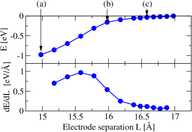
Figure 2: (Color online) Total energy differences and the numerical derivatives as a function of the electrode separation. The lower part of the figure describes the strain on the unit cell along the transport direction. The onset of chemical interactions is clearly seen around $L=16.0$ Å where the force experience a significant increase. (a), (b), and (c) are three representative electrode separations of the three regimes considered in this article.

As the electrode separation is decreased, we relax in each step the apex atoms, the base atoms of the pyramids, and the first-layer atoms until residual forces are smaller than 0.02 eV/Å. This allows us to obtain the evolution of the (Kohn-Sham) total energy $E$ of the system as a function of the electrode distance, see Fig. 2. We find that the energy is reduced (of the order 1 eV) by the attractive interaction between the apex atoms, due to the formation of a covalent bond at short distances, Fig. 2(a). The slope of the energy presents a rapid change for distances shorter than $L=16.0$ Å. This is more clearly seen in the lower part of Fig. 2 where the strain—or force on the unit cell—is represented. This force is evaluated as the numerical derivative of the total energy with respect to electrode separation. Here, the onset of chemical interactions is clearly seen around $L=16.0$ Å, Fig. 2(b), where the force experiences a significant increase reaching a maximum at $L=15.6$ Å.

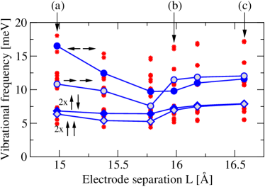
Figure 3: (Color online) Vibrational frequencies versus electrode displacement. The connected data series refer to the situation where only the two apex atoms are vibrating (resulting in the six vibrational modes indicated in the plot); circles symbolize the two longitudinal modes (CM and ABL) and diamonds the four (pair-wise degenerate) transversal modes. The red stars are the corresponding vibrational frequencies when also the pyramid bases are considered active. The three regimes are clearly identifiable: (a) concerted apex vibrations, (b) crossover where the stretch modes become degenerate, and (c) independent apex vibrations.

The evolution of the interaction between the apex atoms with distance is also revealed in the study of the vibrational modes. This is presented in Fig. 3, where the blue connected data points correspond to the 6 modes where only the apex atoms vibrate, and the red crosses to the 30 modes where also the pyramid bases vibrate. These modes follow different behavior with the electrode separation.

In the following we analyze the simplest case of just the two apex atoms. Generally, two longitudinal stretch modes (represented with connected circles in Fig. 3) line up the highest in energy. For an electrode distance larger than $L=16.5$ Å these correspond to the isolated (i.e., decoupled and hence degenerate) stretch modes of each apex atom, Fig. 3(c). As the electrodes are approached, the attractive apex-apex interaction leads to a slight displacement of the apex atoms away from the base of the pyramids. The consequence is a small weakening of the apex-atom coupling to the base which results in decreasing frequencies, i.e., to softening of the modes. Another consequence of the increasing interaction is the splitting of the degenerate modes into a symmetric (out–of–phase) and an antisymmetric (in–phase) mode. We will refer to these as the alternating bond length (ABL) modeFrederiksen:2004 and the center of mass (CM) mode, respectively. When the electrode separation reaches the region between $L=15.8$ Å and $L=16.0$ Å the frequencies drop significantly, Fig. 3(b). This points again at the chemical interaction crossover that we presented in the previous paragraph: now the interaction between the apex atoms becomes comparable with the interaction with the electrodes and hence weakens the stretch modes initially set by the interaction between the apex atom with the base of the pyramid. As the apex-apex interaction grows larger, the modes start to increase in frequency and further show an significant split, Fig. 3(a).

The behavior of the two stretch modes of Fig. 3 is easily understood with a simple one-dimensional elastic model of two masses, each coupled to infinite-mass system with a spring constant $k_{1}$, and interconnected by another spring constant $k_{2}$. The frequencies of the two stretch modes are then $\omega_{\textrm{CM}}=\sqrt{k_{1}/m}$ (in–phase) and $\omega_{\textrm{ABL}}=\sqrt{(k_{1}+2k_{2})/m}$ (out–of–phase), where $m$ is the mass of each atom. Note that in the tunneling regime the apex-apex interaction is attractive, cf. Fig. 2, which would correspond to a negative value of $k_{2}$. When the bond has been formed, $k_{2}$ can be represented as classical (positive) spring constant. This model essentially captures the evolution of the stretch modes. In particular, the sign change of $k_{2}$ at the chemical instability explains the mode crossing between $L=15.8$ Å and $L=16.0$ Å, Fig. 3(b), and why the CM mode has a higher frequency than the ABL mode in the tunneling case, and vice versa in the contact case.

The analysis of the modes with electrode distance thus permits us to recover the same range of distances with the chemical crossover as in the preceding section concerning the total energy and strain. This identification is also possible from the more realistic calculation that includes the vibration of the base atoms.

IV Elastic conductance

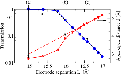
Figure 4: (Color online) Transmission $\tau$ (blue disks) and apex-apex distance $d$ (red crosses) versus electrode separation $L$. In the tunneling regime the transmission decays exponentially with separation as indicated with the dashed line (corresponding to a tunneling parameter $\Lambda=1.54~{}\textrm{\AA}^{-1}$). The point at (a) corresponds well with the contact region of transmission one and closest apex separation, (b) is near half transmission and the instability in apex separation, (c) is finally the tunneling regime, where the apex atoms are independent.

In this study we are interested in the low-bias regime. Hence the elastic conductance is determined via Landauer’s formula by the transmission at the Fermi energy $\varepsilon_{\textrm{F}}$. As expected for the gold contact, we find that the total transmission is essentially due to a single eigenchannel (for the geometries considered here the contribution from the secondary channel is at least three orders of magnitude smaller). Figure 4 plots the transmission $\tau$ and the apex-apex distance $d$ as a function of electrode separation $L$. In the tunneling regime the transmission is characterized by an exponential decay with separation. It is instructive to compare this with the transmission probability $T\propto\exp(-2\Lambda D)$ for a rectangular one-dimensional barrier, where $\Lambda=\sqrt{2m_{e}\Phi}/\hbar$ is a characteristic tunneling length, $\Phi$ the apparent barrier height, and $D$ the barrier width (valid for $\Lambda D\gg 1$). As shown in Fig. 4, an exponential fit to the calculated tunneling data leads to a tunneling parameter $\Lambda=1.54~{}\textrm{\AA}^{-1}$ which would correspond to an apparent barrier height of the order $\Phi\approx 9.1$ eV. Compared with measurements of the work function on perfectly flat Au surfaces (5.31–5.47 eV)Handbook:2007 this value is certainly high. On the other hand $\Phi$ is not very well determined from an exponential fit to data spanning only one decade. Another contribution to a relatively large barrier height could be geometric effects from the pyramidal shapes.

The deviation from the exponential tunneling behavior (visible around $L=16.0$ Å) is a clear indication of the crossover to contact. The contact regime is characterized by a constant transmission equal to unity since an atomic gold junction has effectively only one conduction channel. The value $\tau=1/2$ to define the crossover between contact and tunneling is somewhat arbitrary, however a detailed comparison with the previous section justifies this definition. Indeed, Fig. 4 also shows the behavior of the apex-atom distance $d$ with electrode separation, permitting us to make contact with the chemical crossover defined previously. Between $L=15.8$ Å and 16.0 Å we find that the apex-apex distance has changed by almost 0.7 Å. This shows that at these electrode distances, there is an instability that drive the formation of a covalent bond between apex atoms. This agrees with the conclusion from both total energy, strain and frequency calculations that the crossover takes place between 15.8 Å and 16.0 Å. From Fig. 4 we identify a transmission 1/2 associated with $L=15.9$ Å ($d=3.7$ Å) hence permitting us to identify the crossover from tunneling to contact with the chemical crossover.

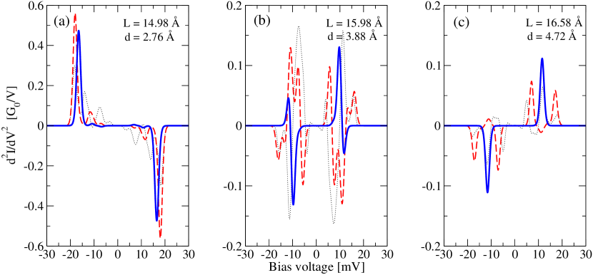
Figure 5: (Color online) Second derivative of the current versus bias voltage for three characteristic situations (a) contact, (b) crossover, and (c) tunneling. In each situation we consider different active vibrational regions: the two apex atoms only (thick blue line), the 10 pyramid atoms (thick dashed red curve), and both pyramids and first-layer atoms (dotted thin black curve). The signal broadening is due to temperature ($T=$ 4.2 K).

V Inelastic conductance

The behavior of the inelastic contributions to conductance is very different in the two studied regimes. In the tunneling regime the opening of the inelastic channel enhances the conductance of the system, while the creation of a vibrational excitation in a high conductance regime is a source of backscattering that decreases the conductance. Figure 5 shows the calculated change in conductance (second derivative of the current with respect to bias voltage $d^{2}I/dV^{2}$) for the contact, crossover and tunneling regions. These three typical cases—labeled (a), (b), and (c), respectively—are indicated in the previous Figs. 2–4 for easy reference. We investigate how the inelastic conductance change depends on how many atoms in the junction that are considered active: in Fig. 5 the thick blue line is the spectrum corresponding to only the two apex atoms vibrating, the dashed red curve to the 10 pyramid atoms vibrating, and the dotted black curve to the pyramids and first-layer atoms vibrating (42 atoms). In this way we follow the convergence of the calculations as the vibrational region is gradually enlarged. The essential data from these calculations are summarized in Tab. 1.

From the simplest case when only the two apex atoms are vibrating, we arrive at the conclusion that only the two longitudinal stretch modes contribute to the change in conductance, leading to the qualitative known result of increase of the conductance in tunneling regime and decrease in contact. The crossover case Fig. 5(b) presents a combination of an increase in conductance from the ABL mode and a decrease from the CM mode.

This behavior is a signature of the different processes of conduction. In the tunneling case, the tunneling process is determined by the more slowly-decaying components of the electron wave function of the surface. Because of the exponential tunneling probability dependence on distance a mode that modulates the tunneling gap is expected to contribute positively to the conductance.Lorente:2005 Indeed this is the case for the ABL mode. Furthermore, the CM mode that correspond to a fixed apex-apex distance cannot contribute positively, neither the transverse modes because none of them decrease the apex-apex distance from the equilibrium position during a vibration period. Instead, the CM mode is found to contribute negatively to the conductance, cf. Tab. 1. A simplified model presented in the next section will explain this observation.

In the contact case, the electronic structure responsible for the conduction process is largely concentrated upon the apex atom, hence the transport is being modified by the motion of basically only these atoms. Indeed both the ABL and CM modes lead to drops in the conductance as is evident from Fig. 5(a) and Tab. 1. The transverse modes give essentially no signal; this is similar to the findings for atomic gold wires where the transverse modes cannot couple because of symmetry.Frederiksen:2004 ; Frederiksen:2006

Figure 5 shows how the inelastic spectrum is modified if we increase the vibrational region by allowing more atoms to vibrate. In the tunneling and contact cases we see that the single main peak splits up into a number of peaks, indicating that the apex vibrations are actually coupled with the vibrations in the bulk. For the contact case the broadening of the signals is expected to be directly influenced by the phonon density of states of the bulk. As was first shown by Yanson,Yanson:1974 the spectroscopy of microcontacts at low temperatures—a technique nowadays referred to as point contact spectroscopy—reveals a signal in $d^{2}I/dV^{2}$ which is a direct measurement of the Eliashberg function $\alpha^{2}F$, i.e., roughly speaking the product of the squared electron-phonon coupling matrix element $\alpha$ and the phonon density of states $F$, averaged over the Fermi sphere.Jansen:1980 In the case of microcontacts the measured signal is predominantly due to the transverse modes. This is in contrast to our case of the atomic point contact, where we only find signals from the longitudinal modes. However, from Fig. 5(a) we notice a signal broadening by increasing the vibrational region, pointing towards the vibrational coupling to the bulk modes.

In the crossover region between tunneling and contact, Fig. 5(b) shows a dramatic change depending on the size of the vibrational region. Different modes give positive or negative contributions in the conductance, but in such a way that they lead to an overall absence of (or relatively small) variation in the conductance, cf. Tab. 1.

Comparing the total change in conductance $\Delta G=G(V\gg\hbar\omega_{\lambda})-G(V=0)$ induced by all modes (for the tunneling, crossover, and contact situations), we find that the calculations with different vibrational regions give almost the same results. As found in Tab. 1, we thus conclude that to a first approximation we can describe $\Delta G\approx\delta G_{\textrm{ABL}}+\delta G_{\textrm{CM}}$, i.e., the overall conductance change can be estimated with the minimal vibrational region (the two apex atoms). This simple approach does however not accurately describe details of the $d^{2}I/dV^{2}$ spectrum.

L	d		$\tau$		$\omega_{\textrm{ABL}}$	$\delta G_{\textrm{ABL}}/\mathrm{G}_{0}\tau$		$\omega_{\textrm{CM}}$	$\delta G_{\textrm{CM}}/\mathrm{G}_{0}\tau$		$\Delta G/G$		$\Delta G/G$		$\Delta G/G$
[Å]	[Å]		-		[meV]	[%]		[meV]	[%]		[%]		[%]		[%]
14.98	2.76		0.988		16.52	-0.104		10.83	-0.002		-0.105		-0.146		-0.151
15.38	2.88		0.978		12.46	-0.145		9.81	-0.005		-0.149		-0.206		—
15.78	3.23		0.857		7.57	-0.223		9.73	-0.014		-0.235		-0.340		—
15.98	3.88		0.395		9.80	0.077		11.47	-0.035		0.045		-0.006		-0.032
16.18	4.22		0.208		11.00	0.224		11.86	-0.045		0.181		0.193		—
16.58	4.72		0.063		11.60	0.430		12.04	-0.053		0.377		0.395		0.332

Table 1: Characteristic data for the six structures representing the evolution of the junction from tunneling to contact regimes. The columns describe the electrode separation $L$, apex-apex distance $d$, transmission $\tau$, vibrational energies $\hbar\omega_{\lambda}$ and mode-specific conductance changes $\delta G_{\lambda}$ (for the ABL and CM modes), and the total conductance change $\Delta G/G$ from all modes (calculated for three different sizes of the vibrational region).

VI Discussion

The effect of the tunneling to contact crossover has important implications in the inelastic conductance since in the first case the inelastic effects trend to increase and in the second case to diminish the electron conduction. From the results of the previous section, we have seen that this crossover roughly takes place at the same range of distances as in the elastic conductance case. By looking at the transmission in the elastic conductance case, we conclude that when the transmission is $\tau=1/2$ we should also be near the crossover between tunneling to contact in the inelastic case one. This finding is similar to the crossover found for the single-state impurity model analyzed in Ref. [Paulsson:2005, ]. However, in the present case, the system is not obviously modeled with a single-state impurity. Instead we can easily reproduce the same kind of analysis for a slightly more sophisticated model, where two impurities are connected to reservoirs and interacts via a hopping term between them. Under symmetric conditions this system is described by

$$\mathbf{H}=\left[\begin{array}[]{cc}\varepsilon_{0}&t\\ t&\varepsilon_{0}\end{array}\right],\quad\mathbf{\Gamma}_{L}=\left[\begin{array}[]{cc}\gamma&0\\ 0&0\end{array}\right],\quad\mathbf{\Gamma}_{R}=\left[\begin{array}[]{cc}0&0\\ 0&\gamma\end{array}\right],$$ (11)

where the Hamiltonian $\mathbf{H}$ includes on-site energies $\varepsilon_{0}$ and a hopping matrix element $t$. The level broadening functions $\mathbf{\Gamma}_{\alpha}$ describes the coupling of the sites to the contacts $\alpha=L,R$ with strength $\gamma$ (which in the wide band approximation are considered energy independent). The corresponding retarded Green’s function is

$$\mathbf{G} = [\varepsilon_{\textrm{F}}\mathbf{1}-\mathbf{H}+i(\mathbf{\Gamma}_{L}+\mathbf{\Gamma}_{R})/2]^{-1}$$ (14)

$$= \frac{2}{(2\Delta\varepsilon+i\gamma)^{2}-4t^{2}}\left[\begin{array}[]{cc}2\Delta\varepsilon+i\gamma&2t\\ 2t&2\Delta\varepsilon+i\gamma\end{array}\right],\qquad$$

where in our case $\Delta\varepsilon=\varepsilon_{\textrm{F}}-\varepsilon_{0}\ll\gamma$ holds since the level positions would be close to the Fermi energy $\varepsilon_{\textrm{F}}$ (the on-resonance case). The transmission becomes

$$\tau=\frac{16t^{2}\gamma^{2}}{\left(4t^{2}+\gamma^{2}\right)^{2}}+\mathcal{O}(\Delta\varepsilon^{2}),$$ (15)

where perfect transmission $\tau=1$ is obtained for $t=\gamma/2$.

Inspired by our electron-phonon coupling matrices obtained from the full DFT calculations, we assign the following forms to the longitudinal ABL and CM mode couplings

$$\mathbf{M}_{\textrm{ABL}}=\left[\begin{array}[]{cc}m_{1}&m_{2}\\ m_{2}&m_{1}\end{array}\right],\quad\mathbf{M}_{\textrm{CM}}=\left[\begin{array}[]{cc}m_{3}&0\\ 0&-m_{3}\end{array}\right].$$ (20)

The ABL mode is symmetric and generally described by two coupling strengths: $m_{1}$ represents an on-site modification via a change in the electrode coupling, whereas $m_{2}$ is a modulation of the hopping between the apexes. Correspondingly, the CM mode which is asymmetric bears an asymmetric on-site modulation $m_{3}$ and no hopping modulation (fixed apex-apex distance). With these expressions we can simply evaluate Eq. (4) to find the following inelastic conductance changes

$$\frac{\delta G_{\textrm{ABL}}}{\mathrm{G}_{0}\tau} = \frac{\left(16t^{4}-24\gamma^{2}t^{2}+\gamma^{4}\right)}{\left(4t^{2}+\gamma^{2}\right)^{2}}$$ (21)

$$\times\left(\frac{{m_{2}}^{2}}{t^{2}}+\frac{16m_{1}m_{2}\Delta\varepsilon}{4t^{3}+t{\gamma}^{2}}+\mathcal{O}(\Delta\varepsilon^{2})\right),$$

$$\frac{\delta G_{\textrm{CM}}}{\mathrm{G}_{0}\tau} = -\frac{16m_{3}^{2}\gamma^{2}}{\left(4t^{2}+\gamma^{2}\right)^{2}}+\mathcal{O}(\Delta\varepsilon^{2}),$$ (22)

We first discuss the conclusions to be drawn about the ABL mode. Notice that $\delta G_{\textrm{ABL}}$ is only weakly dependent on the the on-site coupling element $m_{1}$ and vanishes on resonance ($\Delta\varepsilon=0$). In the tunneling limit ($t\rightarrow 0$) we find that

$$\lim_{t\rightarrow 0}\frac{\delta G_{\textrm{ABL}}}{\textrm{G}_{0}}=\frac{16m_{2}^{2}}{{\gamma}^{2}}+\mathcal{O}(\Delta\varepsilon^{2}),$$ (23)

i.e., the ABL mode gives a positive contribution to the conductance proportional to the square of coupling strength $m_{2}$. In the contact limit ($\tau\rightarrow 1$) we find

$$\lim_{\tau\rightarrow 1}\frac{\delta G_{\textrm{ABL}}}{\textrm{G}_{0}}=-\frac{4m_{2}^{2}}{{\gamma}^{2}}-\frac{16m_{1}m_{2}\Delta\varepsilon}{{\gamma}^{3}}+\mathcal{O}(\Delta\varepsilon^{2}),$$ (24)

i.e., the ABL mode gives here a negative contribution. The exact crossover between an increase and a decrease is determined by solving $\delta G_{\textrm{ABL}}=0$, which indeed yields $\tau=1/2$ as is the case for the single-site case.Paulsson:2005

Next, we see from Eq. (22) that the conductance change $\delta G_{\textrm{CM}}$ from the CM mode is always negative (i.e., the CM mode backscatters even in the tunneling regime).

These results thus permit to rationalize the crossover from tunneling to contact for the inelastic conductance—as found numerically in Sec. V—as taking place around a transmission of $\tau=1/2$.

VII Summary and conclusions

The evolution of the inelastic signals from the tunneling to contact regimes has been studied through DFT calculations. We have compared our results with the crossover between bonding and rupture of the atomic junction by studying the geometric and electronic structures of the junction, together with the strength of the atomic bonds and the associated vibrational frequencies. This permitted us to find a typical transition distance between electrodes where a small change leads to a large readjustment of the apex-apex atom distance, as well as a change of the strength of interactions as revealed by the total energy, the strain and the frequencies of the system’s modes.

The conductance has been calculated by first evaluating the transmission of electrons through the system, and second by calculating the conductance change due to the excitation of vibrations. As found in previous studiesPaulsson:2005 the change in conductance due to inelastic effects permits to characterize the crossover from tunneling to contact. The most notorious effect being a decrease of conductance in the contact regime to an increase in the tunneling one when the bias voltage exceeds the vibrational thresholds. Our DFT-based calculations show that the effect of vibrational modes in the $d^{2}I/dV^{2}$ spectra is rather complex, in particular when modes localized in the contact region are permitted to extend into the electrodes. As an example, we find that certain modes can give rise to decreases in conductance when in the tunneling regime, opposite to the above mentioned result. Whereas details in the inelastic spectrum depends sensitively on the size of the vibrational region, we find that the magnitude of the overall change in conductance can actually be reasonably described with just the minimal case where only the apex atoms vibrate. This means that while the modes are rather delocalized the region of inelastic scattering is localized around the apex atoms.

By comparing our results with a simplified model, we conclude that in this single eigenchannel problem the tunneling to contact crossover takes place exactly at $\tau=1/2$, in agreement with the findings for the elastic conduction process and the chemical crossover. Hence, we can trace back the origin of the conduction process, both in the presence and absence of vibrational excitation, to the same type of underlying electron structure that determine the electrode’s chemical interaction and the electron conductance.Hofer:2003

- (1) N. Agraït, A. L. Yeyati, and J. M. van Ruitenbeek, Phys. Rep. 377, 81 (2003).
- (2) R. C. Stipe, M. A. Rezaei, and W. Ho, Science 280, 1732 (1998).
- (3) J. I. Pascual, Eur. Phys. J. D 35, 327 (2005).
- (4) T. Komeda, Prog. Surf. Sci. 78, 41 (2005).
- (5) N. Agraït, C. Untiedt, G. Rubio-Bollinger, and S. Vieira, Phys. Rev. Lett. 88, 216803 (2002); Chem. Phys. 281, 231 (2002).
- (6) T. Frederiksen, M. Brandbyge, N. Lorente, and A.-P. Jauho, Phys. Rev. Lett. 93, 256601 (2004).
- (7) R. H. M. Smit, Y. Noat, C. Untiedt, N. D. Lang, M. C. van Hemert, and J.M. van Ruitenbeek, Nature 419, 906 (2002).
- (8) M. Galperin, M. A. Ratner, and A. Nitzan, Jour. Chem. Phys. 121, 11965 (2004).
- (9) M. Paulsson, T. Frederiksen, and M. Brandbyge, Phys. Rev. B. 72, 201101(R) (2005).
- (10) J. K. Viljas, J. C. Cuevas, F. Pauly, and M. Hafner, Phys. Rev. B 72, 245415 (2005).
- (11) L. de la Vega, A. Martin-Rodero, N. Agraït, and A. L. Yeyati, Phys. Rev. B 73, 075428 (2006).
- (12) J. R. Hahn, H. J. Lee, and W. Ho, Phys. Rev. Lett. 85, 1914 (2000).
- (13) B. N. J. Persson and A. Baratoff, Phys. Rev. Lett. 59, 339 (1987).
- (14) N. Lorente, Appl. Phys. A. 78, 799 (2004).
- (15) C. Untiedt, M. J. Caturla, M. R. Calvo, J. J. Palacios, R. C. Segers, and J. M. van Ruitenbeek, cond-mat/0611122.
- (16) L. Limot, J. Kröger, R. Berndt, A. Garcia-Lekue, W. A. Hofer, Phys. Rev. Lett. 94, 126102 (2005).
- (17) J. M. Soler, E. Artacho, J. D. Gale, A. Garcia, J. Junquera, P. Ordejon, and D. Sanchez-Portal, J. Phys.: Cond. Mat. 14, 2745 (2002).
- (18) M. Brandbyge, J. L. Mozos, P. Ordejon, J. Taylor, and K. Stokbro, Phys. Rev. B 65 165401 (2002).
- (19) T. Frederiksen, M. Paulsson, M. Brandbyge, and A.-P. Jauho, accepted in PRB, cond-mat/0611562.
- (20) N. Lorente, R. Rurali, and H. Tang, J. Phys.: Cond. Mat. 17, S1049 (2005).
- (21) CRC Handbook of chemistry and physics, 87th ed. (2007).
- (22) I. K. Yanson, Zh. Eksp. Teor. Fiz. 66, 1035 (1974) [Sov. Phys.-JETP 39, 506 (1974)].
- (23) A. G. M. Jansen, A. P. van Gelder, P. Wyder, J. Phys. C: Solid St. Phys., 13, 6073-118 (1980).
- (24) W. A. Hofer and A. J. Fisher, Phys. Rev. Lett. 91, 036803 (2003); Phys. Rev. Lett. 96, 069702 (2006).