Bright solitons and soliton trains in a fermion-fermion mixture

Abstract

We use a time-dependent dynamical mean-field-hydrodynamic model to predict and study bright solitons in a degenerate fermion-fermion mixture in a quasi-one-dimensional cigar-shaped geometry using variational and numerical methods. Due to a strong Pauli-blocking repulsion among identical spin-polarized fermions at short distances there cannot be bright solitons for repulsive interspecies fermion-fermion interactions. However, stable bright solitons can be formed for a sufficiently attractive interspecies interaction. We perform a numerical stability analysis of these solitons and also demonstrate the formation of soliton trains. These fermionic solitons can be formed and studied in laboratory with present technology.

Recent observations exp1 ; exp2 ; exp3 ; exp4 and associated experimental exp5 ; exp5x ; exp6 and theoretical yyy1 ; yyy ; capu ; capu1 ; ska studies of a degenerate Fermi gas (DFG) by sympathetic cooling in the presence of a second boson or fermion component suggest the possibility of soliton formation. Apart from the observation of a DFG in the following degenerate boson-fermion mixtures (DBFM) ^6,7Li exp3 , ²³Na-⁶Li exp4 and ⁸⁷Rb-⁴⁰K exp5 ; exp5x , there have been studies of degenerate spin-polarized fermion-fermion mixtures (DFFM) ⁴⁰K-⁴⁰K exp1 and ⁶Li-⁶Li exp2 .

Bright solitons in a Bose-Einstein condensate (BEC) are formed due to an attractive nonlinear atomic interaction exdks . As the interaction in a pure DFG at short distances is repulsive due to strong Pauli blocking, there cannot be bright solitons in a DFG. However, it has been demonstrated fbs1 ; fbs2 that bright solitons can be formed in a DBFM in the presence of a sufficiently strong boson-fermion attraction which can overcome the Pauli repulsion among identical fermions.

We demonstrate the formation of stable fermionic bright solitons in a DFFM for a sufficiently attractive interspecies fermion-fermion interaction. In a DFFM, the coupled system can lower its energy by forming high density regions, the bright solitons, when the attraction between the two types of fermions is large enough to overcome the Pauli repulsion among identical fermions. We use a coupled time-dependent mean-field-hydrodynamic model for a DFFM and consider the formation of axially-free localized bright solitons in a quasi-one-dimensional cigar-shaped geometry using numerical and variational solutions. The present model is inspired by the success of a similar model suggested recently by the present author in the investigation of collapse ska and bright fbs2 and dark fds solitons in a DBFM. We study the condition of modulational instability of a constant-amplitude solution in this model and demonstrate the possibility of the formation of bright solitons. We also present a numerical stability analysis of these robust bright solitons and consider the formation of a soliton train in a DFFM by a large sudden jump in the interspecies fermion-fermion scattering length near a Feshbach resonance, experimentally observed in both ⁶Li-⁶Li and ⁴⁰K-⁴⁰K fesh .

We use a simplified mean-field-hydrodynamic Lagrangian for a DFG used successfully to study a DBFM ska ; fbs2 ; fds . The virtue of the mean-field model over a microscopic description is its simplicity and predictive power. To develop a set of time-dependent mean-field-hydrodynamic equations for the interacting DFFM, we use the following Lagrangian density ska ; fbs2

$${\cal L} =g_{12}n_{1}n_{2}+\sum_{j=1}^{2}\frac{i}{2}\hbar\left[\psi_{j}\frac{\partial{\psi_{j}}^{*}}{\partial t}-{\psi_{j}}^{*}\frac{\partial\psi_{j}}{\partial t}\right]$$ (1)

$$+ \sum_{j=1}^{2}\left(\frac{\hbar^{2}|\nabla_{\bf r}\psi_{j}|^{2}}{6m_{j}}+V_{j}({\bf r})n_{j}+\frac{3}{5}A_{j}n_{j}^{5/3}\right),$$

where $j=1,2$ represents the two components, $\psi_{j}$ the complex probability amplitude, $n_{j}=|\psi_{j}|^{2}$ the real probability density, ^∗ denotes complex conjugate, $m_{j}$ the mass, $A_{j}=\hbar^{2}(6\pi^{2})^{2/3}\-\-/(2m_{i}),$ the interspecies coupling $g_{12}=2\pi\hbar^{2}a_{12}/m_{R}$ with $m_{R}=m_{1}m_{2}/(m_{1}+m_{2})$ the reduced mass, and $a_{12}$ the interspecies fermion-fermion scattering length. The number of fermionic atoms $N_{j}$ is given by $\int d{\bf r}n_{j}({\bf r})=N_{j}$. The trap potential with axial symmetry is $V_{j}({\bf r})=\frac{1}{2}m_{j}\omega^{2}(\rho^{2}+\nu^{2}z^{2})$ where $\omega$ and $\nu\omega$ are the angular frequencies in the radial ($\rho$) and axial ($z$) directions with $\nu$ the anisotropy. The interaction between identical intra-species fermions in spin-polarized state is highly suppressed due to Pauli blocking terms $3A_{j}n_{j}^{5/3}/5$ and has been neglected in Eq. (1). The kinetic energy terms $\hbar^{2}|\nabla_{\bf r}\psi_{j}|^{2}/(6m_{j})$ in Eq. (1) contribute little to this problem compared to the dominating Pauli-blocking terms. However, its inclusion leads to an analytic solution for the probability density everywhere fbs2 .

With the Lagrangian density (1), the following Euler-Lagrange equations can be derived in a straight-forward fashion ska ; fbs2 :

$$\biggr{[}i\hbar\frac{\partial}{\partial t}+\frac{\hbar^{2}\nabla_{\bf r}^{2}}{6m_{{j}}}-V_{{j}}-A_{j}n_{j}^{2/3}-g_{{12}}n_{k}\biggr{]}\psi_{j}=0,$$ (2)

where $j\neq k=1,2$. This is essentially a time-dependent version of a similar time-independent model used recently for fermions capu . For large $n_{j}$, both lead to the Thomas-Fermi result $n_{j}=[(\mu_{j}-V_{j})/A_{j}]^{3/2}$ capu ; ska with $\mu_{j}$ the chemical potential. As the bright solitons of this rapid note are stationary states, they could be obtained by the time-independent approach used in Ref. capu . The stationary approach of Ref. capu has passed rigorous tests of comparison of the hydrodynamic-mean-field spectra of localized fermions with the spectra calculated in the collisionless regime within the random-phase approximation (RPA). The results of mixing-demixing and collapse of the hydrodynamic approach are in agreement with the RPA analysis capu1 . The detailed behavior of collective excitation of trapped fermions has also been found to agree with that obtained by an RPA analysis capu . For a description of stationary solitons (e.g., of Fig. 1) we could have used the well-established formulation of Ref. capu to obtain identical results, as the present time-dependent dynamical description and the time-independent approach of capu yield identical results for stationary states. However, we shall be using the present time-dependent dynamical formulation to study the nonequilibrium generation soliton trains, in addition.

We reduce three-dimensional Eqs. (2) to a minimal quasi-one-dimensional form in a cigar-shaped geometry with $\nu<<1$, where the radial motion is frozen in the ground state of the harmonic trap and the dynamics is carried by the axial motion. For radially-bound and axially-free solitons we eventually set $\nu=0$. Following Ref. fbs2 this reduction can be done in a straight-forward fashion and we quote the final results here:

$$\biggr{[}i\frac{\partial}{\partial\tau}+\frac{\partial^{2}}{\partial y^{2}}-N_{jj}\left|{{\phi}_{j}}\right|^{4/3}+N_{jk}\left|{{\phi}_{k}}\right|^{2}\biggr{]}{\phi}_{{j}}({y},\tau)=0,$$ (3)

where $\phi_{j},j\neq k=1,2$ represents the two solitons, $\tau=t\omega/2$, $y=z/l$, $N_{jj}=9(6\pi N_{j})^{2/3}/5,$ $N_{jk}=12|a_{12}|N_{k}/l,$ $l=\sqrt{\hbar/(\omega m)}$, with $m=3m_{1}=3m_{2}$. Here we employ equal-mass fermions, a negative $a_{12}$ corresponding to attraction, and normalization $\int_{-\infty}^{\infty}|\phi_{j}(y,\tau)|^{2}dy=1.$ In Eqs. (3) a sufficiently strong attractive fermion-fermion coupling $N_{jk}|\phi_{k}|^{2}(j\neq k)$ can overcome the Pauli repulsion $N_{jj}|\phi_{j}|^{4/3}$ and form bright solitons.

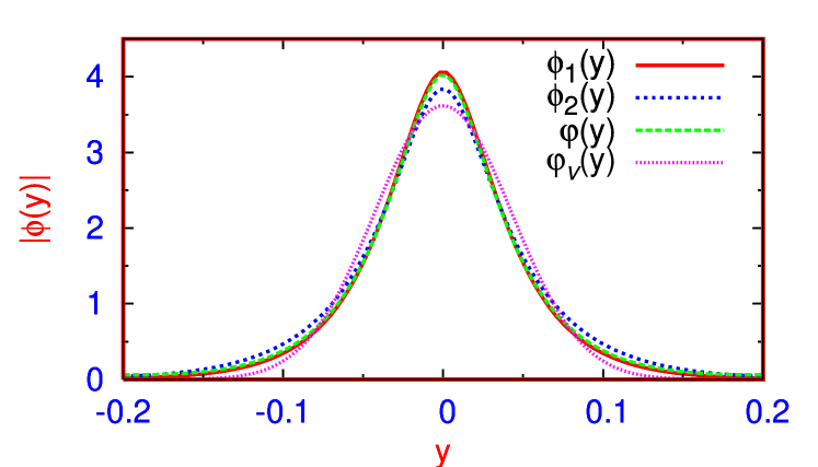
Figure 1: (Color online) The solitons $|\phi_{j}(y)|$ of Eq. (3) vs. $y$ (in dimensionless units) for $N_{1}=44$, $N_{2}=56$, $a_{12}=-0.3$ nm, while $N_{11}\approx 159$, $N_{12}\approx 203$, $N_{21}\approx 160$, and $N_{22}\approx 187$. The variational $(\varphi_{v})$ and numerical $(\varphi)$ solutions of Eq. (4) for $N_{1}=N_{2}=50$ are also shown.

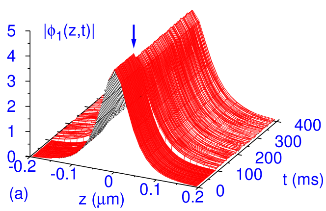
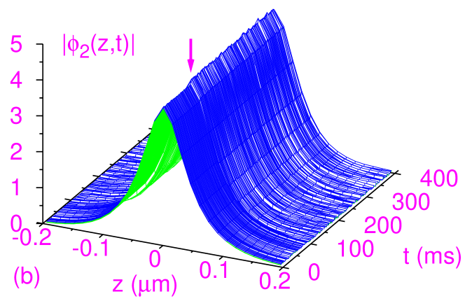
Figure 2: (Color online) The propagation of fermionic solitons (a) $|\phi_{1}(z,t)|$ and (b) $|\phi_{2}(z,t)|$ of Fig. 1 vs. $z$ and $t$. At $t=100$ ms (marked by arrows) the bright solitons are set into small breathing oscillation by suddenly changing $N_{1}=44$ and $N_{2}=56$ to $N_{2}=44$, $N_{1}=56$.

Now we perform a stability analysis of constant-amplitude solutions of Eqs. (3) and study the possibility of generation of solitons in the symmetric case: $N_{1}=N_{2}$, when $\phi_{1}=\phi_{2}\equiv\varphi$ and these equations reduce to

$$\biggr{[}i\frac{\partial}{\partial\tau}+\frac{\partial^{2}}{\partial y^{2}}-\beta\left|{\varphi}\right|^{4/3}+\gamma\left|{{\varphi}}\right|^{2}\biggr{]}{\varphi}({y},\tau)=0,$$ (4)

where $\beta=N_{11}=N_{22}$ and $\gamma=N_{12}=N_{21}$. We consider the constant-amplitude solution 1 $\varphi_{0}=A_{0}\exp(i\delta)\equiv A_{0}\exp[i(\gamma A_{0}^{2}\tau-\beta A_{0}^{4/3}\tau)]$ of Eq. (4) under small perturbation: $\varphi=(A_{0}+A)\exp(i\delta)$, where $A=A(y,\tau)$ and $A_{0}$ the amplitude. Substituting this perturbed solution in Eq. (4), and for small perturbations retaining only the linear terms in $A$ we get

$$i\frac{\partial A}{\partial\tau}+\frac{\partial^{2}A}{\partial y^{2}}-\frac{2}{3}\beta A_{0}^{4/3}(A+A^{*})+\gamma A_{0}^{2}(A+A^{*})=0.$$ (5)

We consider the plane-wave perturbation $A(y,\tau)=A_{1}\-\cos(K\tau-\Omega y)+iA_{2}\sin(K\tau-\Omega y)$ in Eq. (5). Then separating the real and imaginary terms and eliminating $A_{1}$ and $A_{2}$ we obtain the dispersion relation $K=\pm\Omega[\Omega^{2}$ $-(2\gamma A_{0}^{2}-4\beta A_{0}^{4/3}/3)]^{1/2}.$ For stability of the plane-wave perturbation, $K$ has to be real. This happens for $2\gamma A_{0}^{2}<4\beta A_{0}^{4/3}/3$ or $\gamma A_{0}^{2/3}<2\beta/3$. However, $K$ can become imaginary for $\gamma A_{0}^{2/3}>2\beta/3$ and the plane-wave perturbations can grow exponentially with time $\tau$. This is the domain of modulational instability of a constant-intensity solution, signalling a tendency of spatially localized bright solitons to appear. We also performed this analysis in the case of non-symmetric coupled equations (3) and quote the result here. The condition for instability is $N_{12}N_{21}A_{10}^{2/3}A_{20}^{2/3}>4N_{11}N_{22}/9$ shuk , where $A_{10}$ and $A_{20}$ are the amplitudes of the two solutions.

Next we present a variational analysis of Eq. (4) based on the normalized Gaussian trial wave function and $\varphi_{v}(y,\tau)$ $=\sqrt{1/[a(\tau)\sqrt{\pi}]}\exp[-y^{2}/\{2a^{2}(\tau)\}+ib(\tau)y^{2}/2]$, where $a$ is the width and $b$ the chirp. The Lagrangian density for Eq. (4) is the one-term version of Eq. (1), which is evaluated with this trial function and the effective Lagrangian $L=\int_{-\infty}^{\infty}{\cal L}(\varphi_{v})dy$ becomes

$$L=\frac{a^{2}}{4}\biggr{(}\dot{b}+\frac{2}{a^{4}}+2b^{2}-\frac{\sqrt{2}}{\sqrt{\pi}}\frac{\gamma}{a^{3}}+\frac{12\sqrt{3}}{5\sqrt{5}}\frac{\beta}{\pi^{1/3}a^{8/3}}\biggr{)}.$$ (6)

The variational Euler-Lagrangian equations for $a$ and $b$ can then be written and solved in a standard fashion and to yield the differential equation for the width: $d^{2}a/d\tau^{2}=[4-a\gamma\sqrt{2/\pi}+a^{4/3}(8\beta\sqrt{3})/(5\pi^{1/3}\sqrt{5})]/a^{3}$. The variational result for width $a$ follows by setting the right hand side of this equation to zero, from which the variational profile for the soliton can be obtained and .

We solve Eqs. (3) for bright solitons numerically using a time-iteration method based on the Crank-Nicholson discretization scheme elaborated in Ref. sk1 using time step $0.0002$ and space step $0.015$. We perform a time evolution of Eqs. (3) introducing an harmonic oscillator potential $y^{2}$ and setting the nonlinear terms to zero, and starting with the eigenfunction of the linear harmonic oscillator problem. The extra harmonic oscillator potential, which will be set equal to zero in the end, only aids in starting the time evolution with an exact analytic form. During the time evolution the nonlinear terms are switched on and the harmonic oscillator potential is switched off slowly and the time evolution continued to obtain the final converged solutions.

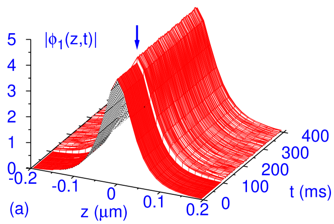
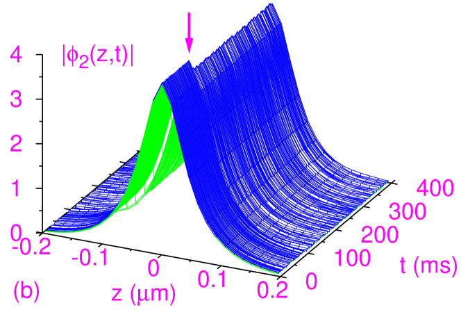
Figure 3: (Color online) The propagation of fermionic solitons (a) $|\phi_{1}(z,t)|$ and (b) $|\phi_{2}(z,t)|$ vs. $z$ and $t$. At $t=100$ ms (marked by arrows) the same initial solitons of Figs. 1 are set into small breathing oscillation by suddenly changing $\phi_{1}\to 1.1\phi_{1}$ and $\phi_{2}\to 0.9\phi_{2}$.

In our numerical study we take $l=1$ $\mu$m and consider a DFFM consisting of two electronic states of ⁴⁰K atoms. This corresponds to a radial trap of frequency $\omega\approx 2\pi\times 83$ Hz. Consequently, the unit of time is $2/\omega\approx 4$ ms.

First we solve coupled Eqs. (3) with $N_{1}=44,N_{2}=56$, and $a_{12}=-0.3$ nm. The soliton profile in this case is shown in Fig. 1, where we also plot the variational and numerical solutions of Eq. (4) for $N_{1}=N_{2}=50$. In this case in Eq. (4) $\beta\approx 173$ and $\gamma\approx 181.6$ leading to a variational width $a\approx 0.043$ and a variational soliton profile $\varphi_{v}\approx 3.62\exp(-270y^{2})$. The variational result agrees well with the numerical solutions.

At this stage it is pertinent to see if Friedel oscillations fri of density of the localized fermions are small so that the effective description of the solitons is valid. An one-dimensional degenerate Fermi gas of $N$ atoms filled up to Fermi sea has a spatial extension $2L_{F}=l\sqrt{2N-1},$ where $l$ is a measure of confinement gle . In the presence of an harmonic trap, $l$ is the harmonic trap length and is smaller than the spatial extension of the confined fermions. In the case of the soliton of Fig. 2, a typical measure of $l$ could be 0.05 $\mu$m so that for about 50 fermions considered here $2L_{F}=0.5$ $\mu$m. The Fermi momentum of an one-dimensional Fermi gas is $k_{F}=\pi N/(2L_{F})$ gle . The spatial wave-length of Friedel oscillation is gle $\lambda=\pi/k_{F}=2L_{F}/N\approx 0.01$ $\mu$m, much smaller than the soliton width of 0.1 $\mu$m. This qualitative analysis resulting in small Friedel oscillation supports the effective description used this rapid note for a DFFM.

To test the robustness of these solitons we inflicted different perturbations on them and studied the resultant dynamics numerically. First, after the formation of the solitons we suddenly changed the fermion numbers from $N_{1}=44$ and $N_{2}=56$ to $N_{1}=56,N_{2}=44$ at time $t=100$ ms. This corresponds to a sudden change of nonlinearities from $N_{11}\approx 159$, $N_{12}\approx 203$, $N_{21}\approx 160$, and $N_{22}\approx 187$ to $N_{11}\approx 187$, $N_{12}\approx 160$, $N_{21}\approx 203$, and $N_{22}\approx 159$. The resultant dynamics is shown in Figs. 2 (a) and (b). Due to the sudden change in nonlinearities the fermionic bright solitons are set into stable non-periodic small-amplitude breathing oscillation. Next on the same initial solitons of Figs. 2, at $t=100$ ms, we suddenly inflict the perturbation $\phi_{1}\to 1.1\phi_{1}$ and $\phi_{2}\to 0.9\phi_{2}$ and follow numerically the time evolution. The result of simulation is shown in Figs. 3 (a) and (b). We find that the solitons again continue non-periodic breathing oscillation and stabilize at large times. We also gave a small displacement between the centers of these solitons. We find that after oscillation and dissipation the solitons again come back to the stable configuration.

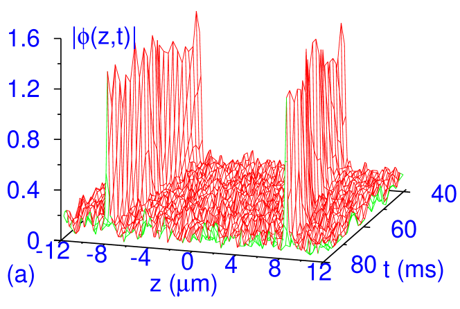
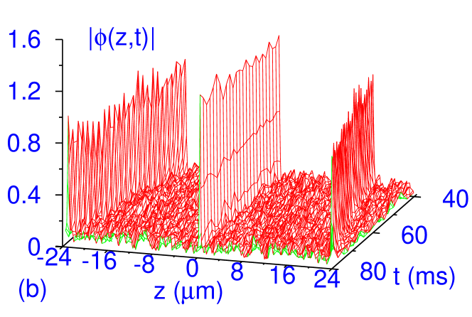
Figure 4: (Color online) Soliton trains of two and three solitons formed upon removing the harmonic trap $y^{2}$ and jumping the nonlinearities at $t=0$ from $N_{jj}\approx 173,N_{jk}\approx 145,k\neq j=1,2$ to (a) $N_{jj}\approx 173,N_{jk}\approx 273,$ and to (b) $N_{jj}\approx 173,N_{jk}\approx 309,$, respectively.

During the time evolution of Eqs. (3) if the nonlinearities are changed by a small amount or changed slowly, usually one gets a single stable soliton when the final nonlinearities are appropriate. However, if the nonlinearities are jumped suddenly by a large amount, a soliton train can be obtained as in the experiment with BEC exdks . To illustrate this we consider the solution of Eqs. (3) with nonlinearities $N_{jj}\approx 173$ and $N_{jk}\approx 145,j\neq k=1,2$ and harmonic oscillator trap $y^{2}$. After the formation of the solitons we suddenly jump the off-diagonal nonlinearities to $N_{jk}\approx 273$ and also switch off the harmonic trap at time $t=0$. Then after some initial noise and dissipation the time evolution of Eqs. (3) generates two slowly receding bright solitons of each component as shown in Fig. 4 (a). More solitons can be generated when the jump in the nonlinearities is larger. In Fig. 4 (b) we show the generation of three slowly receding solitons of each component upon a sudden jump of the off-diagonal nonlinearities to $N_{jk}\approx 309$ from the same initial state as in Fig. 4 (a). The formation of soliton trains from a stable initial state is due to modulational instability 1 . The sudden jump in the off-diagonal nonlinearities could be effected by a jump in the interspecies scattering length $a_{12}$ obtained by manipulating a background magnetic field near a fermion-fermion Feshbach resonance fesh .

In conclusion, we use a coupled mean-field-hydrodynamic model for a DFFM to study the formation of bright solitons and soliton trains in a quasi-one-dimensional geometry by numerical and variational methods. We find that an attractive interspecies interaction can overcome the Pauli blocking repulsion and form fermionic bright solitons in a DFFM. The stability of the present solitons is demonstrated numerically through their sustained breathing oscillation initiated by a sudden small perturbation. We also illustrate the creation of soliton trains upon a sudden large jump in off-diagonal nonlinearities. Bright solitons and soliton trains have been created experimentally in attractive BECs in the presence of a radial trap only without any axial trap exdks . In view of this, fermionic bright solitons and trains can be created in laboratory in a DFFM in a quasi-one-dimensional configuration. Here we used a set of mean-field equations for the DFFM. A proper treatment of a DFG or DFFM should be done using a fully antisymmetrized many-body Slater determinant wave function yyy1 ; fbs1 as in the case of scattering involving many electrons ps . However, in view of the success of a fermionic mean-field-hydrodynamic model in studies of collapse ska , bright fbs2 and dark solitons fds in a DBFM, and of mixing-demixing md and black solitons lpl in a DFFM, we do not believe that the present study on bright solitons in a DFFM to be so peculiar as to have no general validity.

The work is supported in part by the CNPq and FAPESP of Brazil.

References

- (1) B. DeMarco, D. S. Jin, Science 285 (1999) 1703.
- (2) K. M. O’Hara et al., Science 298 (2002) 2179.
- (3) F. Schreck et al., Phys. Rev. Lett. 87 (2001) 080403; A. G. Truscott et al., Science 291 (2001) 2570.
- (4) Z. Hadzibabic et al., Phys. Rev. Lett. 88 (2002) 160401.
- (5) G. Modugno et al., Science 297 (2002) 2240; C. Ospelkaus et al., Phys. Rev. Lett. 96 (2006) 020401.
- (6) G. Roati et al., Phys. Rev. Lett. 89 (2002) 150403.
- (7) K. E. Strecker, G. B. Partridge, R. G. Hulet, Phys. Rev. Lett. 91 (2003) 080406; Z. Hadzibabic et al., Phys. Rev. Lett. 91 (2003) 160401.
- (8) K. Molmer, Phys. Rev. Lett. 80 (1998) 1804.
- (9) R. Roth, Phys. Rev. A 66 (2002) 013614; T. Miyakawa, T. Suzuki, H. Yabu, Phys. Rev. A 64 (2001) 033611; X.-J. Liu, M. Modugno, H. Hu, Phys. Rev. A 68 (2003) 053605; M. Modugno et al., Phys. Rev. A 68 (2003) 043626; D. M. Jezek et al., Phys. Rev. A 70 (2004) 043630.
- (10) P. Capuzzi, A. Minguzzi, M. P. Tosi, Phys. Rev. A 69 (2004) 053615.
- (11) P. Capuzzi, A. Minguzzi, M. P. Tosi, Phys. Rev. A 68 (2003) 033605.
- (12) S. K. Adhikari, Phys. Rev. A 70 (2004) 043617.
- (13) K. E. Strecker et al., Nature (London) 417 (2002) 150; L. Khaykovich et al., Science 296 (2002) 1290.
- (14) T. Karpiuk et al., Phys. Rev. Lett. 93 (2004) 100401.
- (15) S. K. Adhikari, Phys. Rev. A 72 (2005) 053608; S. K. Adhikari, Phys. Lett. A 346 (2005) 179; S. K. Adhikari, Laser Phys. Lett. DOI: 10.1002/lapl.200610047.
- (16) S. K. Adhikari, J. Phys. B 38 (2005) 3607.
- (17) K. M. O’Hara et al., Phys. Rev. A 66 (2002) 041401(R); K. Dieckmann et al., Phys. Rev. Lett. 89 (2002) 203201; T. Loftus et al., Phys. Rev. Lett. 88 (2002) 173201; C. A. Regal, M. Greiner, D. S. Jin, Phys. Rev. Lett. 92 (2004) 083201.
- (18) Y. S. Kivshar, G. P. Agrawal, Optical Solitons - From Fibers to Photonic Crystals,Academic, San Diego, 2003; V. I. Yukalov, Laser Phys. Lett. 1 (2004) 435; V. I. Yukalov, M. D. Girardeau, Laser Phys. Lett. 2 (2005) 375.
- (19) I. Kourakis et al., Eur. Phys. J. B 46 (2005) 381.
- (20) D. Anderson, Phys. Rev. A 27 (1983) 3135.
- (21) P. Muruganandam, S. K. Adhikari, J. Phys. B 36 (2003) 2501; S. K. Adhikari, Phys. Rev. E 62 (2000) 2937; S. K. Adhikari, Phys. Rev. A 66 (2002) 013611.
- (22) J. Friedel, Adv. Phys. 3 (1995) 446.
- (23) F. Gleisberg et al., Phys. Rev. A 62 (2000) 063602; S. N. Artemenko, G. Xianlong, W. Wonneberger, J. Phys. B 37 (2004) S49.
- (24) P. K. Biswas, S. K. Adhikari, J. Phys. B 33 (2000) 1575; P. K. Biswas, S. K. Adhikari, J. Phys. B 31 (1998) L315; L. Tomio, S. K. Adhikari, Phys. Rev. C 22 (1980) 28; S. K. Adhikari, A. Ghosh, J. Phys. A 30 (1997) 6553; S. K. Adhikari, Phys. Rev. C 19 (1979) 1729; I. H. Sloan, S. K. Adhikari, Nucl. Phys. A 235 (1974) 352.
- (25) S. K. Adhikari, Phys. Rev. A 73 (2006) 043619.
- (26) S. K. Adhikari, Laser Phys. Lett. DOI: 10.1002/lapl.200610050; S. K. Adhikari, J. Low Temp. Phys. 2006 in press.