Effect of structure anisotropy on low temperature spin dynamics in quantum wells

Abstract

Spin dynamics of two-dimensional electron gas confined in an asymmetrical quantum well is studied theoretically in the regime where the scattering frequency is comparable with the spin precession frequency due to the conduction band spin splitting. The spin polarization is shown to demonstrate quantum beats. If the spin splitting is determined by both bulk and structural asymmetry mechanisms the beats are damped at zero temperature even in the absence of a scattering. We calculate the decay of spin beats due to the thermal broadening of the electron distribution function and electron scattering. The magnetic field applied along the structure growth axis is shown to increase the frequency of the beats and shift system towards the collision dominated regime.

I Introduction

The spin dynamics in semiconductor nanostructures is a field of topical interest Zutic et al. (2004). The progress in the nanostructure technology allows to fabricate semiconductor quantum wells (QWs) of high finesse where the carrier scattering time $\tau$ caused by the disorder amounts to several tens of picoseconds. The conduction band spin splitting $\Delta$ in such structures can reach several meV which implies $\Delta\tau/\hbar\gtrsim 1$. In this case the spin beats are observed in time-resolved experiments for low enough temperatures where electron scattering role is diminished brand02 .

Theoretically, these spin beats were studied in Ref. Gridnev (2001), where the consideration was restricted to the case of isotropic conduction spin splitting, see also Ref. Weng et al. (2004); some results for anisotropic splitting were given in Ref. Culcer and Winkler . The regime of isotropic spin splitting being comparable with the electron Fermi energy was discussed in Ref. Grimaldi . However, the evidence is growing that the spin splitting in the state-of-the-art QW samples is anisotropic function of the electron wavevector Averkiev et al. (2006); giglberger06 . Therefore the full interpretation of the experimental data on low temperature spin dynamics in high-quality QW samples needs a theory which takes into account the anisotropy of the spin splitting. The goal of the present paper is to put forward the theory of spin beats for the case of arbitrary relation between the spin splitting and the collisional broadening and for the arbitrary anisotropy of the spin splitting. In Sec. II we present the kinetic equation for spin distribution function and discuss the dephasing of the beats due to thermal broadening of the electron distribution and due to the anisotropy of the spin splitting. Section III is devoted to the decay of spin beats due to the scattering, and the effect of an external magnetic field on the spin beats is discussed in Sec. IV.

II Kinetic equation and spin dynamics in the absence of the scattering

We consider a QW grown along $z\parallel[001]$ from zinc-blende lattice semiconductor. The spin dynamics of the two-dimensional electron gas in the absence of magnetic field is determined from the kinetic equation Dyakonov and Perel’ (1972); Dyakonov and Kachorovskii (1986); Ivchenko et al. (1988); Glazov and Ivchenko (2004)

$$\frac{\partial\bm{s}_{\bm{k}}}{\partial t}+\bm{s}_{\bm{k}}\times\bm{\Omega}_{\bm{k}}+\bm{Q}_{\bm{k}}\{\bm{s}_{\bm{k}}\}=0,$$ (1)

where $\bm{s}_{\bm{k}}$ is the average spin of the electron in the state with the wavevector $\bm{k}$, i.e. $\bm{s}_{\bm{k}}$ is the spin distribution function, $\bm{\Omega}_{\bm{k}}$ is the spin precession frequency originated from the $\bm{k}$-linear terms in the electron effective Hamiltonian Bychkov and Rashba (1984); Dyakonov and Kachorovskii (1986); Ivchenko (2005)

$$\mathcal{H}_{SO}=\frac{\hbar}{2}\ ({\bm{\sigma}}\cdot{\bm{\Omega}}_{\bm{k}})=\beta_{1}(\sigma_{y}k_{y}-\sigma_{x}k_{x})+\beta_{2}(\sigma_{x}k_{y}-\sigma_{y}k_{x})\>,$$ (2)

with $\beta_{1}$ and $\beta_{2}$ being Bulk Inversion Asymmetry (BIA or Dresselhaus) and Stucture Inversion Asymmetry (SIA or Rashba) spin splitting constants , and $\bm{Q}_{\bm{k}}\{\bm{s}_{\bm{k}}\}$ is the collision integral. Here we use the coordinate frame with $x\parallel[100]$, $y\parallel[010]$. From now on we consider spin-independent isotropic scattering. We assume that the average spin splitting on the Fermi surface $\Delta=\hbar\bar{\Omega}_{k_{F}}$ (where $k_{F}$ is the Fermi wavevector, $\bar{\Omega}_{k_{F}}$ is the angular average of $|\bm{\Omega}_{\bm{k}}|$) is much smaller than electron Fermi energy $E_{F}$. It allows us to avoid the antisymmetrization of the collision integral Ivchenko et al. (1989); Grimaldi and use the simple expression

$$\bm{Q}_{\bm{k}}\{\bm{s}_{\bm{k}}\}=\frac{1}{\tau}\left[\bm{s}_{\bm{k}}-\bar{\bm{s}}_{k}\right],$$ (3)

where $\bar{\bm{s}}_{k}=(2\pi)^{-1}\int_{0}^{2\pi}\bm{s}_{\bm{k}}\mathrm{d}\varphi_{\bm{k}}$ is the angular-averaged spin distribution function, $\varphi_{\bm{k}}$ is the axial angle of the wavevector $\bm{k}$ and $\tau^{-1}$ is the scattering rate. We note that the kinetic equation (1) itself is applicable for $E_{F}\tau\gg\hbar$.

Our goal is to solve Eq. (1) for the arbitrary relation between spin precession frequency $\bm{\Omega}_{\bm{k}}$ and the scattering rate $\tau^{-1}$. We assume that at $t=0$ the quasi-equilibrium distribution of spin $z$-component is created Dyakonov and Perel’ (1972); Glazov and Ivchenko (2004):

$$s_{z,\bm{k}}(t=0)=\frac{1}{2}(f_{\bm{k},1/2}-f_{\bm{k},-1/2}),$$

where $f_{\bm{k},s}=\{\exp{[(\mu_{s}-E_{\bm{k}})/k_{B}T]}+1\}^{-1}$ is the Fermi-Dirac distribution function, $\mu_{\pm 1/2}$ are the chemical potentials for electrons with spin $z$-components $\pm 1/2$ respectively, $E_{\bm{k}}$ is electron’s dispersion and $k_{B}T$ is the temperature measured in energy units. Under the assumption of low spin polarization,

$$P_{s}=\frac{\sum_{\bm{k}}(f_{\bm{k},1/2}-f_{\bm{k},-1/2})}{\sum_{\bm{k}}(f_{\bm{k},1/2}+f_{\bm{k},-1/2})}\ll 1,$$

the initial spin distribution reduces to

$$s_{z,\bm{k}}(0)=\frac{P_{s}E_{F}}{k_{B}T}f_{\bm{k}}(1-f_{\bm{k}}),$$ (4)

where $f_{\bm{k}}$ is the Fermi-Dirac distribution function with $\mu=(\mu_{1/2}+\mu_{-1/2})/2$. For simplicity the temperature is taken to be zero, $T=0$, the effects of non-zero temperature will be briefly discussed below.

First, we consider a limit of a clean system, where $\tau\to\infty$. Thus, we neglect the collision term in Eq. (1). Then, the spin of the electron with the wavevector $\bm{k}$ precesses around $\bm{\Omega}_{\bm{k}}$ according to

$$s_{z,\bm{k}}(t)=s_{z,\bm{k}}(0)\cos{\Omega_{\bm{k}}t}.$$ (5)

The total spin polarization can be represented as average of Eq. (5) over the initial spin distribution, which in the limit of $T=0$ can be replaced by an average over the axial angle $\varphi_{\bm{k}}$ of the electron wavevector:

$$s_{z}(t)=s_{z}(0)\int\frac{\mathrm{d}\varphi_{\bm{k}}}{2\pi}\cos{\left({\frac{2k}{\hbar}\sqrt{\beta_{1}^{2}+\beta_{2}^{2}-2\beta_{1}\beta_{2}\sin{2\varphi_{\bm{k}}}}t}\right)}.$$ (6)

In the limiting case of the isotropic spin splitting where $\beta_{1}=0$ or $\beta_{2}=0$, i.e. either BIA or SIA term is present in the spectrum only, the absolute value of the vector $\bm{\Omega}_{\bm{k}}$ is $\varphi_{\bm{k}}$ independent and according to Eq. (6)

$$s_{z}(t)=s_{z}(0)\cos{\Omega_{k_{F}}t},$$

where $k_{F}$ is the Fermi wave vector. One can see that the total spin oscillates and returns exactly to the initial value each period $2\pi/\Omega_{k_{F}}$ Gridnev (2001).

The spin splitting anisotropy leads to a difference of the spin precession frequencies in different points of the $\bm{k}$ space. As the precession frequencies are not commensurable the spin will never return to the initial value, however, its time decay will be very slow. For example, in the limiting case $\beta_{1}=\beta_{2}\equiv\beta$ (which corresponds to the strongest spin splitting anisotropy) the angular integration in Eq. (6) can be easily carried out with the result Culcer and Winkler

$$s_{z}(t)=s_{z}(0)\mathrm{J}_{0}\left(\frac{4\beta k_{F}t}{\hbar}\right),$$ (7)

where $\mathrm{J}_{0}(x)$ is the Bessel function. At $\beta k_{F}t/\hbar\gg 1$ the spin oscillates and decays as $t^{-1/2}$. Such an asymptotics ($t^{-1/2}$) holds true even in the case of the arbitrary ratio of $\beta_{1}$ and $\beta_{2}$ provided $\sqrt{|\beta_{1}\beta_{2}|}t/\hbar\gg 1$, the latter can be seen directly from Eq. (6) since the main contribution to the integral comes from the points of the stationary phase, $\varphi_{\bm{k}}=\pi/2$, $3\pi/2$. We note that this relaxation is ‘reversible’ as it is caused by the spread of the precession frequencies, like for the spin dephasing induced by the spread of $g$-factor values.

In the end of this Section we shortly comment on the effect of non-zero temperature on the smearing out of the spin beats. For the simplest case of isotropic spin splitting the beats are damped at $k_{B}T\ll E_{F}$ as

$$s_{z}(t)=s_{z}(0)\frac{\pi\alpha t}{\sinh{(\pi\alpha t)}}\cos{\Omega_{k_{F}}t}\,,$$ (8)

where $\alpha=\Omega_{k_{F}}k_{B}T/2E_{F}$. On a long time-scale ($\alpha t\gg 1$) the polarization oscillations decay exponentially with the time constant

$$\tau_{T}=\frac{2E_{F}}{\pi\Omega_{k_{F}}k_{B}T}\,.$$ (9)

We note that the exponential time decay of the spin beats takes place in the regime of anisotropic spin splitting as well, the time constant has the same order of the magnitude as $\tau_{T}$. If the initial spin distribution has an energy width $\Delta E\gg k_{B}T$ the beats will be damped during the time $\sim E_{F}/(\Omega_{k_{F}}\Delta E)$, provided this time is shorter than the energy relaxation time.

III Effect of scattering

Now we are in the position to discuss effect of the electron scattering on the spin beats. First we solve Eq. (1) for the case of $T=0$ and afterwards we discuss the competition between the damping of the beats due to the scattering and due to the thermal broadening of the distribution function. In order to solve Eq. (1) we rewrite it in components as

$$\frac{\partial s_{x,\bm{k}}}{\partial t}-\Omega_{y,\bm{k}}s_{z,\bm{k}}+\frac{s_{x,\bm{k}}}{\tau}=0,$$ (10)

$$\frac{\partial s_{y,\bm{k}}}{\partial t}+\Omega_{x,\bm{k}}s_{z,\bm{k}}+\frac{s_{y,\bm{k}}}{\tau}=0,$$ (11)

$$\frac{\partial s_{z,\bm{k}}}{\partial t}+\Omega_{y,\bm{k}}s_{x,\bm{k}}-\Omega_{x,\bm{k}}s_{y,\bm{k}}+\frac{s_{z,\bm{k}}-\bar{s}_{z,k}}{\tau}=0.$$ (12)

In deriving Eqs. (10) we made use of the fact that $z$ is the principal axis of the system, i.e. the relaxation of the spin parallel to $z$ will not lead to the average in-plane spin polarization of the carriers. It follows from Eqs. (10), (11) that

$$\left(\frac{\partial}{\partial t}+\frac{1}{\tau}\right)\bigl{(}\Omega_{y,\bm{k}}s_{x,\bm{k}}-\Omega_{x,\bm{k}}s_{y,\bm{k}}\bigr{)}-\Omega_{\bm{k}}^{2}s_{z,\bm{k}}=0,$$

or

$$\left(\frac{\partial}{\partial t}+\frac{1}{\tau}\right)\frac{\partial}{\partial t}s_{z,\bm{k}}+\Omega_{\bm{k}}^{2}s_{z,\bm{k}}+\left(\frac{\partial}{\partial t}+\frac{1}{\tau}\right)\frac{s_{z,\bm{k}}-\bar{s}_{z}}{\tau}=0.$$ (13)

The initial conditions for Eq. (13) are $s_{z}(t=0)=s_{z}(0)$ and $\partial s_{z}(t=0)/\partial t=0$ which follows from Eq. (12).

In the isotropic case the spin precession frequency $\Omega_{\bm{k}}$ is angular independent and the last term of Eq. (13) vanishes. The spin dynamics is then described by:

$$s_{z}(t)=s_{z}(0)\left[\cosh{\left(\frac{qt}{2\tau}\right)}+\frac{1}{q}\sinh{\left(\frac{qt}{2\tau}\right)}\right]\mathrm{e}^{-\frac{t}{2\tau}},$$ (14)

where $q=\sqrt{1-4\Omega_{k_{F}}^{2}\tau^{2}}$, in agreement with Ref. Gridnev (2001). Note that, in Ref. Grimaldi this expression [Eq. (17)] is presented with an error: the second term in brackets is missing and the condition $\partial s_{z}(t=0)/\partial t=0$ is violated.

According to Eq. (14) one can identify two qualitatively different regimes of the spin relaxation: (i) spin precession regime with the exponentially decaying spin beats at a frequency $\sqrt{\Omega_{k_{F}}^{2}-(2/\tau)^{2}}$ and the decay time constant $\tau_{B}=2\tau$ and (ii) the collision dominated spin relaxation regime showing exponential damping of the total spin with the spin relaxation time $\tau_{DP}=1/(\Omega_{k_{F}}^{2}\tau)$. The transition between the two regimes takes place at $\Omega_{k_{F}}\tau=1/2$.

In the general case, where both BIA and SIA terms are present, the spin precession frequency $\Omega_{\bm{k}}$ is a function of $\varphi_{\bm{k}}$ and all angular harmonics of $s_{z,\bm{k}}$ are intermixed. Eq. (13) can be reduced to a set of linear algebraic equations by the decompositon of $s_{z,\bm{k}}$ into angular harmonics as follows

$$s_{z,\bm{k}}=\sum_{m=-\infty}^{\infty}s_{z,m}\mathrm{e}^{\mathrm{i}m\varphi_{\bm{k}}}.$$

Eq. (13) is thus equivalent to an infinite system of the linear equations for the values $s_{m}(t)$ which reads

$$\left(\frac{\partial}{\partial t}+\frac{1}{\tau}\right)\frac{\partial s_{z,m}}{\partial t}+\left(\frac{\partial}{\partial t}+\frac{1}{\tau}\right)\frac{1-\delta_{m,0}}{\tau}s_{z,m}+\tilde{\Omega}_{0}^{2}s_{m}+\mathrm{i}\tilde{\Omega}_{2}^{2}s_{z,m-2}-\mathrm{i}\tilde{\Omega}_{2}^{2}s_{z,m+2}=0.$$ (15)

Here the integer $m$ runs from $-\infty$ to $\infty$, $\delta_{m,0}$ is the Kronecker symbol and

$$\tilde{\Omega}_{0}^{2}=\frac{4k^{2}}{\hbar^{2}}(\beta_{1}^{2}+\beta_{2}^{2}),\quad\tilde{\Omega}_{2}^{2}=\frac{4k^{2}}{\hbar^{2}}\beta_{1}\beta_{2}.$$ (16)

These equations should be supplemented with the initial condition $s_{z,m}(t=0)=s_{z}(0)\delta_{m,0}$ and $\partial s_{z,m}(t=0)/\partial t=0$.

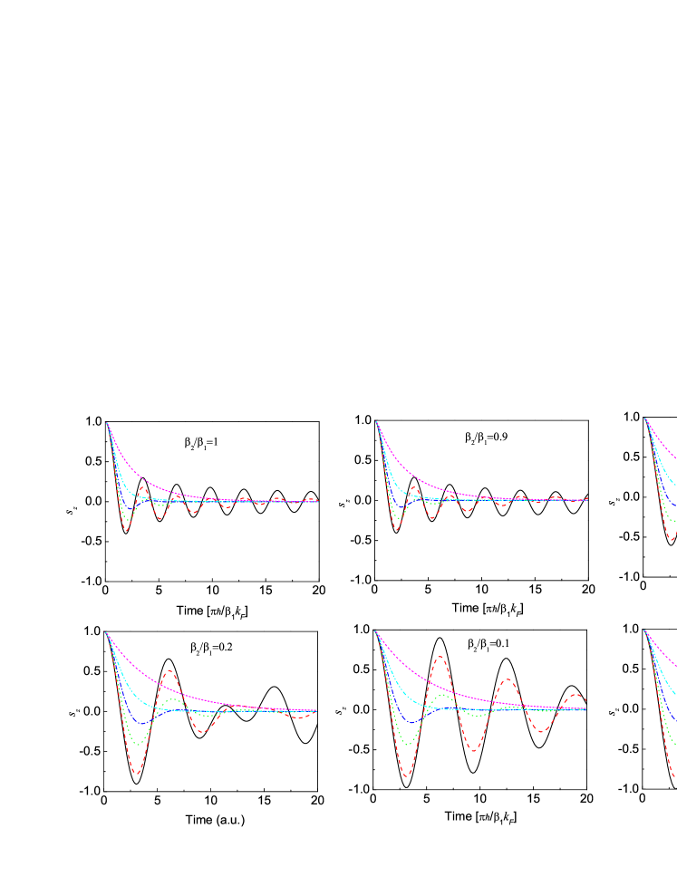
Figure 1: The time dynamics of the average $z$-component of the electron spin for different ratio of BIA and SIA terms for a fixed $\beta_{1}$ term. The time units are $\pi\hbar/\beta_{1}k_{F}$. The ratio $\beta_{2}/\beta_{1}$ is shown above each panel. Various curves correspond to different scattering rates, see legend.

Figure 1 presents the time dependence $s_{z}(t)$ obtained by the numerical solution of Eq. (15). Different panels of Fig. 1 show the results for different ratios $\beta_{2}/\beta_{1}$ calculated at a fixed $\beta_{1}$. Eq. (16) clearly shows that the dependence $s_{z}(t)$ is invariant under the replacement $\beta_{1}\leftrightarrow\beta_{2}$. Different curves in each panel are calculated for different scattering rate $\tau^{-1}$. Even a small admixture of the other term to the strong first term in Hamiltonian (2), e.g. $\beta_{2}/\beta_{1}=0.2$, leads to the damping of the oscillations and quite complicated behavior of $s_{z}(t)$.

The inclusion of the scattering first smears the oscillations. The damping time is non-monotonous function of $\tau^{-1}$ in accordance with the qualitative discussion presented above. For small scattering rates the scattering enhances spin relaxation, while for the stronger scattering the spin dynamics becomes collision dominated and the spin relaxation time becomes longer.

The possibility for the experimental observation of these oscillations depends strongly on the relation between the average spin precession frequency $\bar{\Omega}_{k_{F}}$, scattering time $\tau$ and thermal broadening time $\tau_{T}$. Namely, the condition $\bar{\Omega}_{k_{F}}\tau\gtrsim 1/2$ guarantees the spin precession regime. Moreover, $\bar{\Omega}_{k_{F}}\tau_{T}$ should be larger than unity in order avoid thermal damping of the oscillations.

The dominant broadening mechanism is therefore determined by the shortest of $\tau_{T}$ and $\tau$. For very low temperatures $\tau_{T}$ is very long while $\tau$ is determined by the carrier scattering on the interface roughness and remote impurities. In this regime the beats are damped due to electron elastic scattering. In the regime of the intermediate temperatures where electron-electron scattering dominates over the elastic processes governing the momentum relaxation Leyland et al. (2006), the scattering rate is proportional to $\tau^{-1}\propto k_{B}^{2}T^{2}/\hbar E_{F}$ and scales as $T^{2}$ Glazov and Ivchenko (2004), whereas the thermal broadening rate $\tau_{T}^{-1}\propto\bar{\Omega}_{k_{F}}k_{B}T/E_{F}\propto T$, see Eq. (9). Their ratio $\tau_{T}/\tau$ scales as $k_{B}T/\hbar\bar{\Omega}_{k_{F}}$ and can be both larger or smaller than $1$. For example, in the experimental conditions of Ref. brand02 $\hbar\bar{\Omega}_{k_{F}}\approx 1$ meV and for the temperatures larger than $\hbar\bar{\Omega}_{k_{F}}/k_{B}\approx 12$ K the damping of the beats is due to the electron-electron scattering. We note that in the experiments quasi-equilibrium initial spin distribution can be established during the energy relaxation time $\tau_{E}$ which can be comparable with $\tau$. In such a case one can not separate two contributions to the beats decay.

In the steady-state experiments one measures the spin polarization degree at the continuous spin generation rate. Let us assume that this rate $\bm{G}_{s}$ is directed along $z$-axis and is isotropic in the $\bm{k}$ space. Provided the carrier lifetime is much longer than the spin relaxation time, the stationary solution of Eqs. (10)-(12) reads

$$s_{z,\bm{k}}=\frac{\bar{s}_{z,k}+G_{s}\tau}{1+\Omega_{\bm{k}}^{2}\tau^{2}},$$ (17)

where the average spin-$z$ component is given by

$$\bar{s}_{z,k}=\frac{G_{s}\tau}{[(1+\tilde{\Omega}_{0}^{2}\tau^{2}+2\tilde{\Omega}_{2}^{2}\tau^{2})(1+\tilde{\Omega}_{0}^{2}\tau^{2}-2\tilde{\Omega}_{2}^{2}\tau^{2})]^{\frac{1}{2}}-1}.$$ (18)

We remind that $\tilde{\Omega}_{0}^{2}$ and $\tilde{\Omega}_{2}^{2}$ are defined by Eq. (16). For example, if the spin splitting is isotropic the proportionality coefficient between average spin $\bar{s}_{z}$ and $G_{s}$ is simply given by $(\tilde{\Omega}_{0}^{2}\tau)^{-1}$ which coincides with Dyakonov-Perel’ spin relaxation rate in the collision dominated regime Dyakonov and Perel’ (1972); Dyakonov and Kachorovskii (1986).

IV Spin dynamics in a magnetic field

It is well known that the magnetic field $\bm{B}\parallel z$ slows down the spin relaxation in the collision dominated regime Ivchenko (1973); Glazov (2004). The goal of this Section is to analyze the effects of the magnetic field for the arbitrary relation between $\bar{\Omega}_{k_{F}}$ and $\tau^{-1}$. Here we neglect the non-zero temperature effects.

The magnetic field has a two-fold effect on the spin dynamics. First, it causes the precession of electron spins due to Larmor effect and, second, the cyclotron motion of the electrons in the field leads to the rotation of the wavevector $\bm{k}$ of a given electron and correspondingly the spin precession vector $\bm{\Omega}_{\bm{k}}$. The effects can be taken into account as additional terms in the left hand side of the kinetic equation (1), namely, $\bm{s}_{\bm{k}}\times\bm{\omega}_{L}$ and $\hat{\Lambda}\bm{s}_{\bm{k}}=\bm{\omega}_{C}[\bm{k}\times\partial\bm{s}/\partial\bm{k}]$ with $\bm{\omega}_{L}$ and $\bm{\omega}_{C}$ being the Larmor and cyclotron frequencies respectively, see Ref. Glazov (2004).

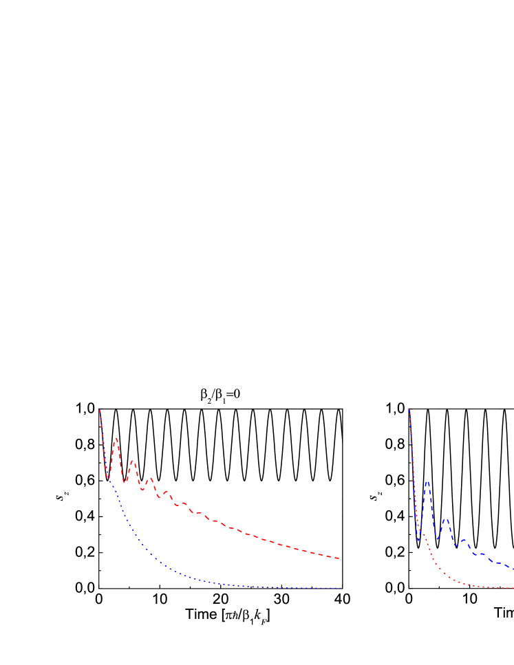
Figure 2: The time dynamics of the average $z$-component of the electron spin in the magnetic field for different values of the scattering rate $\tau^{-1}$, see legend. Left panel: isotropic spin splitting $\beta_{2}/\beta_{1}=0$, right panel: strongest anisotropy $\beta_{2}/\beta_{1}=1$.

First, we start from the clean limit where the scattering is absent and the spin-splitting is isotropic. One can use the rotating frame of reference where the $\bm{\Omega}_{\bm{k}}$ does not rotate. In this frame the electron spin experiences the magnetic field being a sum of three components: $\bm{\Omega}_{\bm{k}}$, $\bm{\omega}_{L}$ and effective field arising due to transition to the non-inertial frame which equals to $\pm\bm{\omega}_{C}$ (upper sign for $\beta_{2}\neq 0$ and lower sign for $\beta_{1}\neq 0$) wilamowski . The spin of the Fermi-surface electron exhibits the harmonic oscillations around the non-zero value $\omega^{2}/(\omega^{2}+\Omega_{k_{F}}^{2})$ with the amplitude $\Omega_{k_{F}}^{2}/(\omega^{2}+\Omega_{k_{F}}^{2})$ and frequency $\sqrt{\omega^{2}+\Omega_{k_{F}}^{2}}$ where $\omega=\omega_{C}\pm\omega_{L}$ (sign depends on the splitting mechanism in question) Glazov and Sherman (2006).

The difference of beats frequencies for BIA and SIA spin splittings in the magnetic field allows, in principle, to determine experimentally the symmetry of the spin splitting. We note that, however, the cyclotron frequency is much larger than the Larmor one, $\omega_{C}\gg\omega_{L}$ in the most conventional systems and we disregard the Larmor effect from now on.

For the anisotropic spin splitting spin beats become anharmonic. Applying Eq. (6) to the case of strongest anisotropy $\beta_{1}=\beta_{2}\equiv\beta$ and taking into account that $\bm{k}$ rotates with cyclotron frequency we obtain for the total spin

$$s_{z}(t)=s_{z}(0)\mathrm{J}_{0}\left(\frac{8\beta k}{\hbar\omega_{C}}\sin{\frac{\omega_{C}t}{2}}\right).$$ (19)

One can see that even a small magnetic field restores the strictly periodic spin dynamics with the period $T=4\pi/\omega_{C}$, i.e. twice larger than the cyclotron one. The time dependence of the total spin is quite non-trivial: the spin beats demonstrate multiple harmonics.

In the presence of the scattering, oscillations decay with time as it is seen from the left panel of Fig. 2. For the anisotropic spin splitting the situation is qualitatively the same, see the right panel of Fig. 2.

If the magnetic field becomes so strong that $\omega_{C}\gg\bar{\Omega}_{k_{F}}$ the variations of the effective field $\bm{\Omega}_{\bm{k}}$ occur on the shorter time-scale than the spin precession in this field. It means that the anisotropic part of the spin distribution $|\bm{s}_{\bm{k}}-\bar{\bm{s}}_{k}|\ll s_{z,k}$. In other words, spin rotation angles between the strong variations of $\bm{\Omega}_{\bm{k}}$ are small. This regime is analogous to the collision dominated regime where the scattering is faster than the spin rotation. Thus, Eq. (1) can be solved by iterations and the total spin decays exponentially with the time-constant

$$\tau_{s}=(1+\omega_{C}^{2}\tau^{2})/\tilde{\Omega}_{0}^{2}\tau,$$ (20)

where $\tilde{\Omega}_{0}$ is given by Eq. (16). We underline that Eq. (20) (as well as the results of Ref. Glazov (2004)) is valid for the arbitrary relation between $\bar{\Omega}_{k_{F}}$ and $\tau^{-1}$ provided the magnetic field is strong enough.

The results presented above are derived for the case of the isotropic scattering, where all the angular harmonics of the distribution functions relax with the same time-constant $\tau_{m}=\tau$ (for $m=1,2,\ldots$). Qualitatively, these results hold true for the case of angular dependent scattering. Numerical solution of Eq. (1) in the limiting case of the long-range classical potential, where the collision integral can be replaced by differential operator $\bm{Q}_{\bm{k}}\{\bm{s}_{\bm{k}}\}=-\tau^{-1}\partial^{2}\bm{s}_{\bm{k}}/\partial\varphi_{\bm{k}}^{2}$, shows almost no difference with the presented results.

In conclusion, we have theoretically analyzed the spin dynamics of the two dimensional electron gas in asymmetrical QWs for the arbitrary relation between the scattering rate and the spin precession rate at low temperature regime. We have demonstrated that the spin dynamics shows quite complicated beats for the anisotropic spin splitting. In this case the beats decay due to the spread of the spin precession frequencies. The suppression of the beats by the thermal smearing of the distribution function, carrier scattering and the magnetic field has been studied.