Collective coherence in planar semiconductor microcavities

Abstract

Semiconductor microcavities, in which strong coupling of excitons to confined photon modes leads to the formation of exciton-polariton modes, have increasingly become a focus for the study of spontaneous coherence, lasing, and condensation in solid state systems. This review discusses the significant experimental progress to date, the phenomena associated with coherence which have been observed, and also discusses in some detail the different theoretical models that have been used to study such systems. We consider both the case of non-resonant pumping, in which coherence may spontaneously arise, and the related topics of resonant pumping, and the optical parametric oscillator.

1 Introduction

Semiconductor microcavities have been designed to greatly enhance the matter-light interaction strength by confining light. The confined light couples to excitonic resonances in the medium inside the microcavity; when this exciton-photon coupling exceeds the exciton and photon damping rates one finds spectrally separated normal modes, microcavity exciton-polaritons [1, 2]. Unlike many other examples of strong coupling, studied in quantum optics, this review will focus on planar semiconductor microcavities that confine photons in only one direction, thus leading to a continuum of strongly coupled modes. Due to their dual matter-light nature, exciton polaritons can be manipulated and studied through their light component, and have an effective interaction through their matter component and the nonlinearity of light-matter coupling. Due to the continuum of modes, the behaviour of exciton polaritons may be related to the statistical mechanics of interacting bosons. Thus, semiconductor microcavities provide an ideal system in which to study the interface between quantum optics, strong coupling, spontaneous coherence and quantum condensation.

A closely related area of research, although one we will not address in this review, is strong coupling to single excitonic resonances i.e. excitons in quantum dots in semiconductor microcavities. As well as experiments on quantum dots in planar microcavities [3], experiments with confinement of photons in either three or two spatial directions are also performed. In the first case, 0D microcavities have been constructed from photonic crystals [4, 5] (in which in-plane confinement results from localisation on a defect in the photonic crystal, and vertical confinement from total internal reflection), as well as micropillars [6] (where Bragg mirrors provide vertical confinement, and total internal reflection provides in-plane confinement). In the second case, wire structures were fabricated by chemical etching [7]. Lying between confinement in one and three spatial directions are experiments in patterned microcavities, where schematically a variation in the width of the microcavity provides a shallow in-plane trap for photon modes [8, 9, 10]. This results in coexistence of 0D and 2D polariton states, separated in energies: A clear polariton spectrum has been seen along with the quantisation induced by a box-like confinement. Polariton localisation due to the intrinsic photonic disorder has also been observed [11].

Our review will concentrate on macroscopic collective phenomena arising from the interaction between these special bosonic particles. While some of these issues have been addressed in other contexts — such as quantum condensation in dilute atomic gases [12, 13], and coherent quantum optics of lasers [14] — the combination of effects seen in microcavity polaritons calls for new approaches. In part, the new theoretical challenges arise from description of features of semiconductor microcavities, such as the disorder and decoherence that arise in solids, the spin structure of polaritons, and the effect of pumping and decay. In addition, polariton systems provide new opportunities for experimental probes and observations that differ from those possible in other systems.

The recent experimental and theoretical research in this field can be divided into two main directions: Firstly, experiments which use resonant (coherent) pumping have been motivated by the search for all-optical ultrafast switches and amplifiers. The other direction is that of non-resonantly pumped microcavities, where experiments have pursued the search for Bose-Einstein condensation (BEC), polariton lasing and macroscopic phase coherence phenomena.

A number of reviews have been already written on the subject of microcavity polaritons: In Refs. [15, 16], linear properties of microcavities have been analysed in great detail. Refs. [17, 18] review problems of non-linear optics and the theoretical framework necessary to study resonant pumping, parametric amplification and oscillation. In addition, two books [19, 20] and two special issues [21, 22] have also been published. In this review, we will focus attention on those issues of modelling microcavity polaritons that are of particular importance in understanding spontaneous coherence and condensation in such systems. We will address the relation between the various theoretical approaches that have been used, and discuss the limits in which they become equivalent. We will also discuss in some detail the relation between coherence, condensation, lasing and superfluidity in experimental systems which are finite, two-dimensional, decaying, and interacting, and thus differ from the Bose-Einstein condensation of ideal three-dimensional bosons. Finally, we will discuss the relation of these features both to the resonantly pumped polariton system, and also to other experimental systems in which similar issues of coherence and condensation in complex systems are addressed.

The review is divided overall into non-resonant pumping in Sec. 2 and resonant pumping in Sec. 3. Within Sec. 2, we first present the experimental development of the subject in Sec. 2.1, and then discuss the theoretical approach, dividing our discussion into the question of choice of model in Sec. 2.2, choice of treatment (i.e. thermal equilibrium, rate equations, etc.) in Sec. 2.3, and the phenomena predicted (i.e. experimental signatures, conditions for condensation) in Sec. 2.4. Within Sec. 3 we again divide into a summary of experimental progress in Sec. 3.1, and a discussion of the additional theoretical issues relevant only to the resonantly pumped case in Sec. 3.2. Section 4 finally draws comparisons to phenomena seen in other experimental systems, and briefly summarises our discussion.

1.1 Introduction to microcavity polaritons

Before discussing experiments and theories of coherence in microcavity polaritons, we provide here a brief introduction to the systems considered, and to microcavity polariton modes. Fuller introductions can be found elsewhere [23, 19, 20]. The semiconductor microcavities we discuss are constructed from distributed Bragg reflectors, containing alternating quarter wavelength thick layers of dielectrics with differing refractive indices. Due to these Bragg reflectors, the cavity contains a standing wave pattern of confined radiation. As illustrated in Fig. 1, quantum wells (QWs) are placed at the antinodes of this standing wave, thus maximising the coupling between photons and excitons confined to the quantum wells.

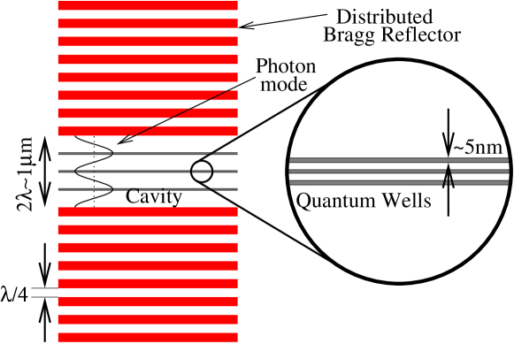
Figure 1: Schematic diagram of a microcavity, formed by a pair of distributed Bragg reflector stacks, with quantum wells at the antinodes of the cavity photon mode.

Because the photon modes are confined to the cavity, the volume associated with the radiation mode is small, and so the exciton-photon coupling is strong. This strong coupling means that rather than considering the exciton-photon coupling as leading to radiative decay of the excitons, the exciton and photon modes are instead mixed, to form new normal modes: lower and upper polaritons. At the simplest level, one can write the exciton-photon Hamiltonian in terms of operators $\psi_{\mathbf{k}}^{\dagger}$ creating photons and $D_{\mathbf{k}}^{\dagger}$ creating excitons, with $\mathbf{k}$ labelling the 2D in-plane momentum. Thus:

$$H=\left(\psi_{\mathbf{k}}^{\dagger},D^{\dagger}_{\mathbf{k}}\right)\left(\begin{array}[]{cc}\omega_{\mathbf{k}}&\Omega_{R}/2\\ \Omega_{R}/2&\varepsilon_{\mathbf{k}}\end{array}\right)\left(\begin{array}[]{c}\psi_{\mathbf{k}}\\ D_{\mathbf{k}}\end{array}\right).$$ (1)

[We have set $\hbar=1$ here and throughout.] Here, $\omega_{\mathbf{k}}$ is the energy of the photon mode confined in the cavity of width $w$, giving: $\omega_{\mathbf{k}}=(c/n)\sqrt{k^{2}+(2\pi N/w)^{2}}$, with $n$ is the refractive index, and $N$ the index of the transverse mode in the cavity. For the situation in Fig. 1, $N=2$. For small $k$, the energy can be written as $\omega_{\mathbf{k}}=\omega_{0}+k^{2}/{2m}$, where $m$ is an effective photon mass $m=(n/c)(2\pi/w)$. In the absence of disorder, the exciton energy in the QW is $\varepsilon_{\mathbf{k}}=\varepsilon_{0}+k^{2}/2M$, where $M$ is the total exciton mass, and $\varepsilon_{0}=E_{cv}-\mathcal{R}_{ex}$ comes from the conduction-valence band gap $E_{cv}$ including QW confinement and the exciton binding energy (Rydberg) $\mathcal{R}_{ex}$. For convenience, we define the bottom of the exciton band, $\varepsilon_{0}$ as the zero of energies; and denote the detuning between exciton and photon bands as $\delta=\omega_{0}-\varepsilon_{0}$. Finally, the off diagonal term $\Omega_{R}/2$ describes the exciton-photon coupling, where $\Omega_{R}$ is the Rabi frequency. Then, diagonalising the quadratic form in Eq. (1) gives the polariton spectrum:

$$E_{\mathbf{k}}^{\mathrm{LP},\mathrm{UP}}=\frac{1}{2}\left[\left(\delta+\frac{k^{2}}{2M}+\frac{k^{2}}{2m}\right)\mp\sqrt{\left(\delta+\frac{k^{2}}{2M}-\frac{k^{2}}{2m}\right)^{2}+\Omega_{R}^{2}}\right].$$ (2)

This spectrum is illustrated in Fig. 2. It is shown there both as a function of momentum $k$, and also as a function of angle. The angle corresponds to the angle of emission of a photon out of the cavity; since the in-plane momentum and photon frequency are both conserved as photons escape through the Bragg mirrors, one may write $(\varepsilon_{0}+E^{LP}_{\mathbf{k}})\sin(\theta)=ck$, which (since typical values of $k$ satisfy $\omega_{0},\varepsilon_{0}\gg ck$) can be approximated as $\omega_{0}\sin(\theta)=k^{2}/2m$.

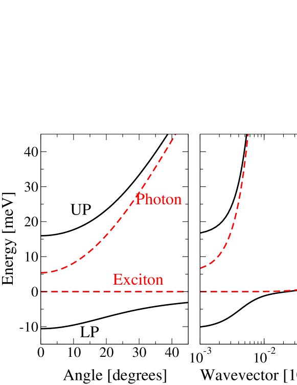
Figure 2: Schematic polariton spectrum. Left as a function of emission angle, $\theta=\sin^{-1}(ck/\omega_{0})$; Right, as a function of momentum on a logarithmic scale, showing the full exciton dispersion. (Plotted for $M=0.08m_{e}$, $m=3\times 10^{-5}m_{e}$, $\Omega_{R}=26$meV, $\delta=5.4$meV and $\omega_{0}=1.7$eV.)

2 Non-resonant pumping

2.1 Summary of experiments

Optical properties of semiconductor microcavities have been the subject of extensive experimental investigations since the first observation of the strong coupling regime by Weisbuch et al. [2]. Much of the experimental research has concentrated on III-V materials, mainly GaAs/AlGaAs structures, or on II-VI materials, such as CdTe/CdMnTe/CdMgTe structures. The main aim of the experiments described here as non-resonant pumping has been to start with incoherently injected polaritons, and observe spontaneous coherent processes emerging from incoherent injection of polaritons: polariton degeneracy, final state stimulation, and ultimately polariton BEC.

The authors of the earliest report [24] of non-linear emission in the presence of strong coupling in GaAs microcavities, suggesting final state stimulation characteristic for bosonic particles, later withdrew those conclusions [25] as further experiments showed that the threshold for non-linear emission occurred in that case after the crossover to the weak-coupling regime; thus the non-linear emission should have been attributed to photon lasing. The first unambiguous observation of polariton bosonic stimulation was in CdTe microcavities [26] consisting of 16 quantum wells with a Rabi splitting of around $23$meV. Two distinct stimulation thresholds were observed with increasing intensity of continuous wave pumping, as shown in Fig. 3. As the pumping intensity was increased above the first threshold, non-linear emission at energies close to the bottom of the lower polariton branch was clearly seen. The second threshold, reported for much higher intensities, was connected with a weak coupling electron-hole lasing mechanism. Further investigation [27, 28] showed that the first nonlinear threshold — in the strong coupling regime — was due to stimulated scattering to the ground state. Very shortly after publication of Ref. [26], non-linear emission was seen in a single QW GaAs microcavity [29], characterised by 3.5meV Rabi splitting. However further investigation [30] showed that this nonlinearity had emission varying as the square of pumping intensity, and a threshold that occurred for occupation factors much less than one, and so this nonlinearity was associated with increase of exciton-exciton scattering, rather than final state stimulation. Final state stimulation in III-V materials was demonstrated by pump-probe experiments in Refs. [30, 31].

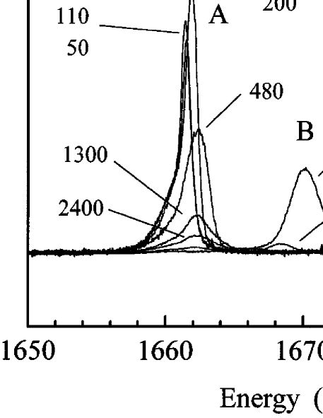
Figure 3: Panel (a): Reflectivity spectrum, showing location of lower and upper polariton modes in the absence of pumping. Panel (b): Photoluminescence as pumping power is increased, a threshold for nonlinear emission is seen at $40$kW/cm², while the system clearly remains in the strong coupling regime. In panel (c), at much higher pumping powers ($10,000$kW/cm²), a second threshold, to electron-hole lasing is seen. [From [26] Copyright (1998) by the American Physical Society]

The stimulated scattering to the ground state, and non-linear build-up of lower polariton population was the first step towards demonstration of spontaneous coherence and thermalisation — characteristic of quantum condensation. However, the big challenge to realising a condensed polariton phase was the finite (though very large) quality of the cavity mirrors, and the resultant short polariton lifetime, of the order of picoseconds. In addition, due to the ‘bottleneck effect’, [32] the relaxation of polaritons to the zero momentum state was delayed, hindering the creation of a thermal population in the lowest energy states. The first investigation of the coherence properties of emitted light above the threshold for non-linear emission in strong coupling was based on the measurement [33, 34] of the second order coherence function, $g_{2}(t=0)$, which would take a value of $g_{2}(0)=2$ for a thermal state, and $g_{2}(0)=1$ for a coherent state [35]. A decrease of $g_{2}(0)$ from $1.8$ to $1.4$ as pumping power was increased from threshold to $20$ times threshold power was seen in a system of $12$ GaAs quantum wells placed at the antinodes of light in a GaAs/AlGaAs microcavity, giving $14.9$meV Rabi splitting. This was followed by a report of a characteristic change in the momentum space distribution above threshold [36], as shown in Fig. 4, and a blueshift of the polariton dispersion [37]. Time-resolved photoluminescence measurements were also performed for a CdTe microcavity with $10.5$meV Rabi splitting [38] under non-resonant pulsed excitation, which were able to monitor the buildup of a large polariton population in the $\mathbf{k}=0$ state. Analysis of the time dependence showed that, below threshold, the dynamics of the $\mathbf{k}=0$ polaritons follows closely the population of cold reservoir excitons; the relaxation from high energy exciton states resonant with the pump to these reservoir exciton states had a characteristic relaxation time of $30$ps. [Note that this time is significantly shorter than the $150$ps observed in similar experiments [39] with GaAs based microcavities.] Above the non-linear threshold, the population of the reservoir excitons was found to be clamped, and the polariton relaxation dynamics became faster, with the maximum of polariton emission at $70$ps delay after the initial pulse. This delay was further decreased for higher excitations powers. Together these provide evidence of stimulated exciton-exciton scattering to the lower polariton states.

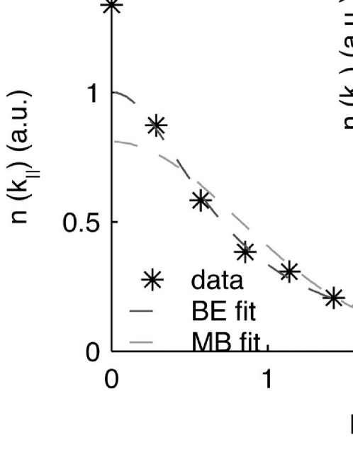
Figure 4: Momentum space distribution of lower polaritons above (main figure) and below (inset) the nonlinear threshold. [From Ref. [36], Copyright 2003 National Academy of Sciences]

The first evidence of spontaneous first-order coherence in an incoherently pumped microcavity was seen in a 16 QW CdTe microcavity with 26meV Rabi splitting [40] under non-resonant pulsed pumping. An interesting feature of this particular experiment was that the non-linear emission was at $\mathbf{k}\neq 0$ and so resulted in an emission ring at an angle of around $17^{\circ}$; this was associated with the small size of the excitation spot (3 $\mu$m). (Note that in later experiments with larger excitation spots on the same sample condensation was at $\mathbf{k}=0$ [41].) The first-order coherence was investigated by spectroscopic imaging of the far-field emission. Two momentum space images were superimposed giving fringes (as a function of momentum $\mathbf{k}$) with over 75$\%$ contrast above threshold and up to 35$\%$ below threshold. In a later publication of the same group [42], experiments on a 4 QW CdTe microcavity characterised by $13.2$meV Rabi splitting showed macroscopic occupation of the $\mathbf{k}=0$ state characterised by narrowing above threshold of the polariton emission line to a linewidth below that of the cavity photon mode. Near-field images showed modulation of the polariton spatial distribution, revealing the effect of photonic disorder. The next challenge in the search for spontaneous condensation was to see similar effects, but accompanied by a thermal distribution of $\mathbf{k}\neq 0$ polaritons.

Due to the short polariton lifetime and the ‘bottleneck effect’, [32] the realisation of equilibrium population has proven to be challenging. Progress came from observing [43, 41] that thermalisation processes due to particle-particle scattering can be dramatically increased both by increasing the value of the (non-resonant) pump power, and also by positively detuning the cavity energy above the excitonic energy. Large positive detuning makes polaritons more excitonic and increases their scattering rate. Time- and angle-resolved spectroscopy on a sample consisting of 12 GaAs QWs characterised by 14.4meV Rabi splitting [43] showed that for positively detuned cases, where the thermalisation time increases while decay time decreases, the thermalisation time can reach around one tenth of the polariton lifetime and that lower polaritons remain in thermal equilibrium with the phonon bath for a period of about 20ps. Finally, a comprehensive set of experiments showing clear evidence for condensation of cavity polaritons was performed in a CdTe [41] structure consisting of 16 quantum wells giving 26meV Rabi splitting. Above the threshold pumping density they observed: a massive occupation of the $\mathbf{k}\cong 0$ mode developing from a polariton gas in thermal equilibrium at 19K (shown in Fig. 5); an increase of temporal coherence from $1.5$ps below threshold to up to $6$ps above threshold; the build-up of long-range spatial coherence over the whole system size with contrast of interference fringes from less than 5$\%$ below threshold to 45$\%$ above threshold; linear polarisation of the emission. Linear polarisation had been predicted to appear in the condensed state [44], and its appearance gives evidence for the single state nature of the condensate, though since the direction of this polarisation was pinned to a crystallographic direction the polarisation direction symmetry was not spontaneously broken. Evidence that the polarisation of light is pinned to one of the crystallographic axes, independently of the excitation polarisation, was also independently observed in experiments on both CdTe [45] and InGaAs microcavities [46]. These results were ascribed to birefringence in the mirrors and cavity. Shortly following the work in Ref. [41], a similar non-linear build up accompanied by a linear polarisation was seen [47] in GaAs structures in stress-induced traps [48]. Also the second order coherence function, $g_{2}(t=0)$, has been measured [49] in the CdTe structures studied in Ref. [41] where, in contrast to observations reported in Ref. [33], $g_{2}(0)$ was found to be around 1 at threshold and then increased up to around 1.4 at powers 10 times threshold. This effect has been attributed to the phase diffusion due to interactions.

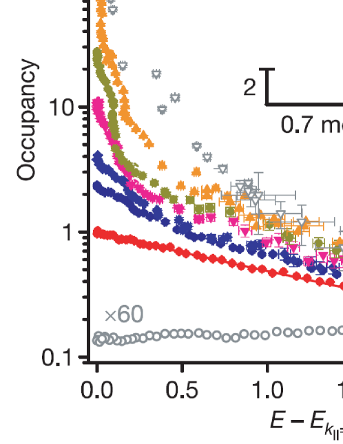
Figure 5: Polariton occupation vs energy, showing evolution from below to above threshold power, with the distribution remaining thermalised at a temperature of $19K$ [From Ref. [41]]

Wide-band-gap semiconductor structures based on group-III nitrides, such as GaN based cavities have recently attracted considerable interest (see, e.g., [50, 51, 52, 53, 54, 55, 56, 57]). The main advantage of these structures over II-VI and other III-V materials lies in the large exciton binding energy (around $26$meV for bulk structures, and over $40$meV for narrow quantum wells) and the large coupling to the photon field, which makes them ideal systems for the realisation of functional devices operating at room temperature. Although the study of cavity polaritons in group-III nitrides microcavities is still in its infancy, strong exciton-photon coupling in a bulk GaN cavity [50, 53, 51] and in a quantum well cavity [54] have been reported. In both cases, the substantial inhomogeneous broadening of the excitonic and photonic lines play a key role in establishing the conditions for reaching strong coupling. Very recently, a non-linear build-up of polariton emission accompanied by an increase in the first-order temporal coherence, and a spontaneously chosen linear polarisation (independent of the apparatus and different between measurements) has been reported to occur at room temperature in GaN bulk microcavities [58].

2.2 Theoretical models

In this section, we will discuss the different models that have been used to describe microcavity polaritons and study their condensation. We wish to separate clearly two aspects of theoretical description of polaritons; the first aspect is the choice of model, the subject of this section, the second aspect is how that model is treated, which will instead be covered in Sec. 2.3. After having addressed these points, we then in Sec. 2.4 discuss the various theoretical predictions of conditions for condensation, and of possible signatures. Readers who are not interested in the details of how the system is theoretically modelled should jump to Sec. 2.4. A model starting from electrons and holes, taking into account their Coulomb interaction to form bound excitons, their coupling to light, and the effects of disorder would describe polariton systems exactly, but is too complicated to allow any clear understanding of the important features associated with condensation to be gained. Therefore, it is appropriate to use simplified models, that exaggerate some features of the real system, and neglect others. In judging which model is appropriate to address a given problem, it is important to understand how the model relates to the underlying microscopic model of electrons and holes, and so we shall start by discussing this microscopic model.

2.2.1 Microscopic electron-hole Hamiltonian

In this section, we discuss the underlying description of microcavity polaritons formed from photons confined to a two-dimensional cavity, interacting with electrons and holes in two-dimensional quantum wells [59, 23].

$$H=H_{\mathrm{eh}}+H_{\mathrm{coul}}+H_{\mathrm{disorder}}+H_{\mathrm{photon}}+H_{\mathrm{dipole}}$$ (3)

Consider first the electrons and holes, we have

$$H_{\mathrm{eh}} = \sum_{\mathbf{k}}\varepsilon^{c}_{\mathbf{k}}c^{\dagger}_{\mathbf{k}}c_{\mathbf{k}}+\varepsilon^{v}_{\mathbf{k}}v^{\dagger}_{\mathbf{k}}v_{\mathbf{k}}$$ (4)

$$H_{\mathrm{coul}} = \frac{1}{2A}\sum_{\mathbf{q}}\frac{e^{2}}{2\epsilon_{r}\epsilon_{0}|\mathbf{q}|}\left[\rho^{e}_{\mathbf{q}}\rho^{e}_{-\mathbf{q}}+\rho^{h}_{\mathbf{q}}\rho^{h}_{-\mathbf{q}}-2\rho^{e}_{\mathbf{q}}\rho^{h}_{-\mathbf{q}}\right]$$ (5)

$$H_{\mathrm{disorder}} = \int d\mathbf{r}\left[W_{e}(\mathbf{r})c^{\dagger}(\mathbf{r})c(\mathbf{r})-W_{h}(\mathbf{r})v(\mathbf{r})v^{\dagger}(\mathbf{r})\right]\;.$$ (6)

Here $c^{\dagger}_{\mathbf{k}}$ ($v^{\dagger}_{\mathbf{k}}$) create electrons in the conduction (valence) bands, which have dispersions, $\varepsilon^{c}_{\mathbf{k}}$ ($\varepsilon^{v}_{\mathbf{k}}$). Since the “empty” state is a filled valence band, it is more convenient to describe the valence band via the operator $v_{\mathbf{k}}$ which creates a hole — i.e. a missing electron. The density of electrons (holes) is given by $\rho^{e}_{\mathbf{q}}=\sum_{\mathbf{k}}c^{\dagger}_{\mathbf{k}+\mathbf{q}}c_{\mathbf{k}}$ ($\rho^{h}_{\mathbf{q}}=\sum_{\mathbf{k}}v_{\mathbf{k}}v^{\dagger}_{\mathbf{k}+\mathbf{q}}$). The factor $1/A$, where $A$ is the quantisation area of the cavity, appears explicitly because the Hamiltonian has been written as a sum over momentum labels; this factor plays no role in any final answer, and is absorbed in the definition of $d\mathbf{k}$ if summation is replaced by integration. Note also that in general there should be a dependence on the electron and hole spin degrees of freedom, that we neglect here. The last term, Eq. (6), describes the disorder potential acting on electrons and holes, e.g. due to well-width fluctuations and alloy disorder. In general, disorder can act differently on electrons and holes; in practice for the materials used, the energy scale of disorder is less than the binding energy, so disorder does not dissociate excitons [60]. If the exciton binding energy is significantly larger than a characteristic energy scale of disorder, then as described in Ref. [60] one can factorise the wavefunction into a centre of mass wavefunction, and a wavefunction of relative electron-hole separation. Then, in the equation for the centre of mass wavefunction, one has an effective disorder potential that is the result of convolving the original disorder with the wavefunction for relative electron-hole separation. As a result of this convolution, the effective disorder potential as seen by the exciton centre of mass wavefunction is smoothed over the scale of the exciton Bohr radius [61].

Turning now to the interaction with the photons,

$$H_{\mathrm{photon}} = \sum_{\mathbf{q}}\omega_{\mathbf{q}}\psi^{\dagger}_{\mathbf{q}}\psi_{\mathbf{q}}+\int d\mathbf{r}W_{\mathrm{ph}}(\mathbf{r})\psi^{\dagger}(\mathbf{r})\psi(\mathbf{r})$$ (7)

$$H_{\mathrm{dipole}} = \frac{1}{\sqrt{A}}\sum_{\mathbf{q},\mathbf{k}}e\mu_{cv}\sqrt{\frac{\omega_{\mathbf{q}}}{2\epsilon_{r}\epsilon_{0}L_{w}}}\left(\psi_{\mathbf{q}}^{\dagger}v^{\dagger}_{\mathbf{k}+\mathbf{q}}c_{\mathbf{k}}+\mathrm{H.c.}\right)$$ (8)

In Eq. (8), the quantisation volume for the electromagnetic field has been factored into $AL_{w}$, where $L_{w}$ is the width of the cavity, and $A$ the quantisation area as discussed above. The term $\mu_{cv}$ is the inter-band dipole matrix element, which can be calculated given the Bloch wavefunctions of the two bands. The term $W_{\mathrm{ph}}(\mathbf{r})$ in Eq. (7) describes photonic disorder, which can arise due to roughness of the Bragg mirrors — i.e. due to layer width fluctuations (monolayer mismatch), or crystal dislocations [11, 62]. The effects of this photonic disorder, and of the exciton disorder introduced above, can be quite different. The photonic disorder is generally on large length scales (typically of the order of a micrometre), comparable to the size of the excitation spot, and so it is primarily associated with the spatial inhomogeneity of polaritons seen in experiment [42]. In contrast, as discussed in Sec. 2.2.3, excitonic disorder is on much shorter length scales (typically of the order of ten nanometres for CdTe), and thus does not affect the spatial polariton density profile; however excitonic disorder does have a significant impact on the distribution of excitonic oscillator strengths. Although the excitons are localised, in the absence of photonic disorder the polaritons formed consist of a superposition of many different localised excitons and extended photon states, and thus one may form delocalised polaritons from localised excitons [63]. We will not explicitly discuss the effects of photonic disorder further, however the discussion of condensation in a trap in Sec. 2.3.3 can apply also to trapping in disorder, as well as any deliberately engineered trapping.

The Hamiltonian in Eq. (3) already contains a number of important approximations, which should be discussed. The interaction of photons with electrons and holes makes use of both the dipole approximation, and the rotating wave approximation [23, Chapter 10]. The interaction strength here is written in the dipole (length) gauge. The choice between the dipole (length) gauge and the Coulomb (velocity) gauge is not arbitrary, as the terms assigned as describing free particles (without interaction with radiation) are different in each gauge [64, 65, 66]. This point is worth stressing, as the electromagnetic interaction between excitons is split between the direct Coulomb term, and a photon mediated term. Thus the choice of gauge affects also the Coulomb interaction [Eq. (5)], controlling which parts of it are absorbed into the definition of exciton states, which parts are associated with the “photon” operators — in the Dipole gauge, the fields $\psi^{\dagger}_{\mathbf{q}}$ are quantised modes of the electric displacement — and which should be written as some effective exciton-exciton interaction [66]. The relation between Coulomb interaction and photon mediated interaction is complicated here because the resonant photons are confined by the DBR (distributed Bragg reflector) mirrors, while the static Coulomb term is modified much less strongly by the mirrors. When one comes to exciton states, it is therefore important to be aware that the choice of gauge affects both the exciton-photon coupling strength, and the form of the inter-exciton Coulomb interaction, and that these two are not separate.

In the next two sections, we will discuss the main two classes of effective Hamiltonians, derived from this full Hamiltonian, used to study microcavity polaritons. The differences between these effective Hamiltonians can be seen as the result of regarding different terms as important; i.e. which terms are treated exactly, and which perturbatively. In both cases, the first step involves changing from electrons and holes to bound excitons — i.e. solving the wavefunction for the relative coordinates. The differences then arise from considering in one case next the effect of disorder, giving localised states, and then approximating the inter-exciton Coulomb term by exclusion — this leads to the boson-fermion model discussed in Sec. 2.2.3 — or alternatively, treating the Coulomb term via a quartic exciton-exciton interaction term, then coupling to light, and then treating disorder perturbatively or not at all — this leads to the weakly interacting boson model, discussed in Sec. 2.2.2.

As will be discussed further below, in the low density limit, many features of these models are similar. However, the different models emphasise different features: The boson model can effectively describe the case where the dominant interactions are exciton-exciton Coulomb interactions, while the boson-fermion model instead has the saturation of the exciton-photon coupling as the dominant interaction. As such, these different models may be appropriate in different contexts. For example, to describe the lower polariton blue-shift, and comparable upper polariton red-shift seen, e.g. in Refs. [41, 49], the effects of the saturation interaction are required. Further, the different models have been developed in different directions, for example the effects of exciton spin, and thus the polarisation dynamics have so far only been considered in the bosonic model (see e.g. Refs. [67, 44] and Refs. therein).

2.2.2 Weakly interacting boson models

A weakly interacting Bose gas model of polaritons can be achieved by making an Usui transformation [68, 69], choosing the bosonic operators to represent bound exciton states, and then truncating the interaction terms at fourth order [70]. This results in an effective Hamiltonian describing bosonic excitons coupled to photon modes:

$$H = \sum_{\mathbf{k}}\left[\omega_{\mathbf{k}}\psi^{\dagger}_{\mathbf{k}}\psi_{\mathbf{k}}+\varepsilon_{\mathbf{k}}D^{\dagger}_{\mathbf{k}}D_{\mathbf{k}}+\frac{\Omega_{R}}{2}(D^{\dagger}_{\mathbf{k}}\psi_{\mathbf{k}}+\psi^{\dagger}_{\mathbf{k}}D_{\mathbf{k}})\right]$$ (9)

$$- \frac{\Omega_{R}}{2\rho_{sat}}\sum_{\mathbf{k},\mathbf{k}^{\prime},\mathbf{q}}\left[D^{\dagger}_{\mathbf{k}^{\prime}-\mathbf{q}}D^{\dagger}_{\mathbf{k}+\mathbf{q}}D_{\mathbf{k}}\psi_{\mathbf{k}^{\prime}}+\psi^{\dagger}_{\mathbf{k}^{\prime}-\mathbf{q}}D^{\dagger}_{\mathbf{k}+\mathbf{q}}D_{\mathbf{k}}D_{\mathbf{k}^{\prime}}\right]$$

$$+ \sum_{\mathbf{k},\mathbf{k}^{\prime},\mathbf{q}}\frac{U_{\mathbf{k}-\mathbf{k}^{\prime},\mathbf{q}}}{2}D^{\dagger}_{\mathbf{k}+\mathbf{q}}D^{\dagger}_{\mathbf{k}^{\prime}-\mathbf{q}}D_{\mathbf{k}^{\prime}}D_{\mathbf{k}},$$

Here $D^{\dagger}_{\mathbf{k}}$ creates a bound exciton of energy $\varepsilon_{\mathbf{k}}$, $\psi^{\dagger}_{\mathbf{k}}$ creates a cavity photon of energy $\omega_{k}$, and $\Omega_{R}$ is the effective exciton-photon coupling strength, or Rabi splitting. By measuring energies from the bottom of the exciton dispersion, we may write $\varepsilon_{\mathbf{k}}=k^{2}/2M$, and expanding the photon dispersion to quadratic order in momentum, one may approximate $\omega_{\mathbf{k}}\simeq k^{2}/2m+\delta$, with $\delta$ the exciton-photon detuning. The quartic terms in Eq. (9) are divided into exciton-exciton interactions, $U_{\mathbf{k}-\mathbf{k}^{\prime},\mathbf{q}}$, the strength of which can also be found by calculation of the Coulomb exchange term [71, 72] in the Born approximation, and a “saturation term”(second line), which decreases the exciton-photon coupling at large exciton densities due to the fermionic character of the excitons [70]. These quartic terms arising from the Usui transformation can be seen as an expansion of the underlying fermionic operators in powers of bosonic operators; this expansion is controlled by the small parameter of the number of excitons per Bohr radius. Note that in general these terms depends also on the spin degrees of freedom of the constituent electron and holes. For a derivation of the dependence on spin of the Coulomb terms, see, e.g., Refs. [73, 74].

This approach takes into account the intra-exciton Coulomb term, in forming bound excitons, and the inter-exciton Coulomb terms as an effective quartic interaction. The Hamiltonian in Eq. (9) however neglects disorder acting on the exciton states, and as a result finds that each exciton state couples to a single photon state, with conserved momentum. However, as discussed below in Sec. 2.2.3, and in Refs. [75, 76], exciton disorder will modify this picture. Including disorder, one finds a distribution of energies, and at each energy a distribution of exciton-photon coupling strengths. The exciton states which have the largest coupling strength to the low momentum photons are found to be at energies just below the exciton dispersion edge. Although these states are not the most localised, i.e. are not the states far in the Lifshitz tail (see later Sec. 2.2.3), they are below the band edge and therefore are still quite strongly localised, they decay quickly at long distances, and they result from exciton wavefunctions concentrated around minima of the potential. The low energy polariton modes will be formed from a superposition of many such localised exciton states.

In addition, the saturation term in this model, which describes the reduction of exciton-photon coupling is taken only to the lowest order. This is sufficient at low enough densities; however as discussed more fully in Sec. 2.2.3, including effects of disorder the density at which these saturation effects become important can be much lower than the Mott density. Thus, a quartic description of saturation may become inadequate at modest densities, close to those already studied experimentally. In addition, most bosonic models of polaritons further simplify Eq. (9), replacing the momentum dependent interaction $U_{\mathbf{k}-\mathbf{k}^{\prime},\mathbf{q}}$ with its strength at $\mathbf{k}=\mathbf{k}^{\prime},\mathbf{q}=0$. This strength is the interaction between two excitons in the same single particle momentum eigenstate. If exciton eigenstates are localised, it is not obvious that replacing all exciton-exciton Coulomb interactions with an average strength (calculated from delocalised exciton wavefunctions) is appropriate. In addition, the dominant Coulomb interaction between localised, and therefore non-overlapping, exciton states may well be due to the direct dipole-dipole interaction, rather than exchange terms (as it is in the clean case). The boson-fermion model discussed Sec. 2.2.3 handles this interaction differently — it includes strong on-site repulsion, and neglects inter-site repulsion; this limit is clearly also an exaggeration, and the true effects of Coulomb will be between these two extremes.

It is worth noting parenthetically that a constraint on exciton density $\sum_{\mathbf{k}}\langle D_{\mathbf{k}}^{\dagger}D_{\mathbf{k}}^{\vphantom{\dagger}}\rangle<\rho_{sat}$ is required to make the Hamiltonian in Eq. (9) stable. Without such a constraint the free energy is unbounded from below, i.e. for $\left|\Psi\right>=\exp\left(\lambda\psi^{\dagger}_{0}+\beta D^{\dagger}_{0}\right)\left|0\right>$, the free energy $F=\left<H-\mu N\right>$ corresponding to Eq. (9) is

$$F=(\delta-\mu)|\lambda|^{2}-\mu|\beta|^{2}+\Omega_{R}\Re(\lambda\beta^{\ast})\left(1-\frac{|\beta|^{2}}{\rho_{\mathrm{sat}}}\right)+\frac{U_{0}}{2}|\beta|^{4}.$$ (10)

The minimum free energy can be found for real $\lambda,\beta$, and so re-parameterising these as $\lambda=x\sin(\chi),\beta=x\cos(\chi)$, the quartic term in Eq. (10) goes like:

$$F_{4}=\frac{U_{0}}{4}x^{4}\cos^{2}\chi\left[1+\cos(2\chi)-\frac{2\Omega_{R}}{U_{0}\rho_{sat}}\sin(2\chi)\right].$$ (11)

For any non-vanishing $\Omega_{R}$, there is a value of $\chi$ for which this is negative and so unstable. Physically this instability is cured by restoring higher order contributions of the saturation interaction which prevent $\sum_{\mathbf{k}}\langle D_{\mathbf{k}}^{\dagger}D_{\mathbf{k}}^{\vphantom{\dagger}}\rangle>\rho_{sat}$. Practically the above instability can be avoided if one diagonalises the quadratic part of Eq. (9), and then projects onto the basis of lower polariton states [70]. By writing:

$$\left(\begin{array}[]{cc}\psi^{\dagger}_{\mathbf{k}}\\ D^{\dagger}_{\mathbf{k}}\end{array}\right)=\left(\begin{array}[]{rr}\cos\theta_{\mathbf{k}}&-\sin\theta_{\mathbf{k}}\\ \sin\theta_{\mathbf{k}}&\cos\theta_{\mathbf{k}}\end{array}\right)\left(\begin{array}[]{cc}U^{\dagger}_{\mathbf{k}}\\ L^{\dagger}_{\mathbf{k}}\end{array}\right)$$ (12)

here $L^{\dagger}_{\mathbf{k}},U^{\dagger}_{\mathbf{k}}$ create lower and upper polaritons respectively, and $\cos\theta_{\mathbf{k}}$, $\sin\theta_{\mathbf{k}}$ are the standard Hopfield coefficients [23, 59]. In order to diagonalise the quadratic part of Eq. (9), one must choose

$$\tan(2\theta_{\mathbf{k}})=\frac{\Omega_{R}}{\omega_{\mathbf{k}}-\varepsilon_{\mathbf{k}}},$$ (13)

with $\omega_{\mathbf{k}}$ and $\varepsilon_{\mathbf{k}}$ as defined following Eq. (9). Having diagonalised the quadratic part, one may project onto the lower polariton basis for the quartic part, giving the effective lower polariton Hamiltonian:

$$H_{\rm LP} = \sum_{\mathbf{k}}E^{\rm LP}_{\mathbf{k}}L^{\dagger}_{\mathbf{k}}L_{\mathbf{k}}+\sum_{\mathbf{k},\mathbf{k}^{\prime},\mathbf{q}}V^{\mathrm{eff}}_{\mathbf{k},\mathbf{k}^{\prime},\mathbf{q}}L^{\dagger}_{\mathbf{k}+\mathbf{q}}L^{\dagger}_{\mathbf{k}^{\prime}-\mathbf{q}}L_{\mathbf{k}^{\prime}}L_{\mathbf{k}}$$ (14)

$$E^{\rm LP}_{\mathbf{k}} = \frac{1}{2}\left[\left(\omega_{\mathbf{k}}+\varepsilon_{\mathbf{k}}\right)-\sqrt{\left(\omega_{\mathbf{k}}-\varepsilon_{\mathbf{k}}\right)^{2}+\Omega_{R}^{2}}\right]$$ (15)

$$V^{\mathrm{eff}}_{\mathbf{k},\mathbf{k}^{\prime},\mathbf{q}} = \frac{\Omega_{R}}{2\rho_{sat}}\cos\theta_{\mathbf{k}+\mathbf{q}}\cos\theta_{\mathbf{k}}\left[\cos\theta_{\mathbf{k}^{\prime}-\mathbf{q}}\sin\theta_{\mathbf{k}^{\prime}}+\sin\theta_{\mathbf{k}^{\prime}-\mathbf{q}}\cos\theta_{\mathbf{k}^{\prime}}\right]$$ (16)

$$+ \frac{U}{2}\cos\theta_{\mathbf{k}+\mathbf{q}}\cos\theta_{\mathbf{k}}\cos\theta_{\mathbf{k}^{\prime}-\mathbf{q}}\cos\theta_{\mathbf{k}^{\prime}}$$

Note that in order for the neglect of upper polaritons to be valid, one must be at temperatures significantly smaller than the Rabi splitting. This requirement of temperature can be translated to a requirement of low densities if one is interested in phase transitions: the density must be low enough that the Bose condensation temperature at that density is much less than the Rabi splitting. It can be shown [77] that this latter requirement means one should have fewer than one polariton per wavelength of light; such a density is already exceeded in current experiments.

The Hamiltonian (14) has an effective $k$ dependent interaction strength due to the change of Hopfield coefficient along the lower polariton branch — i.e. Coulomb interaction becomes stronger as the polariton becomes more excitonic, and saturation interaction is strongest nearest to equal photon and exciton components. Preserving a $k$ dependent coupling strength requires one to think carefully about regularisation. In atomic gases, the weakly interacting Bose gas model is generally studied with a contact interaction, as is appropriate when the scattering length is much less than the de Broglie wavelength; this is renormalised by matching the scattering length to the experimentally measured quantity [13]. If the interaction is instead found from a microscopic theory, as it is the case here, that microscopic theory must also describe the regularisation of the interaction at large momentum, as a single measured scattering length would not allow fitting of the different momentum dependencies associated with Coulomb and saturation terms. In practice, this means any attempt to preserve the effect of Hopfield coefficients on the interaction must also take into account the decrease of both Coulomb and saturation effects for large exchanged momenta.

The limits of validity of this Hamiltonian come from several sources; the requirement for density to be less than the Mott density $1/a_{B}^{2}$ is the easiest to understand, but also the most easily satisfied. Neglect of the upper polariton required temperatures less than the Rabi splitting (which translates to densities less than one polariton per square wavelength of light); but inclusion of the upper polariton leads to instabilities, which would require higher order terms in the Hamiltonian to restore stability. Thus, consideration of the phase boundary at high densities, at which the naive estimate of the transition temperature would be comparable to the Rabi splitting, would require a treatment beyond that considered in this section. Thus, in the next section we discuss an alternative model that should be valid at these higher, yet still experimentally accessible densities, and also takes account of the effect of disorder on the saturation interaction.

2.2.3 Boson-fermion, and generalised Dicke model

By considering first the effects of disorder acting on the excitons, one finds that in 2D systems the effect of disorder is particularly profound and that formally any arbitrarily small amount of disorder leads to localisation [78, 79]. However, the character of the states changes significantly with energy. At high energies states may be described as a random superposition of plane waves with the same modulus of momentum, and localisation effects are weak. At very low energies, well below the band edge, the Lifshitz tail states [80, 81, 82] have a nodeless form, localised in deep minima. The changing nature of the exciton states with energy also changes their oscillator strength [83, 84], and the exciton states that couple most strongly to the long wavelength radiation modes are those just below the band edge, for which localisation effects are important. As a result, those exciton states which contribute most to the relevant (thermally populated) polariton states are effectively localised exciton states [75, 76].

This localisation may also be expected to modify details of the inter-exciton Coulomb interaction term compared to the clean picture [71, 70]. Considering strongly localised exciton states, since exchange requires wavefunction overlap, one expects a difference between the strength of on-site Coulomb repulsion — i.e. interaction of excitons localised in the same potential fluctuation — as compared to inter-site interactions. Taking the extreme form of this difference — i.e. on-site exclusion and neglect (or perturbative treatment) of the inter-site interaction — leads one to a generalisation [75, 76] of the Dicke model [85, 86, 87], describing two-level systems coupled to a bosonic field:

$$\hat{H} = \sum_{\alpha}\varepsilon_{\alpha}S_{\alpha}^{z}+\sum_{\mathbf{p}}\omega_{\mathbf{p}}\psi_{\mathbf{p}}^{\dagger}\psi_{\mathbf{p}}+\frac{1}{\sqrt{A}}\sum_{\alpha}\sum_{\mathbf{p}}\left(g_{\alpha,\mathbf{p}}\psi_{\mathbf{p}}S_{\alpha}^{+}+\mathrm{H.c.}\right).$$ (17)

Here $\hat{\mathbf{S}}_{\alpha}$ is a spin $1/2$, representing a two-level system, where $\left|\downarrow_{\alpha}\right>$ is the ground state — i.e. no exciton on site $\alpha$ — and $\left|\uparrow_{\alpha}\right>$ indicates the presence of an exciton on site $\alpha$. Such a model has also been studied in the related context of spontaneous superradiance [88, 89, 90]; it was however later shown [91] that including higher order terms beyond the dipole approximation prevent the superradiant transition of the vacuum state of such a model. No such problem however occurs when one considers the system in contact with a reservoir that fixes particle density — the effects discussed in Ref. [91] apply to the stability of the vacuum state, i.e. with chemical potential going to negative infinity.

It is often convenient to represent the two-level systems as two fermionic states so that the ground state is $\left|\downarrow_{\alpha}\right>=a_{\alpha}^{\dagger}\left|0\right>$, and the excitonic state $\left|\uparrow_{\alpha}\right>=b_{\alpha}^{\dagger}\left|0\right>=b_{\alpha}^{\dagger}a_{\alpha}\left|\mathrm{g.s.}\right>$. Imposing a constraint on total fermion occupancy, $b_{\alpha}^{\dagger}b_{\alpha}+a_{\alpha}^{\dagger}a_{\alpha}=1$, eliminates the unphysical states $\left|0\right>$ and $a_{\alpha}^{\dagger}b_{\alpha}^{\dagger}\left|0\right>$, thus giving the Hamiltonian

$$\hat{H} = \sum_{\alpha}\frac{\varepsilon_{\alpha}}{2}\left(b_{\alpha}^{\dagger}b_{\alpha}+a_{\alpha}a_{\alpha}^{\dagger}\right)+\sum_{\mathbf{p}}\omega_{\mathbf{p}}\psi_{\mathbf{p}}^{\dagger}\psi_{\mathbf{p}}$$ (18)

$$+ \frac{1}{\sqrt{A}}\sum_{\alpha}\sum_{\mathbf{p}}\left[g_{\alpha,\mathbf{p}}\psi_{\mathbf{p}}b_{\alpha}^{\dagger}a_{\alpha}+\mathrm{H.c.}\right].$$

This formalism is easy to use, as one may show [92] that the constraint preventing double occupation can be easily incorporated in the imaginary time path integral formalism by shifting the fermionic Matsubara frequencies according to

$$\epsilon_{n}=(2n+1)\pi/\beta\mapsto\epsilon_{n}=(2n+3/2)\pi/\beta\;.$$ (19)

It is important not to confuse these fermionic states (which represent the two levels of a two-level system) with the conduction and valence band states in Eq. (4). While $b^{\dagger}_{\alpha}a_{\alpha}$ creates an exciton, one should not think of $b^{\dagger}_{\alpha}$ ($a_{\alpha}$) as creating an electron (hole) — i.e. one cannot write $b^{\dagger}_{\alpha}$ ($a_{\alpha}$) as a linear combination of the electron creation operators $c^{\dagger}_{\mathbf{k}},v^{\dagger}_{\mathbf{k}}$ ($c_{\mathbf{k}},v_{\mathbf{k}}$) in Eq. (4). If $b^{\dagger}_{\alpha}$ ($a_{\alpha}$) were a linear combination of electron (hole) creation operators, then $b^{\dagger}_{\alpha}a_{\alpha}$ would create an electron-hole pair, but without any correlation between the position of electron and hole — i.e. without excitonic binding. Instead, the relation between $b^{\dagger}_{\alpha}a_{\alpha}$ — the fermionic representation of saturable excitons — and the underlying electrons and holes is as discussed later in Eq. (28) and Eq. (29).

This model naturally allows one to consider a distribution of excitonic energies, and a distribution of excitonic oscillator strengths for each given energy, which are set by disorder [75, 76]. To perform such a calculation, $\varepsilon_{\alpha}$ and $g_{\alpha,\mathbf{p}}$ should be calculated by solving the Schrödinger equation for the exciton centre of mass coordinates in a random disorder potential,

$$\left[-\frac{\nabla_{\mathbf{R}}^{2}}{2M}+W(\mathbf{R})\right]\Phi_{\alpha}(\mathbf{R})=\varepsilon_{\alpha}\Phi_{\alpha}(\mathbf{R}).$$ (20)

and then calculating the oscillator strength from

$$g_{\alpha,\mathbf{p}}=e\mu_{cv}\sqrt{\frac{\omega_{\mathbf{p}}}{2\epsilon_{r}\epsilon_{0}L_{w}}}\varphi_{1s}(0)\Phi_{\alpha,\mathbf{p}}.$$ (21)

Energies and oscillator strengths calculated this way are shown in Fig. 6. It is of course perfectly possible to write a theory of disorder-localised exciton states that are bosonic modes — and as will be shown below, a bosonic model can be extracted from this boson-fermion model at very low densities — however in such a treatment it is important to consider, as discussed above, how the change of exciton wavefunctions modifies the Coulomb interaction between excitons.

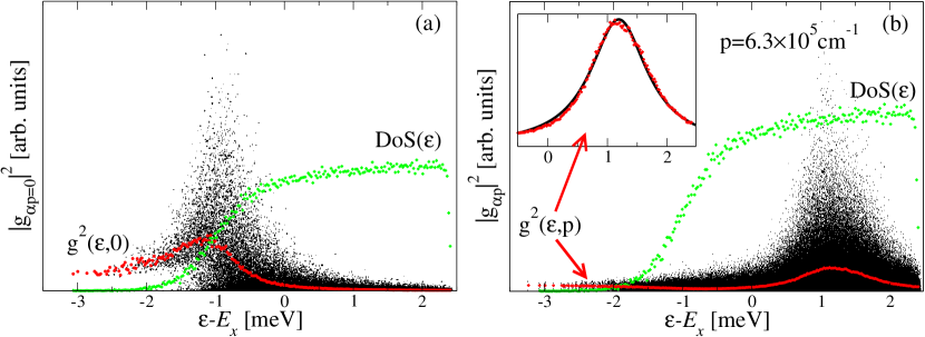
Figure 6: Distribution of energies, and energy dependence of exciton–light coupling strength, for excitons in the presence of disorder. Black points mark the energy and coupling strength of individual exciton states (combined from 160 separate disorder realisations); green lines show density of states, red lines show mean square coupling strength. Panel (a) [From [75] Copyright (2006) by the American Physical Society] coupling to zero-momentum photons. Panel (b) [From [76].] coupling to high momentum photon states (much beyond relevant states). Inset illustrates comparison of numerical values for the mean squared oscillator strength to the first Born approximation.

A relationship between the model of this section, and that of the previous section, may be established in the limit of low densities, by considering a Holstein-Primakoff transformation of the Hamiltonian in Eq. (17); i.e.

$$S_{\alpha}^{z}=D^{\dagger}_{\alpha}D_{\alpha}-\frac{1}{2},\quad S_{\alpha}^{+}=D^{\dagger}_{\alpha}\sqrt{1-D^{\dagger}_{\alpha}D^{\vphantom{\dagger}}_{\alpha}},\quad S_{\alpha}^{-}=\left(S_{\alpha}^{+}\right)^{\dagger}$$ (22)

Then, assuming the occupation of excitons to be small (i.e. $\left<D^{\dagger}_{\alpha}D_{\alpha}\right>\ll 1$), one may expand Eq. (17) to get:

$$\hat{H} = \sum_{\alpha}\varepsilon_{\alpha}D^{\dagger}_{\alpha}D_{\alpha}+\sum_{\mathbf{p}}\omega_{\mathbf{p}}\psi_{\mathbf{p}}^{\dagger}\psi_{\mathbf{p}}$$ (23)

$$+ \frac{1}{\sqrt{A}}\sum_{\alpha}\sum_{\mathbf{p}}\left(g_{\alpha,\mathbf{p}}\psi_{\mathbf{p}}D^{\dagger}_{\alpha}\left(1-\frac{1}{2}D^{\dagger}_{\alpha}D^{\vphantom{\dagger}}_{\alpha}\right)+\mathrm{H.c.}\right).$$

Comparing this to Eq. (9) shows that a bosonic model derived in this way has certain differences to the standard bosonic model; it obviously neglects the inter-exciton Coulomb term, as this was neglected in Eq. (17), and the exciton energies are set by localised states in a disorder potential $\varepsilon_{\alpha}$, rather than $\mathbf{k}^{2}/2M$. Less obviously, but more importantly, the saturation interaction term is significantly stronger than would be suggested by Eq. (9); in that case, the mean-field energy shift at polariton density $n$ is of the order of

$$\delta E^{\rm LP}_{\mathrm{sat}}\sim\Omega_{R}na_{\mathrm{ex}}^{2}.$$ (24)

In contrast, the term in Eq. (23) is of the order of

$$\delta E^{\rm LP}_{\mathrm{sat}}\sim\Omega_{R}n\xi_{d}^{2}\;$$ (25)

where $\xi_{d}\sim(MW_{\rho})^{-1/2}$ is a characteristic length scale of the disorder potential. This energy shift is important as it relates the observed lower polariton blue-shift to the polariton density, and so is important in the interpretation of experiments. This result is valid at low temperatures; at higher temperatures one can show [76], that $\xi_{d}$ should be replaced by $\xi_{T}\sim(Mk_{B}T)^{-1/2}$. The appearance of this temperature-dependent length scale would not arise from a model that included only bosonic lower polaritons. Comparison of the equilibrium transition temperatures of the two models is discussed later, in Sec. 2.4.1.

2.2.4 Comparison of models

As is clear from the above discussion, the Bose-Fermi model in some sense encompasses a bosonic model. However, its derivation led naturally to the inclusion of saturation interaction, but as yet no generalisation including long-range Coulomb interaction has been studied. The question of comparing the models is therefore not so much whether one model is right or wrong, but whether interaction effects beyond a quartic boson-boson interaction are important, and so whether a description like that of Eq. (17) is necessary. At low enough densities and temperatures (i.e. temperatures a small fraction of the Rabi splitting) it is clear such a description is not necessary. However, the definition of “low enough” that is derived from studying when the (equilibrium) phase boundary of Eq. (17) is reproduced by a bosonic theory suggests that low enough means exciton separation of the order of the wavelength of light [93, 94, 77], rather than, e.g. the exciton Bohr radius; and temperatures of the order of tenths of the Rabi splitting.

As an alternative way to resolve the question of which approximate Hamiltonian, Eq. (17) or Eq. (9), is most appropriate for a given physical system, one can propose the following clear, but technically challenging approach. From both Hamiltonians, one can construct an approximate ground state, which can then be rewritten in terms of electrons, holes and photons. In both cases, we consider generalisations of the coherent state, which for a simple structureless boson field $L^{\dagger}$ would be written $\exp(\lambda L^{\dagger})\left|0\right>$. This leads to two different trial wavefunctions for the electron-hole-photon system. While this is not a simple exercise — and would in fact require extensive numerical computation — it is a useful gedanken comparison to highlight the distinctions. Let us consider first the trial wavefunction appropriate to the Hamiltonian of Eq. (14). Taking $\left|0\right>$ as the filled valence band, we have

$$\left|\Psi_{Bose}\right>=e^{\lambda L^{\dagger}_{0}}\left|0\right>;\quad L^{\dagger}_{0}=\cos(\xi_{0})\psi^{\dagger}_{0}+\sin(\xi_{0})\sum_{\mathbf{q}}\tilde{\varphi}(\mathbf{q})c^{\dagger}_{\mathbf{q}}v_{-\mathbf{q}}.$$ (26)

At low densities this wavefunction has a simple interpretation; $\tilde{\varphi}(\mathbf{q})$ is the bound exciton wavefunction, and the $\xi_{0}$ controls the exciton and photon fractions of the lower polariton; i.e. the term in brackets is the lower polariton creation operator, and this is a coherent state of lower polaritons. Note however that $(c^{\dagger}_{\mathbf{q}}v_{-\mathbf{q}})^{2}=0$, as $c^{\dagger}_{\mathbf{q}},v_{-\mathbf{q}}$ are fermionic operators, thus this wavefunction can be also written as:

$$\left|\Psi_{Bose}\right>=\exp\left(\lambda\cos(\xi_{0})\psi^{\dagger}_{0}\right)\prod_{\mathbf{q}}\left(1+\lambda\sin(\xi_{0})\tilde{\varphi}(\mathbf{q})c^{\dagger}_{\mathbf{q}}v_{-\mathbf{q}}\right)\left|0\right>.$$ (27)

Thus, if $\tilde{\varphi}(\mathbf{q})$ has a step-like form, this can also describe a BCS-like state [95, 96]. More generally, the parameters $\lambda,\xi_{0}$ and the function $\tilde{\varphi}(\mathbf{q})$ can be taken as variational parameters, and used to minimise the energy.

Starting instead from the Hamiltonian of Eq. (17) one is instead led to write:

$$\left|\Psi_{TLS}\right> = e^{\lambda\psi^{\dagger}_{0}}\prod_{\alpha}\left(\cos(\theta_{\alpha})+\sin(\theta_{\alpha})D^{\dagger}_{\alpha}\right)\left|0\right>_{TLS}$$ (28)

$$D^{\dagger}_{\alpha} = \sum_{\mathbf{k},\mathbf{q}}\tilde{\Phi}_{\alpha}(\mathbf{k})\tilde{\varphi}(\mathbf{q})c^{\dagger}_{{m_{e}}\mathbf{k}/({m_{e}+m_{h}})+\mathbf{q}}v_{{m_{h}}\mathbf{k}/({m_{e}+m_{h}})-\mathbf{q}}$$ (29)

where we have now introduced $\tilde{\Phi}_{\alpha}(\mathbf{k})$ as the localised centre of mass wavefunction. Note that the operator, $D^{\dagger}_{\alpha}$, describing a localised exciton does not square to zero. It is thus not possible to rewrite the BCS-like product in Eq. (28) as an exponential; there is a qualitative difference between the states in Eq. (27) and Eq. (28). Although $(D^{\dagger}_{\alpha})^{2}\neq 0$, the product in Eq. (28) only allows each operator $D^{\dagger}_{\alpha}$ to occur at most once, so for a given single-particle state labelled by $\alpha$, only zero or one excitons may occupy it, and thus prevents multiple occupation. By including the disorder-localised centre of mass wavefunctions, Eq. (28) describes single occupation of a set of localised exciton wavefunctions, while in comparison, Eq. (26) describes only the single, lowest energy, delocalised exciton mode. As above, we may take the parameters $\lambda,\theta_{\alpha}$ and the functions $\tilde{\Phi}_{\alpha}(\mathbf{k}),\tilde{\varphi}(\mathbf{q})$ as variational.

Unfortunately, direct evaluation of the expectation of Eq. (3) with these trial wavefunctions is challenging. At low enough densities, no multiple occupation occurs, so in this limit Eq. (26) and Eq. (28) become comparable: Expanding Eq. (28) for small $\theta_{\alpha}$, the terms in the product can be rewritten approximately as:

$$\prod_{\alpha}\left(1+\theta_{\alpha}D_{\alpha}^{\dagger}\right)+\mathcal{O}(\theta_{\alpha}^{2})\simeq\exp\left[\sum_{\alpha}\theta_{\alpha}D_{\alpha}^{\dagger}\right]+\mathcal{O}(\theta_{\alpha}^{2}).$$ (30)

This would be equivalent to Eq. (26) except that Eq. (26) macroscopically occupies the $\mathbf{k}=0$ exciton state, whereas Eq. (30) occupies a collection of disorder-localised states. Although not identical, a superposition of many localised states distributed across the sample can (at low enough densities) behave similarly to the translationally invariant $\mathbf{k}=0$ state. Thus depending on the relative importance of disorder localisation, and on the difference of Coulomb interaction between different single-particle exciton states vs interaction for multiple occupation of the same single-particle state, one may find which of Eq. (26) or Eq. (28) has lower energy.

Furthermore, both of the above wavefunctions are mean-field approximations of the ground state, and in both cases, energy could be lowered by constructing the Nozières-Bogoliubov state. To discuss this, let us consider the simpler case of structureless bosons, $L^{\dagger}_{\mathbf{k}}$. One can then understand this state in two ways, either as a variational ansatz, as in Ref. [97]:

$$\left|\Lambda\right>=\exp\left(\lambda L^{\dagger}_{0}+\sum_{\mathbf{k}}\lambda_{\mathbf{k}}L^{\dagger}_{\mathbf{k}}L^{\dagger}_{-\mathbf{k}}\right)\left|0\right>,$$ (31)

and then find $\lambda,\lambda_{\mathbf{k}}$ by minimisation. Alternatively, the same state can be described if one considers fluctuation corrections to the mean-field theory. As is well known, in the presence of a condensate, the quasi-particles are the Bogoliubov modes [13], i.e.

$$B^{\dagger}_{\mathbf{k}}=\cosh(\phi_{\mathbf{k}})L^{\dagger}_{\mathbf{k}}+\sinh(\phi_{\mathbf{k}})L_{-\mathbf{k}},$$ (32)

with $\phi_{\mathbf{k}}$ the Bogoliubov rotation angle. Thus, given the Bogoliubov spectrum, the lowest energy state is the Bogoliubov vacuum, $\left|\Omega_{\mathrm{Bog}}\right>$, defined such that it is annihilated by all $B_{\mathbf{k}}$, i.e.

$$\left[\cosh(\phi_{\mathbf{k}})L_{\mathbf{k}}+\sinh(\phi_{\mathbf{k}})L^{\dagger}_{-\mathbf{k}}\right]\left|\Omega_{\mathrm{Bog}}\right>=0\quad\forall\mathbf{k}\;,$$ (33)

which is clearly solved by:

$$\left|\Omega_{\mathrm{Bog}}\right>=\exp\left(-\sum_{\mathbf{k}}\tanh(\phi_{\mathbf{k}})L^{\dagger}_{\mathbf{k}}L^{\dagger}_{-\mathbf{k}}\right)\left|0\right>$$ (34)

Two comments are in order about the significance of this state; firstly, the physical reason this state is of lower energy is the quartic interaction, in particular terms like $L^{\dagger}_{\mathbf{k}}L^{\dagger}_{-\mathbf{k}}L_{0}L_{0}+H.c.$, which favour states which are not eigenstates of the number of $\mathbf{k}=0$ particles. Secondly, even when projected to an overall number state, one may retain features of this state, by writing a superposition of terms with different division of the number of particles between the condensate mode and other states.

2.3 Theoretical treatments — effects of the environment

Having discussed various models of the polariton system, we now turn to how these models, and the effects of the environment, may be treated. We first briefly outline the thermal equilibrium case, and compare mean-field theories of the two models discussed above. We then discuss some of the various approaches that one may use to describe the effects of the environment, focusing mainly on non-thermal steady states. Finally, we try to separate and clarify the concepts of coherence, condensation, superfluidity and lasing, which while often related, need not necessarily occur together.

2.3.1 Thermal equilibrium

The simplest approximation for the environment is to consider the system in thermal and chemical equilibrium with a bath. While it is clear that the current experiments involve substantial pumping and decay, which will be discussed next, there are compelling reasons to deal with the equilibrium case. Firstly, the properties of a given model in the equilibrium case are instructive when considering the range of behaviour it can show; while the equilibrium properties of weakly interacting dilute Bose gas are well studied [98, 99, 13], the properties of models like Eq. (17), with distributions of oscillator strengths and energies [75, 76] are less known. Even within the weakly interacting Bose gas picture, interesting features can arise from considering non-quadratic dispersion [100, 101, 102], or the effects of anisotropic spin interactions [44, 103]. The second reason is that with improvements in the quality of mirrors, and refinement to the design of microcavities and the conditions of pumping, experiments have been able to increase the thermalisation rate to be comparable to or faster than polariton decay rates [41, 43], and so for these, or future, experiments, the correct description may become increasingly close to equilibrium.

The treatment of both Eq. (9) and Eq. (17) in equilibrium can be put in a similar form by considering their saddle point, or minimum action equations. Formally, these can be derived by writing the imaginary time path integral for the partition function [104], and then considering the configurations that minimise the imaginary time action. Thus, for the bosonic case within the effective lower polariton model, Eq. (14), the saddle point solutions satisfy a Gross-Pitaevskii equation:

$$\left[-i\partial_{t}+E^{\rm LP}_{\mathbf{k}=0}-\frac{{E^{\rm LP}_{\mathbf{k}=0}}^{\prime\prime}\nabla^{2}}{2}+\mathcal{O}(\nabla^{4})+V^{\mathrm{eff}}_{0,0,0}|L_{0}|^{2}\right]L_{0}\simeq 0$$ (35)

Here, as the dispersion $E^{\rm LP}_{\mathbf{k}}$ is not quadratic, we have expanded it to quadratic order to find the coefficient of $\nabla^{2}$. Note that by considering solutions of the form $L_{0}(t)=L_{0}e^{-i\mu t}$, one can introduce the chemical potential, and thus recover the expected static Gross-Pitaevskii equation.

For the fermionic model, more care is required; since there has been no projection onto lower polaritons, the saddle point condition leads to coupled equation for the photon field and two-level systems. Using the spin notation of Eq. (17) one has:

$$\left[-i\partial_{t}+\omega_{0}-\frac{\nabla^{2}}{2m}\right]\psi_{0}=\sum_{\alpha}\frac{g_{\alpha,0}}{\sqrt{A}}S_{\alpha}^{-}\delta(\mathbf{r}-\mathbf{r}_{\alpha});$$ (36)

$$\partial_{t}\mathbf{S}_{\alpha}=-\mathbf{B}_{\alpha}\times\mathbf{S}_{\alpha},\qquad\mathbf{B}_{\alpha}=\left(\begin{array}[]{c}g_{\alpha,0}(\psi_{0}+\psi^{\dagger}_{0})\\ g_{\alpha,0}i(\psi_{0}-\psi^{\dagger}_{0})\\ \varepsilon_{\alpha}\end{array}\right).$$ (40)

Here $\mathbf{r}_{\alpha}$ is the localisation site of the two-level system $\mathbf{S}_{\alpha}$. In the case where the only variation is $\psi_{0}(t)=\psi_{0}e^{-i\mu t}$ and the polarisation has the same time variation, one can eliminate the time variation by a gauge transformation.

The sum over exciton energy levels can also be simplified if one makes two assumptions: firstly that the excitations are occupied according to a thermal distribution, and secondly that we can average over many realisations of excitonic disorder. This second assumption, that $\psi_{0}(\mathbf{r})$ varies slowly compared to the distance between excitons, or equivalently that the photon couples to many localised exciton modes, allows one to replace the sum over exciton energy levels with a sum over the statistical distribution of energies and the excitonic coupling strengths. This then yields:

$$\left[\omega_{0}-\mu-\frac{\nabla^{2}}{2m}+\mathcal{O}(\nabla^{4})-\sum_{\alpha}\frac{g_{\alpha,0}^{2}}{A}\frac{\tanh(\beta E_{\alpha})}{2E_{\alpha}}\right]\psi_{0}\simeq 0\;,$$ (41)

where the energy $E_{\alpha}^{2}=(\varepsilon_{\alpha}-\mu)^{2}+g_{\alpha,0}^{2}|\psi_{0}(\mathbf{r})|^{2}$ depends on the local value of the slowly varying $\psi_{0}(\mathbf{r})$. Note that in this way the exciton disorder does not lead to spatial inhomogeneity of the polariton condensate, and so in the absence of photonic disorder one would expect polariton condensation in the $\mathbf{k}=0$ mode. This has a clear similarity to Eq. (35), but in this case, the non-linear interaction term is more complicated than it was in the bosonic case, $V^{\mathrm{eff}}_{0,0,0}|L_{0}|^{2}$, and the polariton-polariton interaction is due to the nonlinearity of the susceptibility arising from the saturable nature of the excitons. For a uniform and static condensed solution ($\nabla^{2}\psi_{0}=0=\partial_{t}\psi_{0}$), the Gross-Pitaevskii equation (41) is also analogous to the gap equation (self-consistency condition) of the BCS theory [104].

Despite their similarity, there is an important distinction between Eq. (35) and Eq. (41); Eq. (35) is temperature independent, while the nonlinear susceptibility in Eq. (41) decreases at high temperature, and is eventually incapable of supporting condensation. Thus one can crudely say that Eq. (35) can support mean-field condensation at any temperature, and fluctuations [98] must be considered to find a transition temperature. For the bosonic model, going beyond mean-field theory, one can also produce a temperature dependent equation by using a Hartree-Fock wavefunction, and thus including the effect of interactions between the condensate and non-condensed particles (see e.g. Ref. [13] for further details). In distinction Eq. (41) contains a finite mean-field transition temperature, and so fluctuations are only important when they significantly decrease this transition temperature [93, 77]. Thus, including fluctuations one finds a crossover from a fluctuation dominated phase boundary at low densities, to a phase boundary that is well described by mean-field theory in the high density limit, where long-range interactions dominate. The temperature dependence that appears in Eq. (41) can also be understood by noting that it was necessary to integrate out the excitonic degrees of freedom in Eq. (36) to produce an effective action for a single photon field. Thus, the saddle point density for the Bose-Fermi model contains both the condensate, and a contribution from incoherent excitons.

By considering fluctuation corrections to the saddle point density, one may in three dimensions, and at low densities, recover the non-interacting transition temperature of a weakly interacting Bose gas. i.e. considering the transition from the normal side, a mean-field condensate density appears when $\mu\to 0$, and so the critical temperature is given by $\rho_{\mathrm{total}}=\rho_{\mathrm{fluct}}(T_{c},\mu=0)$. However, for a two-dimensional system, when the transition is of the Berezhinskii-Kosterlitz-Thouless (BKT) class [105, 106, 107], it is necessary to consider fluctuations in the presence of a quasi-condensate, as the BKT transition, where free vortices proliferate, occurs below the mean-field transition temperature.

In order to calculate the total density in the presence of a condensate, it is important to note that the fluctuation corrections can deplete the condensate population, as well as increase the population of other modes [77]. The condensate density that comes from a mean-field calculation [i.e. from the uniform static solutions to Eq. (35)] is $\rho=|L_{0}|^{2}=\mu/V^{\mathrm{eff}}$. One compact way of finding how fluctuations deplete the condensate density is by using the Hugenholtz-Pines relation as discussed in e.g. Ref. [98]. Let us briefly summarise here how this argument shows that the condensate density is smaller than the mean-field estimate. To discuss this one must introduce the self energy of the condensate $\Sigma$. If we define the matrix of Green’s functions:

$$\mathcal{G}(\omega,\mathbf{k})=\int dte^{-i\omega t}\left<\left(\begin{array}[]{cc}L^{\dagger}_{\mathbf{k}}(t)L_{\mathbf{k}}(0)&L_{-\mathbf{k}}(t)L_{\mathbf{k}}(0)\\ L^{\dagger}_{\mathbf{k}}(t)L^{\dagger}_{-\mathbf{k}}(0)&L_{-\mathbf{k}}(t)L^{\dagger}_{-\mathbf{k}}(0)\end{array}\right)\right>,$$ (42)

and introduce $\mathcal{G}_{0}(\omega,\mathbf{k})$ as the free Green’s function (i.e. in the absence of interactions), then the matrix of self energies is defined by $\Sigma(\omega,k)=\mathcal{G}^{-1}_{0}(\omega,\mathbf{k})-\mathcal{G}^{-1}(\omega,\mathbf{k})$. The Hugenholtz-Pines relation is the condition required of this self energy in order that there might be a gapless mode, as one expects for a Bose-condensed system. The condition can be written as $\Sigma_{11}-\Sigma_{12}=\mu$. By writing the self energies in terms of the densities of condensate and normal state particles, one may use this identity to write the condensate density in terms of $\mu$ and the normal state density. At leading order in interaction strength, it can be shown [98] that the self energy is given by:

$$\Sigma_{11}=2V^{\mathrm{eff}}(\rho_{0}+\rho_{1}),\quad\Sigma_{12}=V^{\mathrm{eff}}(\rho_{0}-\tilde{\rho}_{1}).$$ (43)

In this expression $\rho_{0}$ is the condensate density, $\rho_{1}$ is the density of particles in other states, and $\tilde{\rho}_{1}$ is the anomalous density, $\sum_{\mathbf{k}}\langle L^{\dagger}_{\mathbf{k}}L^{\dagger}_{-\mathbf{k}}\rangle$. One thus finds: $\rho_{0}=(\mu/V^{\mathrm{eff}})-(2\rho_{1}+\tilde{\rho}_{1})$, i.e. fluctuations reduce the condensate density below its mean-field value.

To then extract the BKT temperature, one needs to find the condition for free vortices to proliferate [108, 107, 109]. As described in those works, this requires one to know the fugacity of a vortex, and the effective vortex-vortex interaction strength, both of which depend on the superfluid stiffness $\rho_{s}$, which may be found from the difference between transverse and longitudinal current response functions (see Eq. (46)). The result is a transition which occurs at $k_{B}T_{\mathrm{BKT}}=(2/\pi)(\rho_{s}/m)$. In the case of bosons with quadratic dispersion, and in the limit of weak quartic interaction strength $V^{\mathrm{eff}}$, i.e. $mV^{\mathrm{eff}}\ll 1$, one may extract an asymptotic relation between the superfluid density and the total density, giving $k_{B}T_{\mathrm{BKT}}=[2\pi/\ln(B/mV^{\mathrm{eff}})](\rho/m)$, where quantum Monte Carlo calculations [110] give $B=380\pm 3$. The phase boundary calculated according to the fermionic model, i.e. using Eq. (41), and the boundary for the BKT transition in a bosonic model following Refs. [100, 101, 102], but with the effective inclusion of disorder, are shown in Fig. 7. These boundaries are discussed further in Sec. 2.4.1.

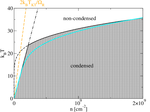
Figure 7: Phase boundaries for an equilibrium polariton condensate. Solid and dashed lines mark the mean-field phase boundary of the boson-fermion model of Refs. [75, 76] (dashed line indicates the region in which this boundary is strongly modified by fluctuation corrections). Blue lines indicate the BKT transition temperature for thermal population of the lower polariton branch, with the modified Landau criterion as discussed in Ref. [102]. The interaction strength used for this curve is that which arises from the bosonic approximation to the boson-fermion model — i.e. includes the effect of disorder in the saturation interaction. For comparison, orange dashed line marks the phase boundary for the naïve estimate (i.e. neglecting condensate depletion due to density fluctuations) BKT transition temperature for a quadratic dispersion with effective polariton mass. Plotted for $\Omega_{R}=26\mathrm{meV}$ exciton–photon detuning $\delta=\omega_{0}-\varepsilon^{\ast}=5.4\mathrm{meV}$, photon mass $m_{ph}=2.59\times 10^{-5}m_{e}$.

2.3.2 Pumping, decay, and non-equilibrium treatments

A more realistic discussion of the experimental environment must consider that polaritons may escape, and so continuous pumping is required to produce a steady state. In addition, if one is to describe pulsed experiments, or the transient behaviour after the pump is switched on, a dynamical approach is required to describe the time dependence of population [111, 112, 113, 103]. Considering for the moment steady state situations — i.e.  c.w. (continuous wave) pumping — one may highlight two important features of the difference between the pumped, decaying system and thermal equilibrium. The first is that the distribution function; i.e. the population of each energy level, may be far from thermal, and set instead by the balance of pumping, decay, and thermalisation rates; [32, 114, 115, 113, 116]. The second class of effects is that incoherent pumping and decay introduce dephasing, and can change the excitation spectrum of the system, the additional inclusion of these effects are discussed in Refs. [117, 116], (see also the discussion in Sec. 3.2.1). There are a wide variety of approaches that may be applied to study one or either of these features; in the following we discuss briefly how some of these various approaches are related, and what limitations they may have. For a more general discussion see e.g. Refs. [118, 35, 119].

In order to describe the properties of the pumped, decaying system, one requires a method to calculate various correlation functions. Given an expression for single particle correlation functions, one may then find many properties of interest, for example the occupation of modes, the luminescence and absorption spectra, and the first-order coherence properties. The most general information about one particle correlations can be written in terms of the two correlation functions $\mathcal{G}^{<}(t,\mathbf{r})=\left<\psi^{\dagger}(t,\mathbf{r})\psi(0,0)\right>$, $\mathcal{G}^{>}=\left<\psi(t,\mathbf{r})\psi^{\dagger}(0,0)\right>$, which with $\psi$ describing the photon field correspond directly to luminescence and absorption probabilities. These encode information both about the form of the spectrum and thus the density of states, and also about the population of those states. For example, the density of states is given by $\mathrm{Im}[\mathcal{G}^{R}(\omega+i0,\mathbf{k})]$, where the retarded Green’s function can be written as: $\mathcal{G}^{R}(t,\mathbf{r})=\Theta(t)[\mathcal{G}^{>}(t,\mathbf{r})-\mathcal{G}^{<}(t,\mathbf{r})]$. In equilibrium, these two Greens functions can be related in terms of the thermal distribution function, but out of equilibrium no such simplification is possible.

Let us now discuss different methods to calculate these Green’s functions. The first method is to find and solve the operator equations of motion for $\psi,\psi^{\dagger}$, and thus to evaluate the correlation functions directly. In order to describe pumping and decay, one considers coupling the system to baths, which either pump particles and energy into the system, or provide modes into which particles may decay. These baths are assumed to be large, so their properties (e.g. distribution functions) are fixed, and not affected by the system. Since the bath and system are coupled, the equations of motion for the system operators will also include bath operators. If one considers the initial state of the bath to be drawn from some fixed (e.g. thermal) distribution, then the expectation of bath operators will be random quantities, with statistical properties set by the bath’s distribution [111, 35]; thus such coupling to baths introduces noise, giving quantum Langevin equations [35]. The second method is to write equations of motion for Green’s functions, which will now involve correlation functions of bath operators, which again can be found if one assumes a fixed distribution for the baths. These coupled equations are the content of the Keldysh formalism [120], in which it turns out to be simpler to write equations for various linear combinations of the Green’s functions, allowing one to combine the Green’s functions in a compact matrix notation (see e.g. [118]). The equations for the Green’s functions can also be derived in a path integral formulation [119]. The path integral formalism allows one to make a close connection with the methods discussed in Sec. 2.3.1, and can describe changes to both the occupation and to the spectrum induced by pumping and decay [117, 116]. As such, it allows one to introduce a complex self-consistency condition (i.e. a complex equivalent of the Gross-Pitaevskii equation); this interpolates between the laser, in which self-consistency requires balancing of pumping and decay, and the equilibrium condensate, where self-consistency instead relates real self-energy shifts. This point will be discussed in more detail in Sec. 3.2.1.

The above two approaches allow one to find self-consistently the population and the spectrum in the presence of pumping and decay. In certain cases — for example in the normal state, with weak pumping and decay — the changes to the spectrum may be small, and one is interested primarily in changes to the population. By assuming a known form for the retarded Green’s function (i.e. for the spectrum of the system) it is possible to extract equations for the population from the Green’s function formalism (see Ref. [118, Chapter 9] for details). These will lead to the Boltzmann equation [121], which may also be derived phenomenologically, by considering various rates of transfer between different energies. Thus, by neglecting the “kinetic” effects, that change the spectrum, but retaining “dynamic” effects, that change the populations, one may investigate how pumping and decay change the occupation of the spectrum [32, 114, 115, 112, 113]. Even without pumping and decay, the spectrum changes due to interactions in the condensed state [13]; and further calculations retaining “kinetic” effects suggest the pumping and decay further modify the spectrum (see Refs. [117, 116] and also Ref. [122] in a different context). Because changes to the spectrum modify the density of states, they can be expected to in turn affect the population dynamics; it is therefore not clear how valid it is to consider population dynamics in the condensed system without self-consistent treatment of the changes to the spectrum.

A different approach to treating the coupling to baths is to consider the density matrix, which allows calculation of any single-time expectation of operators, as well as certain multi-time correlations, discussed further below. Calculating the full $N$-body density matrix allows calculation of correlation functions of arbitrary numbers of particles, rather than just the single particle correlations discussed above. Density matrix methods, and Green’s functions methods can be related as the single-particle density matrix (i.e. tracing over coordinates of all but one particle) is equivalent to the equal time part of the one particle Green’s function.

To numerically calculate evolution of the density matrix, due both to the system Hamiltonian, and to the effect of coupling to baths, one can choose an appropriate basis and write the density matrix in terms of a distribution function over this basis, i.e. $\hat{\rho}=\sum\left|a\right>\left<b\right|P(a,b)$. The time evolution of the density matrix then corresponds to the time evolution of this distribution function. Under certain conditions [35, 123], it is possible to interpret the evolution of this distribution as describing evolution of a quasi-probability distribution. In such a case, the equation of motion for $P(a,b)$ is a Fokker-Planck equation, and can be rewritten in terms of Langevin equations for classical variables. If one chooses to resolve the density matrix onto a basis of coherent states, a variety of ways of doing this exist, among which we mention two important choices: the positive P distribution, and the Wigner distribution (See [35] for other possible choices, and further details). The positive P distribution formally has the desired properties, and gives the desired Langevin equations, but is numerically unstable when applied to the kind of problem discussed here [123]. The Wigner distribution, although not technically matching the above requirements, can have its equation of motion approximated — the truncated Wigner representation [123, 124] — which allows one to find appropriate Langevin equations, and is numerically stable.

The Wigner distribution allows one to find the expectation of symmetrised products of operators; at equal times it is trivial to extend this to find general products of operators, by making use of equal time commutation relations. It is also possible to find multi-time correlation functions from such an approach, however since the unequal time commutation relations are not a-priori known, one cannot generally find expectations of other orders; in this sense the truncated Wigner approach does not allow $\mathcal{G}^{<}$ and $\mathcal{G}^{>}$, but only the symmetrised combination $\mathcal{G}^{<}+\mathcal{G}^{>}$, and hence cannot separate the density of states from its occupation.

2.3.3 Lasing, condensation, superfluidity

Condensation, coherence and superfluidity are often connected, however when dealing with two-dimensional systems of composite particles, where finite-size and non-equilibrium effects may be important, it is important to separate and clarify these concepts. The discussion below compares condensation, coherence and superfluidity in equilibrium infinite systems to the case including finite-size and non-equilibrium effects. For simplicity we discuss these ideas in terms of a general bosonic field $\psi^{\dagger}$, rather than any specific field appearing in the microcavity polariton system. The first concept is macroscopic occupation of single-particle wave-function; rigorously this can be defined as the existence of a macroscopic eigenvalue of the reduced one-particle density matrix [125]:

$$\rho_{1}(\mathbf{r},\mathbf{r}^{\prime})=\left<\psi^{\dagger}(\mathbf{r})\psi(\mathbf{r}^{\prime})\right>=\sum_{i}n_{i}\varphi_{i}^{\ast}(\mathbf{r})\varphi_{i}(\mathbf{r}^{\prime}),$$ (44)

where $n_{i}$ is the occupation of the single-particle mode $\varphi_{i}(\mathbf{r})$. A macroscopic eigenvalue exists if $\lim_{N\to\infty}n_{0}/N\neq 0$ where $N=\sum_{i}n_{i}$ is the total number of particles. In an infinite system, if the macroscopically occupied state is an extended state, then there is Off Diagonal Long Range Order — i.e. if in the position representation $\lim_{\mathbf{r}\to\infty}|\varphi_{0}(\mathbf{r})|\neq 0$, then there remain extensive terms far from the diagonal [126]. Thus, in such a case, the correlation function $\lim_{\mathbf{r}\to\infty}\left<\psi^{\dagger}(\mathbf{r})\psi{}(0)\right>=n_{0}\varphi_{0}^{\ast}(\mathbf{r})\varphi_{0}(0)\neq 0$. In a non-interacting two-dimensional trapped (and thus finite) gas of bosons there can be a sharp crossover to a state with a macroscopic eigenvalue (i.e. of the order of the number of particles) of the one-particle density matrix [127, 128]. However, the single-particle state $\varphi_{0}(\mathbf{r})$ to which this eigenvalue corresponds will be a state localised in the trap, and so despite the existence of a macroscopic eigenvalue, $\lim_{\mathbf{r}\to\infty}\left<\psi^{\dagger}(\mathbf{r})\psi{}(0)\right>=0$.

The visibility of interference fringes is directly related to the first-order coherence function $g_{1}(t=0;\mathbf{r})$, where:

$$g_{1}(t;\mathbf{r})=\frac{\left<\psi^{\dagger}(\mathbf{r},t)\psi(\mathbf{0},0)\right>}{\sqrt{\left<\psi^{\dagger}(\mathbf{0},0)\psi(\mathbf{0},0)\right>\left<\psi^{\dagger}(\mathbf{r},t)\psi(\mathbf{r},t)\right>}};$$ (45)

coherence can be defined by the properties of this function. As just discussed, if one defines coherence by the limit of $g_{1}(0,\mathbf{r}\to\infty)$, then in a trapped system, this function vanishes. However, coherence will exist across the size of the trap. In such inhomogeneous and complicated cases, a binary classification of coherent/incoherent is less useful than a description of how the coherence varies as a function of separation in time and space. Both the size of this variation, and its functional form will depend on the interplay of finite size (and form of trapping potential), temperature, interactions, and decay rates [116].

Superfluidity can meanwhile be defined separately as the difference of longitudinal and transverse response functions at vanishing wave-vector [129, 98, 13]:

$$\chi_{ij}(\omega=0,\mathbf{q}) = 2\int_{0}^{\beta}d\tau\left<\left<J_{i}(\mathbf{q},\tau)J_{j}(-\mathbf{q},0)\right>\right>$$ (46)

$$= \chi_{T}(q)\left(\delta_{ij}-\frac{q_{i}q_{j}}{q^{2}}\right)+\chi_{L}(q)\frac{q_{i}q_{j}}{q^{2}}\;,$$

and $\rho_{s}\propto\lim_{q\to 0}\left[\chi_{L}(q)-\chi_{T}(q)\right]$. Since superfluidity results from a change of the response functions, it occurs only in an interacting system; without interaction bosons do not become superfluid. In a two-dimensional infinite interacting system, below the BKT transition [105, 106, 107], coherence decays as a power law rather than an exponential — low energy phase fluctuations prevent true long range order [130] — and superfluidity exists, but no macroscopic occupation of a single mode.

When one considers a more realistic system, which is both interacting, but also of finite extent, one cannot ignore a-priori the physics of the BKT transition, nor can one ignore a-priori the physics of the trap. At low enough temperatures it is clear there will be macroscopic occupation of a single mode, and full coherence across the trap. How this state is approached as temperature is reduced, or as density is increased differs depending on whether interactions or finite size effects are dominant. If described as a non-interacting gas, the coherence at all distances increases uniformly as a single mode is increasingly occupied [127, 128]. In the BKT scenario, power law correlations develop on intermediate scales (between some short range thermal length and the trap size); then as temperature decreases, the thermal length increases and the power with which correlations decay decreases, again restoring full coherence as $T\to 0$ [131, 132], as shown in Fig. 8.

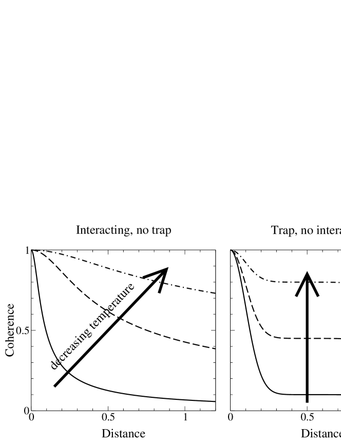
Figure 8: Sketches of the spatial decay of coherence, $g_{1}(t=0;\mathbf{r})$. Left: interacting infinite 2D Bose gas, showing power-law decay at long distances. Right: non-interacting trapped gas; at short distances (less than the thermal length) perfect coherence exists; on intermediate lengthscales coherence reaches a constant value, due to the non-zero condensate fraction; coherence eventually goes to zero for separations larger than the trap size.

Adding non-equilibrium effects, the nature of decay of correlations in an infinite system is significantly altered [117, 116]. The long wavelength phase modes, responsible for decay of correlations become diffusive. i.e. the poles of the Green’s functions, which in the equilibrium case have the form $\omega\simeq\pm ck$, take instead the form $\omega\simeq ix\pm\sqrt{(ck)^{2}-x^{2}}$ in the pumped and decaying case. This is illustrated in Fig. 9.

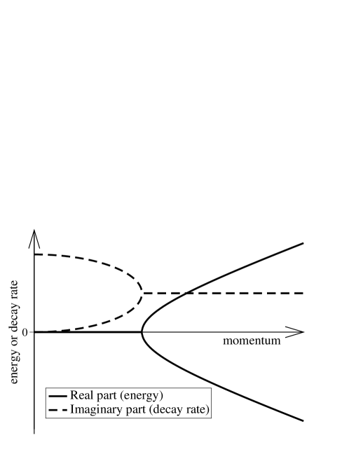
Figure 9: Sketch of momentum dependence of real and imaginary parts of poles of the Green’s function, in the presence of pumping and decay. At zero momentum, there is a free phase, i.e. a mode with vanishing real and imaginary part. For small momentum both modes are diffusive, with no real part, but a non-zero imaginary part. Only above some critical momentum does a real part develop. Such results are seen both in the calculations in Refs. [117, 116], and also for resonant pumping (as discussed in Sec. 3.2.1) in Refs. [122, 133].

Combining the effects of phase diffusion, and discrete level spacing [116] the properties of coherence are further modified, and one approaches the laser limit: temporal coherence of laser emission comes from one, or at most a few modes (resonant with the laser cavity), and so phase diffusion of a single mode [14] leads always to exponential decay of temporal correlations [134, 135, 136]. As well as this distinction of forms of temporal coherence, it is worth mentioning here a few other important distinctions between lasing and the generalised concept of condensation discussed here, as there are evidently also similarities [137]. Most obviously, polariton condensation is seen at the polariton resonance, which is significantly (of the order of the Rabi splitting $\Omega_{R}$) below the lowest cavity photon mode; as such nonlinear emission coexisting with strong coupling is a signal that one should consider polaritons, and not just photon lasing. A more fundamental difference is that lasing requires inversion, while condensation does not; this is a consequence of the standard laser systems possessing little coherence in the gain medium, while excitons, being part of a coherent polaritons, are coherent [138, 139, 140, 141, 142]. This distinction can also be seen by comparing the critical lasing condition to the Gross-Pitaevskii equations of Eq. (35) and Eq. (41). In the presence of pumping and decay, the susceptibility (describing the nonlinear response of excitons) becomes complex [117, 116]; the real part of the susceptibility gives the nonlinearity in the Gross-Pitaevskii equation. In contrast, the imaginary part of the susceptibility describes absorption or gain, and leads to the lasing condition, that round trip gain and loss balance. A treatment of a model system with pumping and decay elegantly shows how these conditions can be combined, giving an expression in terms of the total susceptibility [117, 116].

Starting from the strong-coupling regime, when crossing over to the weak-coupling regime (see, e.g. [143, 25, 144]), the polariton splitting collapses, and so the lasing mode no longer has any excitonic character, and becomes the standard photon laser. A major advantage of an exciton-polariton laser over standard lasers is that it can operate without the inversion of the electronic population [145], and therefore it has a much smaller threshold pump power. It is interesting to note that wide band gap semiconductors, such as GaN and ZnO, would be particularly suitable as in these cases excitons are stable at higher temperatures and densities, and therefore they could operate at room temperature. Electronic population inversion is not necessary because in the exciton-polariton laser, both photon field and excitons are coherent. In addition, the involvement of the excitonic field leads to strong nonlinear effects compared to conventional lasers, due to exciton-exciton interactions.

2.4 Phenomena

The previous two sections discussed the models, and the treatments of the environment, that have been used to theoretically model polariton condensates. This section in contrast will review a few of the phenomena that have been predicted as possible signatures and properties of a polariton condensate.

2.4.1 $T_{c}$ and the phase boundary

Within a given model, and effective description of the environment, it is natural to first ask under what conditions a condensate can exist. Within an equilibrium model of the lower polariton branch as weakly interacting bosons, phase diagrams for the physical parameters of various possible materials are shown in Refs. [100, 101] (however, see Ref. [102] for a discussion of the effects of non-quadratic dispersion on the BKT transition temperature). By considering a simplified version of the Bose-Fermi model Eq. (18), where the energies $\varepsilon_{\alpha}$ are described by a Gaussian distribution, while all excitons display a fixed coupling to light, the mean-field phase boundary was first calculated in Refs. [86, 87]. The effect of fluctuations, restoring the bosonic limit at low densities was instead considered in Refs. [93, 77]. Since the content of the boson-fermion model at small densities and temperatures is equivalent to a bosonic model, and the low momentum part of the polariton dispersion is controlled by the photon mass, it is not surprising that it is possible to recover the standard BKT transition temperature of a weakly interacting Bose gas from the boson-fermion model in the low density limit. A calculation of the mean-field boundary which instead takes into account a realistic description of the quantum well disorder and the full distribution of oscillator strengths (see Fig. 6) has been performed in Refs. [75, 76] (see Fig. 7).

Owing to finite size effects the experimental systems do not have a sharp phase transition marking the onset of a broken symmetry. All the observed transitions are rounded, and in order to extract a phase boundary from experiment, some criterion has to be chosen. One commonly used criterion is the nonlinear threshold; i.e. the point at which the relation between emission at $\mathbf{k}=0$ and input pump power becomes nonlinear. Such a criterion is somewhat problematic. A second-order phase transition can be expected to be accompanied by a region with large susceptibilities, and thus such nonlinearity extends over a significant range of parameters, and so identification of a strict phase boundary from it is hard. Only in a mean-field theory does the onset of nonlinearity occur at the transition. However, because of the long-range nature of interactions, mean-field theory can be an adequate description for lasers, and for polariton condensates except at very low densities (as can be seen from Fig. 7). The following sections discuss other phenomena that may demonstrate or describe condensation and coherence in microcavity polariton systems, and may thus provide alternative, or corroborating experimental criteria to find the phase boundary.

2.4.2 Energy-resolved luminescence, resonant Rayleigh scattering

In both the weakly interacting boson model, and the Bose-Fermi model, condensation leads to changes in the spectrum of polariton modes — most significantly the appearance of the phase modes [98, 13]. In addition, for a model starting from localised exciton states, with a distribution of energies and oscillator strengths, there is weak emission from sub-radiant exciton states between the upper and lower polaritons [146]. This emission is also modified by condensation [75]: in the presence of a condensate these sub-radiant exciton states have energies $E_{\alpha}$ as defined following Eq. (41), and so the density of states is changed by the coupling to the coherent field. This change to the emission is discussed further in detail Ref. [76]. In practice, it is however hard to observe the incoherent luminescence of thermally excited modes in the presence of a strong signal from the coherent condensate. One suggestion to overcome this problem is to probe these excited modes via resonant Rayleigh scattering; by using a phase sensitive measurement one may be able to identify a small coherent scattering signal even in the presence of emission from the condensate [75, 76]. Fig. 10 shows the Rayleigh scattering signal expected both above and below the phase transition; note in the condensed case, one sees linear modes both above and below the chemical potential; this is as one expects from the Bogoliubov spectrum, where the normal modes are superpositions of particle creation and annihilation.

Figure 10: Contourplot of the disorder averaged RRS intensity $\left<I_{\mathbf{p}\mathbf{q}}(\omega)\right>$ for $|\mathbf{p}|=|\mathbf{q}|$ as a function of the dimensionless momentum $|\mathbf{p}|a_{\mathrm{ex}}$ and rescaled energy $2(\omega-\mu)/\Omega_{\mathrm{R}}$, for zero detuning, Rabi splitting $\Omega_{\mathrm{R}}=26$meV, temperature $k_{B}T=20$K, and a disorder strength characterised by an inverse scattering time $1/\tau=1.16$meV. (a) non-condensed (density $\rho\simeq 0$); (b) condensed regime ($\rho\simeq 3.6\times 10^{9}\mbox{cm}^{-2}$) ; (c) condensed regime ($\rho\simeq 3.1\times 10^{10}\mbox{cm}^{-2}$) . Green lines mark chemical potential: if non-condensed RRS emission is present only above the chemical potential, but when condensed, it is present both above and below. [From [76]].

2.4.3 Momentum distribution of radiation

By integrating the luminescence at a given wave-vector, one may consider the momentum distribution of polaritons — this has also been discussed in the context of exciton condensation [132, 147]. In a weakly interacting, two-dimensional, infinite system, the density of states would be constant, and this would just show the Bose-Einstein distribution. In experiments, the distribution at small momentum is close to, but can deviate from the Bose-Einstein distribution [36, 41]. However, such deviations are expected; both due to interactions, which modify the spectrum and so modify the density of states [93, 77], and also due to finite size, which cuts off components at small wave-vectors. A naive calculation shows how the change of spectrum causes a change of density of states: for a weakly interacting Bose gas with dispersion $\varepsilon_{\mathbf{k}}$, and mean-field equation $\mu=g\rho_{0}$, we have the Bogoliubov spectrum $E_{\mathbf{k}}=\pm\sqrt{\varepsilon_{\mathbf{k}}(\varepsilon_{\mathbf{k}}+2g\rho_{0})}$, and simple algebra gives the density of states:

$$\nu_{s}(\omega,\mathbf{k}) = \mathrm{Im}\left[\mathcal{G}^{R}(\omega+i0^{+},\mathbf{k})\right]=\mathrm{Im}\left[\frac{i\omega+\varepsilon_{\mathbf{k}}+g\rho_{0}}{\omega^{2}+E_{\mathbf{k}}^{2}}\right]$$ (47)

$$= \frac{E_{\mathbf{k}}+\varepsilon_{\mathbf{k}}+g\rho_{0}}{2E_{\mathbf{k}}}\delta(\omega-E_{\mathbf{k}})+\frac{E_{\mathbf{k}}-\varepsilon_{\mathbf{k}}-g\rho_{0}}{2E_{\mathbf{k}}}\delta(\omega+E_{\mathbf{k}})\;.$$

This suggests that as $\mathbf{k}\to 0$, the density of states goes like $g\rho_{0}/E_{\mathbf{k}}\propto 1/k$, however this neglects the fact that the low energy modes are phase modes, and phase fluctuations may grow without bounds, as only their gradient costs energy; a full calculation, e.g. [141, 77], shows that this term becomes $1/k^{2-\eta}$ with $\eta\simeq 2T/T_{BKT}$. In order to include the effects of finite size, one approach is to start with the zero-temperature Thomas-Fermi spatial profile, for which coherence across the whole cloud leads to sharp angular peaks, and then consider how phase fluctuations destroy the long range coherence, and thus soften the peaks [132]. There have also been calculations of this momentum distribution for non-equilibrium situations, where details of the dynamics of polariton relaxation lead to a maximum of the distribution at non-zero $\mathbf{k}$, e.g. Refs. [32, 115, 113, 112].

2.4.4 Linewidth, first- and second-order coherence, polarisation

The line-shape of emission is controlled by the Fourier transform of the first-order coherence function as a function of time, i.e. $g_{1}(t;\mathbf{r}=0)$, using $g_{1}(t;\mathbf{r})$ defined in Eq. (45). A perfectly coherent single mode source would have $g_{1}(t;0)$ constant, and thus infinitely sharp lines. Although at any finite temperature, population of slow phase modes will lead to some decay of $g_{1}(t;0)$, the transition to a condensed phase will lead to a slower decay of $g_{1}(t;0)$, as has been seen [49]. Similarly, as discussed in Sec. 2.3.3, one can also consider the spatial decay of coherence [41]; which has also been much studied in cold atomic gases (see, theoretical discussion in Refs. [148, 131, 149] and experiments in Refs. [150, 151, 152]).

The calculation of coherence has already been discussed briefly in Sec. 2.3.3. As was stressed there, a distinction exists between coherence of a few mode laser [134], applied to the polariton problem in Refs. [135, 136]; and coherence in a continuum of modes [111, 117, 116]. In both cases increasing temporal coherence in the system should lead to a narrowing of linewidth as the phase transition is approached, however the behaviour far above the transition may differ. This is clear from the fact that for a single mode with a quartic interaction, the equilibrium state is a number state, and so starting from a coherent state, one has phase diffusion due to self phase modulation even in the absence of any pumping or decay [136]. For a many-mode system, the ground state is neither a coherent nor a number state, and is better described by the Bogoliubov-Nozières state [97], thus it is not clear that the same effect — i.e. self phase modulation causing larger broadening — should persist.

A related measurement is the second-order coherence function (see e.g. Ref. [35]):

$$g_{2}(t)=\frac{\left<\psi^{\dagger}(\mathbf{r},0)\psi^{\dagger}(\mathbf{r},t)\psi(\mathbf{r},t)\psi(\mathbf{r},0)\right>}{\left<\psi^{\dagger}(\mathbf{r},0)\psi(\mathbf{r},0)\right>\left<\psi^{\dagger}(\mathbf{r},t)\psi(\mathbf{r},t)\right>}$$ (48)

As mentioned above, for a thermal state, $g_{2}(t=0)=2$, while for a coherent state $g_{2}(t=0)=1$. Experimental measurement of $g_{2}(t=0)$ is restricted by finite detector integration times, and since $g_{2}(t)=1$ at times when $g_{1}(t;0)\to 0$, it is hard to distinguish the value of $g_{2}(t=0)$ [33, 49]. The dynamical behaviour of $g_{2}(t=0)$ as a function of time following switching on the pump laser [153, 154, 155], or from an equilibrium picture with separate coherent and incoherent contributions [44] has been considered. Within the Bose-Fermi model, the second-order coherence has been studied for a finite number of excitons coupled to a single coherent field, where the finite number of states replaces the phase transition with a smooth crossover [156].

Considering the differences of interaction strength between polaritons with parallel and anti-parallel spin polarisations, Laussy et al. [44] have shown that condensation should be associated with spontaneous development of a linear polarisation. That a condensate should choose some definite polarisation state is a much more general result, i.e. that repulsive interactions prevent fragmentation of a condensate, even when there are two single-particle states with identical energies [96]. Considering the specific form of the interaction, Laussy et al. showed that this specific polarisation should be a linear state (as opposed to circular or elliptical). Note, however, that the pinning of the polarisation to one of the crystallographic axes observed in Refs. [41, 45, 46] cannot be an effect of spontaneous symmetry breaking, but it is instead likely due to some optical anisotropy of the microcavities. In atomic gases, investigation of “spinor condensates” is hard, as it requires the use of all optical trapping, as a magnetic field would Zeeman split the atomic spin states; further the populations of spin species are effectively fixed at the start of the experiment, so rather than polarisation, phase separation into spin domains has been observed there [157].

3 Resonant pumping

Since its first realisation in 2000 [158], the possibility of reaching the stimulated scattering regime for polaritons by resonant pumping has attracted considerable interest [159, 160, 161, 162, 31, 163, 164, 165, 166, 167, 168, 169, 170], and has initiated the search for polariton lasers and a new generation of ultrafast optical amplifiers and switches. In resonant excitation experiments, polaritons are optically pumped at an energy and momentum which allows coherent polariton-polariton scattering directly into the ground state. In pulsed, ultrafast pump-probe experiments, a second pump is used to initiate the stimulated scattering process to the ground state, while for c.w. (continuous wave) excitation the stimulated regime can be self-induced above some pump threshold. As in non-resonant excitation experiments, the direct mapping between in-plane momentum and angle of bulk photons is crucial. It is this direct mapping that allows one to directly pump at a given momentum, and thus to perform the experiments described here.

The macroscopic occupation of the ground state in these experiments differs in some ways from condensation and spontaneous coherence arising from incoherent pumping. In experiments without a probe pulse, there is a free phase between the pump and signal modes, however as discussed in Sec. 3.2.1, the existence of a free phase alone is not sufficient to ensure superfluidity in such driven systems. Further, since the coherence of the signal beam is directly coupled to the pump beam, higher order correlations, and the linewidth of the signal may be inherited from the pump. Experiments with an additional probe beam at the signal frequency differ yet further; in such experiments the phase of the signal is fixed by the probe, and so in this case all excitations ought to be gapped.

It is interesting to note that the idea of parametric scattering discussed here for polaritons has been recently applied in a different field; that of dilute gases of atoms confined in an optical lattice [171, 172]. We will discuss this example in more detail later in Sec. 4.1.

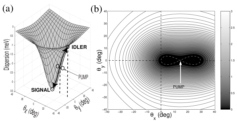
Figure 11: (a) Lower polariton dispersion; (b) countorplot of $|E^{\rm LP}_{\mathbf{k}}+E^{\rm LP}_{2\mathbf{k}_{p}-\mathbf{k}}-2E^{\rm LP}_{\mathbf{k}_{p}}|$ as a function of $\mathbf{k}$ and the zero value contour (white dashed). A pair of final states (signal and idler) can be found by intersecting the white dashed curve with a straight line passing through $\mathbf{k}_{p}$ (indicated as pump). [From [173] Copyright (2001) by the American Physical Society].

3.1 Summary of experiments

The main idea of resonant pumping experiments [158, 159, 160, 161, 162, 31, 163, 164, 165, 166, 167, 168, 169, 170] is that of the coherent scattering of two polaritons from the resonantly pumped mode (pump) into the ground state (signal) and a high energy state (idler) [see Fig. 11(a)]. Energy and momentum conservation in this scattering requires one to have $\{\mathbf{k}_{p},\mathbf{k}_{p}\}\mapsto\{0,2\mathbf{k}_{p}\}$, where

$$E^{\rm LP}_{\mathbf{k}=0}+E^{\rm LP}_{2\mathbf{k}_{p}}=2E^{\rm LP}_{\mathbf{k}_{p}}\;,$$ (49)

which uniquely selects the momentum (i.e. angle) of pump, signal and idler. If one instead relaxes the condition $\mathbf{k}=0$ for the signal mode, then for a fixed pump angle $\mathbf{k}_{p}$, it can be shown [173, 168] that those final states which satisfy energy and momentum conservation describe a figure-of-eight in momentum space [see Fig. 11(b)]. The non-parabolic dispersion of polaritons is crucial in order to obtain such a resonant scattering processes, and so the analogous process for excitons is forbidden. Resonant experiments can be divided into two types: In the first type the scattering is stimulated by a weak probe field (parametric amplification), while in the second type there is no probe and the seed to initiate stimulation is provided by the pump itself, if above a certain power threshold (parametric oscillation).

In their pioneering work [158], Savvidis and collaborators realised the stimulated scattering regime for the first time in an InGaAs/GaAs/AlGaAs microcavity with a Rabi splitting of $\Omega_{R}=7$meV. By pumping polaritons at the “magic” angle $\theta\simeq 17^{\circ}$ (for zero exciton–photon detuning) close to the inflection point of the LP dispersion curve, and using a second pump at zero angle (probe) to initiate the process, a substantial gain of up to 70 was observed. The large observed signal required both the “magic” angle pumping, and the probe at zero angle, and was absent either if no probe was applied [159] (see Fig. 12), or when pumping at different angles even in presence of the zero angle probe. These results provide strong evidence for a polariton scattering process stimulated by the probe. The bosonic scattering rate is enhanced by a factor $N+1$ where $N$ is the population of bosons in the final state [174], in this case the ground state. Moreover, stimulated scattering was confirmed in this experiment by the observed exponential dependence of the gain on pump power. Note however that the obtained stimulated regime is more correctly described as a ‘parametric’ amplifier rather than a laser, i.e. the population of the lowest mode is amplified by a phase coherent parametric process [163].

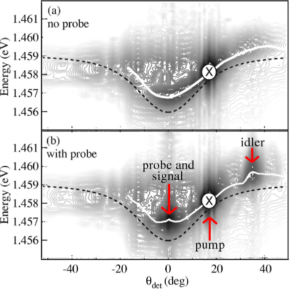
Figure 12: Contour maps of the PL emission spectra for excitation at the ‘magic’ angle ($\times$) (a) when no probe is applied at zero angle and (b) when a probe is applied, which stimulates a strong gain in the probe direction. The peak of the PL (white line) shows a marked asymmetry and a blue-shift of $\sim 0.7$meV with respect to the low power polariton dispersion (dashed). [From [159] Copyright (2000) by the American Physical Society].

Much experimental work has followed this first result [159, 160, 161, 162, 31, 163, 164, 165, 166, 167, 168, 169, 170]. Evidence of stimulated scattering has been obtained in [31], with a three beam pulsed experiment, where two pumps excite states at large and opposite angles, $\theta_{p}\sim\pm 45^{\circ}$, and a third beam is used as a probe at normal incidence. Here, the pump creates a quasi-thermal exciton reservoir at large momentum; then, scattering of polariton from $\mathbf{k}_{p}$ and $-\mathbf{k}_{p}$ to the $\mathbf{k}=0$ upper and lower polariton states can occur, and is is stimulated by the occupation (due to the probe) of the final state. Note that, at zero detuning, such a scattering process conserves energy ($2\varepsilon^{\rm ex}_{\mathbf{k}}=E^{\rm LP}_{0}+E^{\rm UP}_{0}$) and momentum. Recent experiments in the original two beam pump probe configuration, but with time resolved measurements as a function of different pump and probe angles have begun the investigation of the hydrodynamic properties of the injected “polariton fluid” [175, 176].

In another series of experiments, making use of resonant c.w. excitation [162, 160] rather than ultrafast pulsed excitation as in [158, 159, 31], the stimulated scattering regime has been reached even without the probe beam (parametric oscillation). Here, the stimulated scattering is self-initiated when the pump power is strong enough that the final state population becomes close to one. It is interesting to note that, as in the non-resonant excitation experiments, a minimum pump power is required (with threshold-like behaviour) in order to overcome the ‘bottleneck’ effect and thus provide the occupation of the ground state required to stimulate scattering. In these particular experiments, occupation of the ground state was estimated to be close to $1$ at threshold and around $300$ at the highest pump powers. A maximum blue-shift of the lower polariton of the order of $0.5$meV was observed, which is much less than the Rabi splitting of $\sim 6$meV, and so confirms that the experiment is always in the strong coupling regime. Because of the stimulated scattering, pumping of the ground state mode is efficient, and so these systems have a low power threshold, typically $5$ times smaller than for a high quality vertical cavity surfaces emitting laser (VCSEL) [160].

While the experiments described above were at temperatures of the order of $5$K, Saba and collaborators have reported pump-probe parametric amplification of polaritons with an extraordinary gain up to $5000$ at temperatures up to $120$K in GaAlAs-based microcavities, and up to $220$K in CdTe-based microcavities [164]. The highest possible operating temperatures for observing amplification have been shown to be determined by the exciton binding energy ($25$meV for the used CdTe wells and $13.5$meV for GaAs wells), rather than the polariton Rabi splitting, which in these experiments varies from $25$meV for the 24 quantum-well (QW) CdTe microcavity to $15$meV and $20$meV for GaAlAs microcavities with respectively 12 QWs and 36QWs. Time-resolved measurements, obtained by controlling the delay between pump and probe, show ultrafast dynamics of the parametric gain, promising future applications in high-repetition-rate optical switches and amplifiers.

As an alternative to the finite angle resonant configuration, a few experiments [163, 169] have concentrated on the double energy and momentum resonance, where pump, signal and idler are all at normal incidence, $\mathbf{k}_{p}=0$. In this geometry it is possible to investigate the dependence of the phase of the signal on the phase of the pump, and thus to show [163] that in this degenerate configuration the parametric scattering is a coherent process. In addition, in most of the early resonant experiments, such as Refs. [159, 160, 162, 164], spectral narrowing of the signal was observed when amplification occurs, also suggesting that the signal is coherent [166]. Direct evidence for the coherent nature of the signal emission has come only recently, in Ref. [170], where first-order temporal and spatial coherence were investigated. In that work, in a resonant c.w. pump, no probe, configuration, two spots separated by $70\mu$m, coming from the same laser excited region of the sample ($100\mu$m FWHM of Gaussian profile), are overlapped in momentum space, showing interference fringes. In addition, by making use of noise measurements, the emitted signal is shown to be in a single-mode quantum state, rather than in a multi-mode state.

Recently, the pair correlation of the emitted signal-idler polaritons have been demonstrated by showing that polaritons in two distinct idler modes can interfere if and only if they share the same signal mode [177].

3.2 Theories

Predictions about threshold conditions, spectral properties and efficiency of the amplification in resonant pump-probe experiments can be easily obtained by making use of the effective lower polariton Hamiltonian $H_{\rm LP}$ (14) described in Sec. 2.2.2, to which one must add the coupling to the external radiation pump $\Omega_{\rm pump}(t)$ and probe $\Omega_{\rm probe}(t)$ fields [178]:

$$H_{\rm ext}=c\sum_{\mathbf{k}}\left\{\left[\delta_{\mathbf{k},\mathbf{k}_{p}}\Omega_{\rm pump}(t)+\delta_{\mathbf{k},0}\Omega_{\rm probe}(t)\right]\cos\theta_{\mathbf{k}}L_{\mathbf{k}}^{\dagger}+\rm{H.c.}\right\}\;.$$ (50)

A closed set of equations of motion for the expectation values of probe (signal) $\left<L_{0}(t)\right>$, pump $\left<L_{\mathbf{k}_{p}}(t)\right>$, and idler $\left<L_{2\mathbf{k}_{p}}(t)\right>$ modes can be obtained by factorising field expectation values, and neglecting higher order correlations. By solving such equations, both in the steady-state regime and numerically for the pulsed excitation, Ciuti and collaborators [178] have obtained the conditions for gain threshold, showing that the efficiency of the amplifier depends very strongly on the polariton linewidth; the larger the linewidth, the higher the threshold and the lower the maximum gain. Similar results, such as the blue-shift of the signal with increasing pump power, have been obtained by Whittaker [179] in a classical nonlinear optics treatment. In Whittaker’s paper, a phenomenological model — where a nonlinear excitonic oscillator is coupled to the cavity mode, driven by external fields — can describe both parametric amplification and oscillation. This treatment, considering classical fields, and retaining only the frequencies corresponding to pump, signal and idler modes, is equivalent to factorising the field expectation values and considering the equation of motion for $\left<L_{0}(t)\right>$, $\left<L_{\mathbf{k}_{p}}(t)\right>$, and $\left<L_{2\mathbf{k}_{p}}(t)\right>$.

By considering the case of a c.w. pump without a probe, and expanding up to the second-order in the field expectation values, it can be also shown [173, 18] that, below threshold for parametric amplification, the polariton photoluminescence,

$${\rm PL}(\mathbf{k},t,\omega)\simeq\cos^{2}\theta_{\mathbf{k}}\Re\int_{0}^{\infty}d\tau e^{-i(\omega-i0^{+})\tau}\left<L_{\mathbf{k}}^{\dagger}(t+\tau)L_{\mathbf{k}}(t)\right>\;,$$ (51)

has a blue-shifted asymmetric emission distribution, as was observed in [159], and shown in Fig. 12. The lower polariton blue-shift here, $E^{\rm LP}_{\mathbf{k}}\mapsto E^{\rm LP}_{\mathbf{k}}+V^{\rm eff}_{\mathbf{k},\mathbf{k}_{p},0}\left<L_{\mathbf{k}_{p}}\right>^{2}$, is due to the interaction term of Eq. (16). Note that the above formalism is valid only below the threshold for parametric emission, as above threshold the equation of motion for the pump mode, describing pump depletion should also be included.

Recent theoretical work [180], including the effects of polariton blue-shifts on the parametric oscillator equations, has shown that in the c.w. configuration the ‘magic’ angle is not necessary, as it is in the ultrafast pump-probe case, and that, under suitable pump conditions, the parametric oscillator can in general be observed for pump angles $\theta\gtrsim 10^{\circ}$. Such calculations seem to explain the experimental results obtained in Ref. [167]. In that experiment, with c.w. pumping, stimulation was achieved over a wide range of pump angles, from $10^{\circ}$ to $24^{\circ}$ and with the signal always at $\mathbf{k}=0$. Including the polariton blue-shift also allows one to distinguish parametric oscillation, where output intensity grows continuously, and bistability, where output suddenly jumps at some threshold pump power, and shows hysteresis if power is then reduced. The regimes of bistability and parametric oscillation have been investigated as a function of pump angle for resonant pumping [180], and also allowing for mismatch between pumping frequency and the polariton energy at the pumping angle [181].

There has also been a proposal to study the hydrodynamic properties of the injected polariton fluid by studying its coherent scattering by disorder [182]; i.e. resonant Rayleigh scattering. In the proposed experiment, a strong pump beam creates a large coherent population of polaritons, and also provides the source of polaritons which may be coherently scattered: In the presence of disorder, the polaritons can resonantly scatter to states with different momentum, but the same energy. This can be observed by looking at the angular distribution of photons escaping the cavity which are resonant with the pump beam. At low pump power, this emission pattern will be a ring, at the pump angle — i.e. those states with the same energy have the same modulus of momentum. However, since a large coherent population of polaritons modifies the polariton dispersion relation, at higher pump powers, both the shape and intensity variation across the pattern of resonantly scattered photons reveal information about the polaritons in the cavity.

3.2.1 Phase degree of freedom and low energy modes

The laser and an equilibrium polariton condensate form extreme ends of the spectrum of systems in which coherent emission results from a symmetry breaking transition; the resonantly pumped polariton laser falls somewhere in between. Although, as discussed in Sec. 3.1, the coherence of the signal is inherited from the pump, in the parametric oscillator configuration, without a seed signal beam there is in principle a free phase $\Delta\phi$ between the signal and pump modes. That is, the equations of motion are invariant under the transformation $\hat{L}_{0}\to\hat{L}_{0}e^{i\Delta\phi}$, $\hat{L}_{2\mathbf{k}_{p}}\to\hat{L}_{2\mathbf{k}_{p}}e^{-i\Delta\phi}$, using the notation introduced on page 50. In an equilibrium condensate, the invariance of the energy under a global rotation of phase implies the existence of a soft phase mode. However, the existence of a free phase does not necessarily lead to the same consequences [122, 117, 133, 116], as we will discuss next.

Amongst several distinctions between a laser and an equilibrium condensate, one important difference is that for a laser, the threshold condition is the balance of gain and decay [14, 137, 174], while for a condensate, the Gross-Pitaevskii equation (gap equation, self-consistency condition) involves the real parts of the self-energy. This difference implies a difference in the spectrum of fluctuations. Both cases have a pole in the fluctuation spectrum at $\omega=0$ and zero wavevector, corresponding to global phase rotations. However, for small, but non-zero wavevector, the spectrum first acquires a real part for a true condensate, describing linearly dispersing modes [129, 98] (in an interacting system); if instead one must balance gain and decay, the spectrum instead first acquires an imaginary part, describing diffusive modes [122, 117, 133, 116] (see Fig. 9). Although both the laser and strongly pumped polariton systems share this diffusive structure, there is an important difference in the properties of the phase mode between a conventional laser and the strongly-pumped polariton system. The difference is that, as discussed in Sec. 2.3.3, a conventional laser has a discrete spectrum of wavevectors (all other modes rapidly decay), while the microcavity polariton system has a continuum of in-plane wavevectors with comparable decay rates. The continuum of diffusive phase modes should thus lead to differences between the coherence properties of a laser and a resonantly pumped polariton system [122, 133]. The difference between diffusive and dispersive low energy degrees of freedom may also have implications for pattern formation in nonlinear systems [183, 184].

3.2.2 Polarisation and spin relaxation

By considering the spin of polaritons, with resonant pumping, one can consider the coupled dynamics of the polarisations of the pump, signal and idler modes. This dynamics leads to a rich variety of physical effects, due to the interplay between spin dependent stimulated scattering, and precession induced both by momentum dependent TE-TM (Transverse-Electric, Transverse-Magnetic) splitting, and other energy splittings due to polariton-polariton interactions. The following is a brief summary of the theories that have been applied to explain these features. Interest in the subject began with experiments, in both c.w. [185] and pulsed [186] experiments, that could not be explained by regarding each spin species as acting independently. In Ref. [185], signal intensity as a function of pump ellipticity (from linear to circular) was studied, and a maximum found at an intermediate value. In Ref. [186], a large output signal was seen for a linearly polarised pump, but a circularly polarised probe, and was explained there in terms of stimulated spin scattering. In addition, the direction of the linear component of polarisation of the signal was observed to vary as a function of the degree of ellipticity of the pump beam. This large rotation was discussed in Ref. [187] as a giant Faraday effect, with the cavity amplifying the effect of spin splitting of the exciton energy levels, with the spin splitting being due to unequal spin populations of the exciton states. In contrast, Ref. [188] showed that parts of the above results could be explained by introducing coupling between the two circular polarisations. Such coupling provides two new terms; parametric scattering of cross polarisations, and processes where pump and signal, or pump and idler polaritons exchange polarisation. These terms lead to a threshold power that depends on ellipticity of the pump, and can under some conditions show lowest threshold for an elliptic polarisation.

In a different experiment, Martín et al. [189] investigated the dependence of the circular polarisation of the non-linear emission on the detuning between the cavity photon modes and excitons. This result, showing oscillations of the polarisation, have been attributed to the dependence of the TE-TM splitting on the detuning [190]. This TE-TM splitting, which depends on wave-vector, can lead to time-dependent oscillations of the polarisation of the signal and idler modes, as discussed in [191]. In order to combine the precession due to such a splitting with a spin-dependent stimulated scattering to the signal state, one is led to write a spin dependent Boltzmann equation [191]. This formalism was sufficient to reproduce the results of the experiment described in Ref. [192]. In that experiment the circular polarisation component of the signal was studied as a function of pumping strength, for both linear and circular polarisation. It was found that, for a linear pump, there is a maximum of the degree of circular signal polarisation near the nonlinear threshold. As discussed in Ref. [192], this effect can be understood as a competition between two effects; self-induced Larmor precession, which rotates the pseudospin describing the polarisation from linear to circular polarisation, and stimulated scattering to the ground state: Far above threshold, the rate of scattering to the ground state is too high to allow time for any change of polarisation in the pump mode.

An ingredient missing from the works listed so far was stimulated scattering due to polariton-polariton interactions (as opposed to polariton-phonon scattering, stimulated by final state polariton population). Shelykh et al. considered the dominant, parallel spin, interaction in Ref. [193]. However it was later realised [194, 195] that the scattering of anti-parallel spin states, though small, is important, as it leads (at high densities) to a $90^{\circ}$ rotation of linear polarisation direction between pump and signal. In a recent experiment [67], the polarisation of the output signal was studied for a linearly polarised pump, as a function of pump power and angle of the linear polarisation. This experiment showed that, just above threshold, the signal was elliptical, with the major axis (the direction of the linear component) rotated with respect to the linear polarisation of the pump — i.e. the direction of major axis depended on the direction of polarisation of the pump, but the angle between the two directions was not constant. In addition, the degree of linear polarisation of the signal decreased far above threshold (as well as the degree of circular polarisation as observed in Ref. [192]). This rotation was reproduced in a model combining precession due to static and self-induced (Larmor) splittings (including an extra in-plane splitting, as discussed in Ref. [67]) as well as spin rotation in stimulated polariton-polariton scattering. The reduction of linear polarisation far above threshold was explained by rapid self-induced Larmor precession, which rotates the linear polarisation direction so rapidly that it averages to zero.

4 Connection to other systems, conclusions

4.1 Atomic gases and Feshbach resonances

Microcavity polaritons and their condensation are related to the physics of two-component atomic Fermi gases near Feshbach resonances. In particular, the crossover from a fluctuation dominated phase boundary to a mean-field phase boundary with increasing polariton density is closely related to the BEC-BCS crossover recently studied in these atomic gases [196, 197]. For atomic gases, in contrast to polariton experiments, the density of particles is typically kept fixed, while the interaction strength is varied via magnetically tunable Feshbach resonances, allowing one to go from a BEC of bound molecules to a BCS state of fermionic pairs. The interaction strength is tuned by changing the detuning between the zero of energy for pairs of atoms in their original spin states, and a closed channel resonance level of atoms in some higher energy spin configuration (See Ref [198] and Refs therein for more details).

The Bose-Fermi model used for polaritons and described in section 2.2.3 is very similar to the model initially proposed for the description of the BEC-BCS crossover in atomic Fermi gases [199]. The fermionic operators $b^{\dagger},a^{\dagger}$ in the polariton model, introduced in Eq. (18), are analogous to the two spin species of atoms in the Feshbach resonance model; the photon is analogous to the closed channel resonance level; the dipole interaction relates to the hyperfine interaction; and the polariton to the Feshbach molecule. There are, however, a number of important differences between the two models; most notably the absence of a direct four-fermion interaction in the polariton model, and the existence of an energy dependence, and a distribution, of exciton-photon coupling strengths. Secondly there is a marked difference of mass ratios: For polaritons, the photon mass is typically a factor of $10^{5}$ times smaller than the exciton mass; in the Feshbach case the closed channel resonance has a dispersion controlled by a mass which is twice the atomic mass. Note also that there is a difference in interpretation between the photon and the closed channel resonance level in Feshbach resonance. Although inside the microcavity a photon is not an eigenstate — the upper and lower polaritons are instead eigenstates — outside the cavity it is possible to physically separate the photons from excitons. Similarly, the closed channel resonance level is not an eigenstate; however, in distinction from the photon, it cannot be physically separated from the other two-body states to which it is coupled: In general one cannot have a given molecular resonance level in isolation from other molecular states. Another difference between the systems comes in how the gap equation [i.e. Eq. (41)], and constraint on the density can be used to find chemical potential and temperature: In the mean-field (BCS) limit of the atomic case, the closed channel resonance level lies at high energies, the chemical potential lies well within the band of fermionic states, and so the density depends only on chemical potential, and not on temperature. In the polariton model, the chemical potential remains below the bottom of the band of fermionic states, and so both temperature and chemical potential influence the density. Rather, the fluctuation dominated (BEC) to mean-field (BCS) crossover of the polariton model is in the nature of which excitations are responsible for depopulating the condensate at finite temperatures.

Another issue worth considering is that further analysis has questioned the need to use the Bose-Fermi model in applications to experimentally relevant Feshbach resonances. It has been shown [200, 201] that the molecules created in the vicinity of a Feshbach resonance are halo dimers extending over large distances in which the closed channel admixture is tiny. Thus, the resonance level acts to enhance the effective interaction between fermionic pairs, but the crossover to loosely bound molecules does not rely on the macroscopic occupation of this level (as was initially suggested). Since the resonance level is not significantly occupied, it was shown, by using realistic atomic potentials [202], that the BCS-BEC crossover in atomic Fermi gases near Feshbach resonances is of the same nature as originally considered by Leggett [203]. That is, it is based on the smooth crossover of the pair size and not on the macroscopic occupation of the resonance level. Thus, microcavity polariton experiments in the normal operating conditions of large photon field occupation present the first experimental realisation of the BEC-BCS crossover which differs substantially from the original scenario [203, 93, 77].

Finally, it is interesting to note that the same idea of parametric scattering and amplification in a resonant pumping configuration as is described in Sec. 3, has been recently applied to an ultracold dilute gas of bosonic atoms confined in an optical lattice [172] (see also the related experiments on dynamic instabilities [204, 205], and four wave mixing of matter waves [171]). There, a ⁸⁷Rb Bose-Einstein condensate was loaded into a moving one-dimensional optical lattice. The optical lattice causes the atomic dispersion to deviate from quadratic, and allows parametric scattering: Atom pairs with initial momentum $k_{p}$ inherited from the moving lattice scatter elastically into two final states; $k_{p}-k$ and $k_{p}+k$. By generating a seed of atoms with momentum $k_{p}-k$, parametric amplification of both the seed and the conjugate momentum has been observed, with a gain determined by the atomic scattering length.

4.2 Excitons, quantum hall bilayers, triplons

The high quantum degeneracy temperatures and the high degree of control obtained by laser photo-excitation suggest that excitonic systems should also provide excellent environments in which to study macroscopic coherence phenomena. Much interest over the last two decades has been attracted by excitons in bulk Cu₂O crystals (see, e.g.,Ref. [206] and references therein). Excitons in Cu₂O have a large binding energy ($\sim 150$meV) and the fact that the direct dipole transition from the exciton ground state is forbidden guarantees low radiative recombination rates. In Cu₂O crystals however non-radiative recombination processes such as the Auger effect cause loss and heating, and represent the main obstacle to the observation of quantum degeneracy in these structures.

Low radiative recombination rates together with high cooling rates can be obtained for spatially indirect excitons in coupled quantum wells. Here, an electric field is applied along the growth direction, in such a way that electrons and holes separate into different wells. In contrast to the case of direct excitons, lifetimes up to few microseconds can be achieved, while the high cooling rate gives a much shorter thermalisation time, typically in the nanosecond range. As a consequence, in coupled quantum well structures, thermal equilibrium with the lattice can be relatively easily obtained by either waiting a few nanoseconds after photo-excitation or allowing the excitons to travel away from the excitation spot. While much experimental work has been done on these structures in the last few years[207, 208, 209, 210] (for review see [211, 212]), unambiguous evidence for Bose-Einstein condensation of indirect excitons in coupled quantum wells is still missing and is the subject of intensive on-going studies. Recently, gases of indirect excitons have been trapped and equilibrated using in-plane potentials, either by applying localised stress to change the local band energies [213] or by means of optical [214] or electrostatic [215] traps. The confinement of indirect excitons prevents the fast reduction of initial density which occurs in the absence of trapping due to fast expansion driven by their strong dipole-dipole repulsive interaction and their relatively high mobility.

It is interesting to note that, for an untrapped system, while the formation of an external excitonic ring has been explained as an in-plane charge separation, at low temperatures it has been shown that, such a ring can separate into a periodic array of beads, and that the light emitted by each of these beads is coherent [216]. The origin of such a phenomenon is still unknown.

Recently, experimental evidence suggests that, under appropriate conditions, an electron-electron semiconductor bilayer system in the Quantum Hall regime can condense into a superfluid state which might be interpreted as an excitonic-like superfluid [217]. In a bilayer 2D electron system with total filling factor $\nu_{T}=1$, excitonic pairs can be thought of as formed by filled electron states in one layer and empty electron states in the second layer. By changing the ratio between intra- and inter-layer Coulomb interactions, signatures of the transition to a condensed excitonic phase have been shown by a dramatic increase in the tunnelling rate between the two layers at zero interlayer voltage [218], in Coulomb drag measurements [219], and in counterflow measurements [220].

Another condensed matter system in which a phase transition can be described as condensation of an excitonic mode is that of magnetic “triplon” excitations. This has been seen in a variety of compounds including TlCuCl₃ [221, 222], BaCuSi₂O₆ [223] and Pb₂V₃0 [224], where by changing the applied magnetic field, there is a crossing between spin singlet and spin triplet excitations. The resultant magnetic phase transition can be described as condensation of the triplet magnon mode. Very recently such a transition was seen at room temperature, using parametric laser pumping to create a non-equilibrium density of triplons in the compound Y₃Fe₂(FeO₄)₃ [225].

4.3 Conclusions

In this article we reviewed the experimental results to date demonstrating coherence in microcavities, and discussed the variety of theoretical models and techniques that have been used to describe it. We discussed experiments with both non-resonant pumping, in which coherence may spontaneously arise from an initially incoherent source of polaritons, and the optical parametric amplifier and optical parametric oscillator: Both kinds of experiments allow one to explore the interplay of strong-coupling, coherence, lasing and condensation. In our discussion of theoretical descriptions, we highlighted those aspects of these solid state systems which can introduce new questions about coherence — disorder, decoherence, particle flux, potentially non-thermal distributions.

Of course, there are subjects connected to coherence in microcavities that we have not had space to discuss, or have only discussed briefly. For example, we have only briefly mentioned here questions about the dynamics of condensate formation, and of the polariton response following short pump pulses. The last years have seen rapid experimental progress in this field, with the first convincing evidence of coherence developing from incoherently injected polaritons in a variety of systems [41, 47, 58]. This experimental progress both gives hope for the possibility of future experiments, and applications on coherent microcavity polaritons, as well as focusing attention on those areas in which further theoretical work is necessary. There are areas in which our discussion has been brief because some questions have only been partially addressed to date: Questions about hydrodynamics in such partially coherent, pumped decaying systems. In order to address questions about the generic behaviour of such systems, it is important to understand how the variety of models used to describe polaritons relate, and what features each can explain. Finally, let us mention that there remains an interesting topic which can be the subject of much future research: what new experiments are possible in these light-matter systems that were not possible in either lasers or in atomic gases.

References

References

- [1] Björk G, Machida S, Yamamoto Y and Igeta K 1991 Phys. Rev. A 44 669
- [2] Weisbuch C, Nishioka M, Ishikawa A and Arakawa Y 1992 Phys. Rev. Lett. 69 3314
- [3] Ramon G, Mizrahi U, Akopian N, Braitbart S, Gershoni D, Reinecke T L, Gerardot B D and Petroff P M 2006 Phys. Rev. B 73 205330
- [4] Yoshi T, Schere A, Hendrickson J, Khitrova G, Gibbs H M, Rupper G, Ell C, Shchekin O B and Deppe D G 2004 Nature 432 200
- [5] Badolato A, Hennessy K, Atatüre M, Dreiser J, Hu E, Petroff P M and Imamoglu A 2005 Science 308 1158
- [6] Reithmaler J P, Sȩk G, Löffer A, Hoffmann C, Kuhn S, Reitzenstein S, Keldysh L, Kulakovskii V D, Reinecke T L and Forchel A 2004 Nature 432 197
- [7] Dasbach G, Diederichs C, Tignon J, Ciuti C, Roussignol P, Delalande C, Bayer M and Forchel A 2005 Phys. Rev. B 71 161308
- [8] Kaitouni R I et al. 2006 Phys. Rev. B 74 155311
- [9] Daïf O E, Baas A, Guillet T, Brantut J P, Kaitouni R I, Morier-Genoud F and Deveaud B 2006 Appl. Phys. Lett. 88 061105
- [10] Baas A et al. 2006 Phys. Stat. Sol.(b) 243 2311
- [11] Langbein W and Hvam J M 2002 Phys. Rev. Lett. 88 047401
- [12] Leggett A J 2001 Rev. Mod. Phys. 73 307
- [13] Pitaevskii L P and Stringari S 2003 Bose-Einstein Condensation (Clarendon Press, Oxford)
- [14] Haken 1970 In Kay and Maitland, eds., Quantum Optics (Academic Press, London). p. 201
- [15] Skolnick M S, Fisher T A and M W D 1998 Semicond. Sci. Technol. 13 645
- [16] Savona V, Piermarocchi C, Quattropani A, Schwendimann P and Tassone F 1999 Phase Transitions 68 169
- [17] Khitrova G, Gibbs H M, Jahnke F, Kira M and Koch S W 1999 Rev. Mod. Phys. 71 1591
- [18] Ciuti C, Schwendimann P and Quattropani A 2003 Semicond. Sci. Technol. 18 S279
- [19] Yamamoto Y, Tassone F and Cao H 2000 Semiconductor Cavity Quantum Electrodynamics, vol. 167 of Springer Tracts in Modern Physics (Springer-Verlag, Berlin)
- [20] Kavokin A and Malpuech G 2003 Cavity Polaritons, vol. 32 of Thin Films and Nanostructures (Elsevier, NY)
- [21] Baumberg J J and Viña L, eds. 2003 Special Issue on Microcavities, vol. 18 of Semiconductor Science and Technology
- [22] Deveaud B, ed. 2005 Special Issue: Physics of Semiconductor Microcavities, vol. 242 of Physica Status Solidi (b), p. 2147
- [23] Yamamoto Y and İmamoğlu A 1999 Mesoscopic Quantum Optics (Wiley, New York)
- [24] Pau S, Cao H, Jacobson J, Björk G, Yamamoto Y and Imamoğlu A 1996 Phys. Rev. A 54 R1789
- [25] Cao H, Pau S, Jacobson J M, Björk G, Yamamoto Y and Imamoğlu A 1997 Phys. Rev. A 55 4632
- [26] Dang L S, Heger D, André R, Bœuf F and Romestain R 1998 Phys. Rev. Lett. 81 3920
- [27] Boeuf F, André R, Romestain R, Si Dang L, Péronne E, Lampin J F, Hulin D and Alexandrou A 2000 Phys. Rev. B 62 R2279
- [28] Alexandrou A, Bianchi G, Péronne E, Hallé B, Boeuf F, André R, Romestain R and Si Dang L 2001 Phys. Rev. B 64 233318
- [29] Senellart P and Bloch J 1999 Phys. Rev. Lett. 82 1233
- [30] Senellart P, Bloch J, Sermage B and Marzin J Y 2000 Phys. Rev. B 62 R16263
- [31] Huang R, Tassone F and Yamamoto Y 2000 Phys. Rev. B 61 R7854
- [32] Tassone F, Piermarocchi C, Savona V, Quattropani A and Schwendimann P 1997 Phys. Rev. B 56 7554
- [33] Deng H, Weihs G, Santori C, Bloch J and Yamamoto Y 2002 Science 298 199
- [34] Weihs G, Deng H, Huang R, Sugita M, Tassone F and Yamamoto Y 2003 Semicond. Sci. and Technol. 18 S386
- [35] Gardiner C W and Zoller P 2004 Quantum Noise (Springer-Verlag, Berlin), 3rd edn.
- [36] Deng H, Weihs G, Snoke D, Bloch J and Yamamoto Y 2003 P.N.A.S. 100 15318
- [37] Weihs G, Deng H, Snoke D and Yamamoto Y 2004 Phys. Stat. Sol. (a) 201 625
- [38] Bloch J, Sermage B, Perrin M, Senellart P, André R and Dang L S 2005 Phys. Rev. B 71 155311
- [39] Bloch J, Sermage B, Jacquot C, Senellart P and Thierry-Mieg V 2002 Physica E 13 390
- [40] Richard M, Kasprzak J, Romestain R, André R and Dang L S 2005 Phys. Rev. Lett. 94 187401
- [41] Kasprzak J et al. 2006 Nature 443 409
- [42] Richard M, Kasprzak J, André R, Romestain R, Dang L S, Malpuech G and Kavokin A 2005 Phys. Rev. B 72 201301
- [43] Deng H, Press D, Götzinger S, Solomon G S, Hey R, Ploog K H and Yamamoto Y 2006 Phys. Rev. Lett. 97 146402
- [44] Laussy F P, Shelykh I A, Malpuech G and Kavokin A 2006 Phys. Rev. B 73 035315
- [45] Klopotowski L, Martín M, Amo A, Viña L, Shelykh I, Glazov M, Malpuech G, Kavokin A and André R 2006 Solid State Communications 139 511
- [46] Amo A, Martín M D, Ballarini D, Viña L, Sanvitto D, Skolnick M S and Roberts J S 2005 2 3868
- [47] Snoke D W 2006. private communication
- [48] Balili R B, Snoke D W, Pfeiffer L and West K 2006 Appl. Phys. Lett. 88 031110
- [49] Kasprzak J 2006 Condensation of Exciton Polaritons. Ph.D. thesis, Universite Joseph Fourier, Grenoble
- [50] Sellers I R, Semond F, Leroux M, Massies J, Disseix P, Henneghien A L, Leymarie J and Vasson A 2006 Phys. Rev. B 73 033304
- [51] Sellers I R et al. 2006 Phys. Rev. B 74 193308
- [52] Savvidis P G, Connolly L G, Skolnick M S, Lidzey D G and Baumberg J J 2006 Phys. Rev. B 74 113312
- [53] Butte R, Christmann G, Feltin E, Carlin J F, Mosca M, Ilegems M and Grandjean N 2006 Phys. Rev. B 73 033315
- [54] Christmann G, Butte R, Feltin E, Carlin J F and Grandjean N 2006 Phys. Rev. B 73 153305
- [55] Tawara T, Gotoh H, Akasaka T, Kobayashi N and Saitoh T 2004 Phys. Rev. Lett. 92 256402
- [56] Lidzey D G, Bradley D D C, Virgili T, Armitage A, Skolnick M S and Walker S 1999 Phys. Rev. Lett. 82 3316
- [57] Lidzey D G, Bradley D D C, Skolnick M S, Virgili T, Walker S and Whittaker D M 1998 Nature 395 53
- [58] Baumberg J J 2006. private communication
- [59] Haug H and Koch S W 2004 Quantum Theory of the Optical and Electronic Properties of Semiconductors (World Scientific, Singapore), 4th edn.
- [60] Zimmermann R 1992 Phys. Stat. Sol. (b) 173 129
- [61] Runge E 2002 Excitons in Semiconductor Nanostructures, vol. 57 of Solid State Physics (Academic Press, New York)
- [62] Gurioli M, Bogani F, Cavigli L, Gibbs H, Khitrova G and Wiersma D S 2005 Phys. Rev. Lett. 94 183901
- [63] Whittaker D M 1998 Phys. Rev. Lett. 80 4791
- [64] Starace A F 1971 Phys. Rev. A 3 1242
- [65] Kobe D H 1979 Phys. Rev. A 19 205
- [66] Cohen-Tannoudji C, Dupont-Roc J and Grynberg G 1989 Photons and Atoms (Wiley, New York)
- [67] Krizhanovskii D N, Sanvitto D, Shelykh I A, Glazov M M, Malpuech G, Solnyshkov D D, Kavokin A, Ceccarelli S, Skolnick M S and Roberts J S 2006 Phys. Rev. B 73 073303
- [68] Usui T 1959 Progr. Theor. Phys. 23 787
- [69] Hanamura E and Haug H 1977 Phys. Rep. 33 209
- [70] Rochat G, Ciuti C, Savona V, Permarocchi C, Quattropani A and Schwendimann P 2000 Phys. Rev. B 61 13856
- [71] Ciuti C, Savona V, Piermarocchi C, Quattropani A and Schwendimann P 1998 Phys. Rev. B 58 7926
- [72] Shumway J and Ceperley D M 2001 Phys. Rev. B 63 165209
- [73] Fernández-Rossier J, Tejedor C, Muñoz L and Viña L 1996 Phys. Rev. B 54 11582
- [74] Ben-Tabou de Leon S and Laikhtman B 2001 Phys. Rev. B 63 125306
- [75] Marchetti F M, Keeling J, Szymańska M H and Littlewood P B 2006 Phys. Rev. Lett. 96 066405
- [76] Marchetti F M, Keeling J, Szymańska M H and Littlewood P B 2006 cond-mat/0608096
- [77] Keeling J, Eastham P R, Szymanska M H and Littlewood P B 2005 Phys. Rev. B 72 115320
- [78] Abrahams E, Anderson P W, Licciardello D C and Ramakrishnan T V 1979 Phys. Rev. Lett. 42 673
- [79] Lee P A and Ramakrishnan T V 1985 Rev. Mod. Phys. 57 287
- [80] Lifshitz I M 1964 Adv. Phys. 13 483
- [81] Halperin B I and Lax M 1966 Phys. Rev. 148 722
- [82] Zittartz J and Langer J S 1966 Phys. Rev. 148 741
- [83] Runge E and Zimmermann R 1998 In B Kramer, ed., Advances in Solid State Physics (Vieweg, Braunschweig), vol. 38. pp. 251–263
- [84] Runge E and Zimmermann R 2000 Phys. Stat. Sol. (b) 221 269
- [85] Dicke R H 1954 Phys. Rev. 93 99
- [86] Eastham P R and Littlewood P B 2000 Solid State Commun. 116 357
- [87] Eastham P R and Littlewood P B 2001 Phys. Rev. B 64 235101
- [88] Hepp K and Lieb E 1973 Ann. Phys 76 360
- [89] Hepp K and Lieb E 1973 Phys. Rev. A 8 2517
- [90] Wang Y K and Hioe F T 1973 Phys. Rev. A 7 831
- [91] Rza̧żewski K, Wódkiewicz K and Żakowicz W 1975 Phys. Rev. Lett 35 432
- [92] Popov V and Fedotov S 1988 Sov. Phys. JETP 67 535
- [93] Keeling J, Eastham P R, Szymanska M H and Littlewood P B 2004 Phys. Rev. Lett. 93 226403
- [94] Littlewood P B, Eastham P R, Keeling J M J, Marchetti F M, Simons B D and Szymanska M H 2004 J. Phys.: Condens. Matter 16 S3597
- [95] Nozières P and Schmitt-Rink S 1985 J. LTP 59 195
- [96] Nozières P 1995 In Griffin et al. [99], p. 15
- [97] Nozières P and Saint James D 1982 J. Physique 43 1133
- [98] Popov V N 1983 Functional Integrals in Quantum Field Theory and Statistical Physics (D. Reidel, Dordrecht)
- [99] Griffin A, Snoke D and Stringari S, eds. 1995 Bose-Einstein Condensation (Cambridge University Press, Cambridge)
- [100] Kavokin A, Malpuech G and Laussy F P 2003 Phys. Lett. A 306 187
- [101] Malpuech G, Rubo Y G, Laussy F P, Bigenwald P and Kavokin A V 2003 Semicond. Sci. Technol. 18 S395
- [102] Keeling J 2006 Phys. Rev. B 74 155325
- [103] Rubo Y G, Kavokin A V and Shelykh I A 2006 Phys. Lett. A 358 227
- [104] Nagaosa N 1999 Quantum Field Theory in Condensed Matter Physics (Springer-Verlag, Berlin)
- [105] Nelson D R and Kosterlitz J M 1977 Phys. Rev. Lett. 39 1201
- [106] Kosterlitz J M and Thouless D J 1973 J. Phys. C: Solid State Phys. 6 1181
- [107] Fisher D and Hohenberg P 1988 Phys. Rev. B 37 4936
- [108] Nelson D R 1983 In C Domb and J Lebowitz, eds., Phase Transitions and Critical Phenomena (Academic Press, London), vol. 7, chap. 1. p. 2
- [109] Stoof H T C and Bijlsma M 1993 Phys. Rev. E 47 939
- [110] Prokof’ev N, Ruebenacker O and Svistunov B 2001 Phys. Rev. Lett. 87 270402
- [111] Mieck B and Haug H 2002 Phys. Rev. B 66 075111
- [112] Cao H T, Doan T D, Tran Thoai D B and Haug H 2004 Phys. Rev. B 69 245325
- [113] Doan T D, Cao H T, Tran Thoai D B and Haug H 2005 Phys. Rev. B 72 085301
- [114] Tassone F and Yamamoto Y 1999 Phys. Rev. B 59 10830
- [115] Porras D, Ciuti C, Baumberg J J and Tejedor C 2002 Phys. Rev. B 66 085304
- [116] Szymańska M H, Keeling J and Littlewood P B 2006 cond-mat/0611456
- [117] Szymańska M H, Keeling J and Littlewood P B 2006 Phys. Rev. Lett. 96 230602
- [118] Kadanoff L and Baym G 1962 Quantum Statistical Mechanics (W. A. Benjamin, New York)
- [119] Kamenev A 2005 In H Bouchiat, Y Gefen, S Guéron, G Montambaux and J Dalibard, eds., Nanophysics: Coherence and transport (Elsevier, Amsterdam), vol. LXXXI of Les Houches, p. 177
- [120] Keldysh L V 1965 Sov. Phys. JETP 20 1018
- [121] Lifshitz E M and Pitaevskii L P 1999 Physical Kinetics (Butterworth-Heinemann, Oxford)
- [122] Wouters M and Carusotto I 2005 Phys. Rev. B 74 245316
- [123] Steel M J, Olsen M K, Plimak L I, Drummond P D, Tan S M, Collett M J, Walls D F and Graham R 1998 Phys. Rev. A 58 4824
- [124] Carusotto I and Ciuti C 2005 Phys. Rev. B 72 125335
- [125] Penrose O and Onsager L 1956 Phys. Rev. 104 576
- [126] Yang C N 1962 Rev. Mod. Phys. 34 694
- [127] Bagnato V and Kleppner D 1991 Phys. Rev. A 44 7439
- [128] Ketterle W and van Druten N J 1996 Phys. Rev. Lett. 54 656
- [129] Khalatnikov 2000 An Introduction to the Theory of Superfluidity (Westview Press, Boulder)
- [130] Mermin N D and Wagner H 1966 Phys. Rev. Lett. 17 1133
- [131] Petrov D S, Holzmann M and Shlyapnikov G V 2000 Phys. Rev. Lett. 84 2551
- [132] Keeling J, Levitov L S and Littlewood P B 2004 Phys. Rev. Lett. 92 176402
- [133] Wouters M and Carusotto I 2006 cond-mat/0606755
- [134] Holland M, Burnett K, Gardiner C, Cirac J I and Zoller P 1996 Phys. Rev. A 54 R1757
- [135] Tassone F and Yamamoto Y 2000 Phys. Rev. A 62 063809
- [136] Porras D and Tejedor C 2003 Phys. Rev. B 67 161310
- [137] Haken H 1975 Rev. Mod. Phys. 47 67
- [138] Szymanska M H and Littlewood P B 2002 Solid State Commun. 124 103
- [139] Szymanska M H, Littlewood P B and Simons B D 2003 Phys. Rev. A 68 013818
- [140] Eastham P R, Szymanska M H and Littlewood P B 2003 Solid State Commun. 127 117
- [141] Marchetti F M, Simons B D and Littlewood P B 2004 Phys. Rev. B 70 155327
- [142] Marchetti F M, Szymanska M H, Eastham P R, Simons B D and Littlewood P B 2004 Solid State Commun. 134 111
- [143] Houdré R, Gibernon J L, Pellandini P, Stanley R P, Oesterle U, Weisbuch C, O’Gorman J, Roycroft B and Ilegems M 1995 Phys. Rev. B 52 7810
- [144] Butté R, Delalleau G, Tartakovskii A I, Skolnick M S, Astratov V N, Baumberg J J, Malpuech G, Di Carlo A, Kavokin A V and Roberts J S 2002 Phys. Rev. B 65 205310
- [145] Imamoğlu A, Ram R J, Pau S and Yamamoto Y 1996 Phys. Rev. A 53 4250
- [146] Houdré R, Stanley R P and Ilegms M 1996 Phys. Rev. A 53 2711
- [147] Zimmermann R 2006 Phys. Stat. Sol. (b) 243 2358
- [148] Naraschewski M and Glauber R J 1999 Phys. Rev. A 59 4595
- [149] Polkovnikov A, Altman E and Demler E 2006 PNAS 103 6125
- [150] Hagley E W et al. 1999 Phys. Rev. Lett. 83 3112
- [151] Bloch I, Hänsch T W and Esslinger T 1999 Nature 403 166
- [152] Hadzibabic Z, Kruger P, Cheneau M, Battelier B and Dalibard J 2006 Nature 441 1118
- [153] Rubo Y G, Laussy F P, Malpuech G, Kavokin A and Bigenwald P 2003 Phys. Rev. Lett. 91 156403
- [154] Rubo Y G 2004 Phys. Stat. Sol. (a) 201 641
- [155] Laussy F P, Malpuech G, Kavokin A and Bigenwald P 2004 Phys. Rev. Lett. 93 016402
- [156] Eastham P R and Littlewood P B 2006 Phys. Rev. B 73 085306
- [157] Stenger J, Inouye S, Stamper-Kurn D M, Miesner H J, Chikkatur A P and Ketterle W 1998 Nature 396 345
- [158] Savvidis P G, Baumberg J J, Stevenson R M, Skolnick M S, Whittaker D M and Roberts J S 2000 Phys. Rev. Lett. 84 1547
- [159] Savvidis P G, Baumberg J J, Stevenson R M, Skolnick M S, Whittaker D M and Roberts J S 2000 Phys. Rev. B 62 R13278
- [160] Baumberg J J, Savvidis P G, Stevenson R M, Tartakovskii A I, Skolnick M S, Whittaker D M and Roberts J S 2000 Phys. Rev. B 62 R16247
- [161] Houdré R, Weisbuch C, Stanley R P, Oesterle U and Ilegems M 2000 Phys. Rev. Lett. 85 2793
- [162] Stevenson R M, Astratov V N, Skolnick M S, Whittaker D M, Emam-Ismail M, Tartakovskii A I, Savvidis P G, Baumberg J J and Roberts J S 2000 Phys. Rev. Lett. 85 3680
- [163] Messin G, Karr J P, Baas A, Khitrova G, Houdré R, Stanley R P, Oesterle U and Giacobino E 2001 Phys. Rev. Lett. 87 127403
- [164] Saba M et al. 2001 Nature 414 731
- [165] Huynh A, Tignon J, Larsson O, Roussignol P, Delalande C, André R, Romestain R and Dang L S 2003 Phys. Rev. Lett. 90 106401
- [166] Kundermann S, Saba M, Ciuti C, Guillet T, Oesterle U, Staehli J L and Deveaud B 2003 Phys. Rev. Lett. 91 107402
- [167] Butte R, Skolnick M S, Whittaker D M, Bajoni D and Roberts J S 2003 Phys. Rev. B 68 115325
- [168] Langbein W 2004 Phys. Rev. B 70 205301
- [169] Diederichs C, Tignon J, Dasbach G, Ciuti C, Lamaitre A, Bloch J, Roussignol P and Delalande C 2006 Nature 440 904
- [170] Baas A, Karr J P, Romanelli M, Bramati A and Giacobino E 2006 Phys. Rev. Lett. 96 176401
- [171] Deng L, Hagley E W, Wen J, Trippenbach M, Band Y, Julienne P S, Simsarian J E, Helmerson K, Rolston S L and Phillips W D 1999 Nature 398 218
- [172] Campbell G K, Mun J, Boyd M, Streed E W, Ketterle W and Pritchard D E 2006 Phys. Rev. Lett. 96 020406
- [173] Ciuti C, Schwendimann P and Quattropani A 2001 Phys. Rev. B 63 041303
- [174] Scully M O and Zubairy M S 1997 Quantum Optics (Cambridge University Press)
- [175] Baumberg J J and Lagoudakis P G 2005 Phys. Stat. Sol. (b) 242 2210
- [176] Lagoudakis P G and Baumberg J J 2006. Private communication
- [177] Savasta S, Stefano O D, Savona V and Langbein W 2005 Phys. Rev. Lett. 94 246401
- [178] Ciuti C, Schwendimann P, Deveaud B and Quattropani A 2000 Phys. Rev. B 62 R4825
- [179] Whittaker D M 2001 Phys. Rev. B 63 193305
- [180] Whittaker D M 2005 Phys. Rev. B 71 115301
- [181] Wouters M and Carusotto I 2006 cond-mat/0607719
- [182] Carusotto I and Ciuti C 2004 Phys. Rev. Lett. 93 166401
- [183] Staliunas K 2001 Int. J. Bifurc. Chaos 11 2845. patt-sol/9912004
- [184] Denz C, Schawb M and Weilnau C 2003 Transverse-Patern Formation in Photorefractive Optics, vol. 188 of Springer Tracts in Modern Physics (Springer-Verlag, Berlin)
- [185] Tartakovskii A I, Krizhanovskii D N and Kulakovskii V D 2000 Phys. Rev. B 62 R13298
- [186] Lagoudakis P G, Savvidis P G, Baumberg J J, Whittaker D M, Eastham P R, Sklonick M S and Roberts J S 2002 Phys. Rev. B 65 161310(R)
- [187] Kavokin A, Lagoudakis P, Malpuech G and Baumberg J J 2003 Phys. Rev. B 67 195321
- [188] Eastham P R and Whittaker D M 2003 Phys. Rev. B 68 075324
- [189] Martín M D, Aichmayr G, Viña L and André R 2002 Phys. Rev. Lett. 89 077402
- [190] Panzarini G, Andreani L C, Armitage A, Baxter D, Skolnick M S, Astratov V N, Roberts J S, Kavokin A V, Vladimirova M R and Kaliteevski M A 1999 Phys. Rev. B 59 5082
- [191] Kavokin K V, Shelykh I A, Kavokin A V, Malpuech G and Bigenwald P 2004 Phys. Rev. Lett. 92 017401
- [192] Shelykh I, Kavokin K V, Kavokin A V, Malpuech G, Bigenwald P, Deng H, Weihs G and Yamamoto Y 2004 Phys. Rev. B 70 035320
- [193] Shelykh I, Malpuech G, Kavokin K V, Kavokin A V and Bigenwald P 2004 Phys. Rev. B 70 115301
- [194] Kavokin K V, Renucci P, Amand T, Marie X, Senellart P, Bloch J and Sermage B 2005 Phys. Stat. Sol. (c) 2 763
- [195] Glazov M M, Shelykh I A, Malpuech G, Kavokin K V, Kavokin A V and Solnyshkov D D 2005 Solid State Commun. 134 117
- [196] Regal C A, Greiner M and Jin D S 2004 Phys. Rev. Lett. 92 040403
- [197] Zwierlein M W, Stan C A, Schunck C H, Raupach S M F, Kerman A J and Ketterle W 2004 Phys. Rev. Lett. 92 120403
- [198] Köhler T, Goral K, and Julienne P S 2006 Rev. Mod. Phys. To appear, cond-mat/0601420
- [199] Timmermans E, Furuya K, Milonni P and Kerman A K 2001 Phys. Lett. A 285 228
- [200] Köhler T, Gasenzer T, Julienne P S and Burnett K 2003 Phys. Rev. Lett. 91 230401
- [201] Köhler T, Gasenzer T and Burnett K 2003 Phys. Rev. A 67 013601
- [202] Szymańska M H, Góral K, Köhler T and Burnett K 2005 Phys. Rev. A 72 013610
- [203] Leggett A J 1980 In A Pekalski and R Przystawa, eds., Modern Trends in the Theory of Condensed Matter (Springer-Verlag, Berlin), p. 13
- [204] Burger S, Cataliotti F S, Fort C, Minardi F, Inguscio M, Chiofalo M L and Tosi M P 2001 Phys. Rev. Lett. 86 4447
- [205] Fallani L, De Sarlo L, Lye J E, Modugno M, Saers R, Fort C and Inguscio M 2004 Phys. Rev. Lett. 93 140406
- [206] Jang J I and Wolfe J P 2006 Phys. Rev. B 74 045211
- [207] Butov L V, Lai C W, Ivanov A L, Gossard A C and Chemla D S 2002 Nature 417 47
- [208] Butov L V, Gossard A C and Chemla D S 2002 Nature 418 751
- [209] Snoke D, Denev S, Liu Y, Pfeiffer L and West K 2002 Nature 418 754
- [210] Vörös Z, Balili R, Snoke D W, Pfeiffer L and West K 2005 Phys. Rev. Lett. 94 226401
- [211] Butov L V 2004 J. Phys.: Condens. Matter 16 R1577
- [212] Snoke D 2002 Science 298 1368
- [213] Vörös Z, Snoke D W, Pfeiffer L and West K 2006 Phys. Rev. Lett. 97 016803
- [214] Hammack A T, Griswold M, Butov L V, Smallwood L E, Ivanov A L and Gossard A C 2006 Phys. Rev. Lett. 96 227402
- [215] Chen G, Rapaport R, Pffeifer L N, West K, Platzman P M, Simon S, Vörös Z and Snoke D 2006 Phys. Rev. B 74 045309
- [216] Yang S, Hammack A T, Fogler M M, Butov L V and Gossard A C 2006 Phys. Rev. Lett. 97 187402
- [217] Eisenstein J P and MacDonald A H 2004 Nature 432 691
- [218] Spielman I B, Eisenstein J P, Pfeiffer L N and West K W 2000 Phys. Rev. Lett. 84 5808
- [219] Kellogg M, Spielman I B, Eisenstein J P, Pfeiffer L N and West K W 2002 Phys. Rev. Lett. 88 126804
- [220] Tutuc E, Shayegan M and Huse D A 2004 Phys. Rev. Lett. 93 036802
- [221] Nikuni T, Oshikawa M, Oosawa A and Tanaka H 2000 Phys. Rev. Lett. 84 5868
- [222] Rüegg C, Cavadinin N, Furrer A, Güdel H U, Krämer K, Mukta H, Wildes A, Habicht K and PWorderwisch 2003 Nature 423 62
- [223] Jaime M et al. 2004 Phys. Rev. Lett. 93 087203
- [224] Waki T et al. 2004 J. Phys. Soc. Jap. 73 3435
- [225] Demokritov S O, Demidov V E, Dzyapko O, Melkov G A, Serga A A, Hillebrands B and Slavin A N 2006 Nature 443 430