Abstract

Inhomogeneity is introduced through random local interactions ($U_{i}$) in an attractive Hubbard model on a square lattice and studied using mean-field Bogoliubov-de Gennes formalism. Superconductivity is found to get suppressed by the random $U_{i}$ contrary to the results of a bimodal distribution of $U_{i}$. The proximity effect of superconductivity is found to be strong, all sites develop non-zero pairing amplitude. The gap in the density of states is always non-zero and does not vanish even for strong disorder. When two such superconductors are coupled via a channel, the effect of one on the other is negligible. The length and width of the connector, do not seem to have any noticeable effect on the superconductivity in either systems. The superconducting blocks behave as independent entity and the introduction of the channel have no effect on them.

PACS: 74.81.-g, 71.10.Fd, 74.20.-z

1 Introduction

One of the most important aspects in the study of correlated system is the study of the effect of spatial inhomogeneity[1]. There have recently been several examples of such systems where these inhomogeneities can occur intrinsically via quenched disorder in the system, or can occur spontaneously. For example, impurities can be driven in a superconductor by irradiation or chemical substitution. On the other hand, holes in the cuprate superconductors or magnetic or charge ordered domains in manganites spontaneously arrange in geometric patterns like stripes or a checkerboard at certain fillings [2, 3, 4, 5, 6]. Using scanning tunneling microscopy evidence for electronic inhomogeneity has been reported in the high-Tc superconductor $Bi_{2}Sr_{2}CaCu_{2}O_{8+x}$ by McElroy, et al. [2]. Most of the high-Tc materials are ceramic in nature and inhomogeneities are present in even the best prepared samples. This inhomogeneity is manifested as spatial variations in both the local density of states and the superconducting energy gap[7].

There has been a number of theoretical attempts to understand the effect of quenched disorder in superconductors [8, 9]. In the context of repulsive models, both in the weak-coupling models and their strong-coupling counterparts, considerable numerical work has been done with inhomogeneities [10, 11]. In such cases stripes and checkerboard patterns have been reported [12, 13], the presence of d-wave superconductivity, however, is less convincing. Enhancement of T$c$ due to inhomogeneities in the weak-coupling regime is demonstrated by Martin et al. [14]. Aryanpour et al. [8] studied an s-wave superconductor with quenched disorder starting from a negative-U Hubbard model using a mean-field theory. The disorder enters in their model through a random choice of two values of the attractive interaction (bimodal distribution) at different sites. Quite interestingly, it was shown that below a certain value of the average attraction, the zero temperature superconducting gap is larger than that of the homogeneous superconductor with same (uniform) attraction. Ghosal et al., [9] use an s-wave superconductor and look for the effect of disorder using a mean-field treatment. Both these calculation observe strong effects of disorder on the superconducting order parameters. In certain specific cases, lower dimensional orders, like stripes or checkerboard order [5, 15] has been found [8] in the numerical calculations. One possible application of these inhomogeneities is to manipulate the degree of superconductivity and the transition temperature through varying degree of inhomogeneities. Another possibility is the study of the coupling of two adjacent systems, where superconductivity in either could be controlled by the degree of disorder in them. In many of the tunneling devices such conditions are obtained.

We consider a similar situation with the local attractive interaction taken completely random, which, we believe, is more realistic than using a bimodal distribution. We take a system of two such disordered, superconducting blocks connected by a channel. This model conforms to various actual situations in tunnel junctions and the study of them is quite interesting. We look into the problem of disordered superconductivity and compare the results with homogeneous systems. Using mean-field exact diagonalization techniques, we work out the case of random disorder (as opposed to forcing specific geometrical patterns like stripes[8] from the outset) in a two dimensional square lattice and also for a system of two such blocks with a channel connecting them. We compute various microscopic parameters such as the local pairing amplitude $\Delta_{i}$, the average electron density $n_{i}$, the local chemical potential $\mu_{i}$ and the density of states for different fillings for various average interactions. We also look for any emergent one dimensional pattern in the real-space. The effect of coupling of two such systems is studied in detail.

2 Model and calculation

Our starting point is the attractive Hubbard model given by

$$H\ =\ -t\sum_{<ij>\sigma}\big{(}c^{{\dagger}}_{i\sigma}c_{j\sigma}\ +\ c^{{\dagger}}_{j\sigma}c_{i\sigma}\big{)}\ -\ \mu\sum_{i}c^{{\dagger}}_{i\sigma}c_{i\sigma}\ -\ \sum_{i}|U_{i}|\hat{n_{i\uparrow}}\hat{n_{i\downarrow}}$$ (1)

where $t$ is the hopping potential, $\mu$ is the chemical potential and $U_{i}$ is the local attractive interaction between the fermion of the opposite spins residing on the same lattice site $i$. $c^{\dagger}_{i\sigma}$ and $c_{i\sigma}$ are creation and destruction operators for an electron with spin $\sigma$ on site $i$, $\hat{n}_{i\uparrow}$ and $\hat{n}_{i\downarrow}$ are number operators at site $i$ with spin up and down. Superconductivity and other charge instabilities in the homogeneous case have been studied in great detail [16, 17] in the past. At half filling the superconducting state is degenerate with a charge density wave state and they are connected by a pseudospin rotation.

In order to study the effect of disorder, an inhomogeneous calculation is necessary. We use the Bogoliubov-de Gennes (BdG) mean-field approximation and replace local electron correlation by the local superconducting pairing amplitude $\Delta_{i}$, at site $i$ (only s-wave pairing considered here). $\Delta_{i}=\langle c_{i\uparrow}c_{i\downarrow}\rangle$ and $n_{i\sigma}=c^{\dagger}_{i\sigma}c_{i\sigma}$. Assuming $\langle n_{i\uparrow}\rangle$=$\langle n_{i\downarrow}\rangle=\langle n_{i}\rangle/2$ we get,

$${\cal{H}}_{eff}=\sum_{<ij>,\sigma}(c^{{\dagger}}_{i\sigma}c_{j\sigma}+c^{{\dagger}}_{j\sigma}c_{i\sigma})-\sum_{i\sigma}{\tilde{\mu}_{i}}c^{{\dagger}}_{i\sigma}c_{i\sigma}\\ \sum_{i}\big{|}U_{i}\big{|}\big{[}\Delta_{i}c^{{\dagger}}_{i\uparrow}c^{{\dagger}}_{i\downarrow}+\Delta^{*}_{i}c_{i\downarrow}c_{i\uparrow}\big{]}\,$$

where $\tilde{\mu}_{i}=\mu+|U_{i}|\langle n_{i}\rangle/2$ is a site-dependent Hartree shift with $\langle n_{i}\rangle=\sum_{\sigma}{\langle n_{i\sigma}\rangle}$. All energies are scaled to $t=1.$ We use an initial value of the chemical potential $\mu$ and use different random configurations of $U_{i}$ to realize the inhomogeneous superconductor. We then compare its tendency of superconductivity with the homogeneous system, that is, $U_{i}=U$ for all $i$. For the inhomogeneous case we have taken $U_{i}$ to be uniformly random between two specified values. In all these cases we use the self-consistent diagonalization of the Hamiltonian - at every iteration compute the averages at every site, recalculate the Hamiltonian and set out for diagonalization again. When the iterations converge we obtain a self-consistent result as usual and then compute the values of the physical the quantities.

3 Results and discussion

We take a square lattice of finite size and set up the BdG Hamiltonian. On reaching self-consistency, the average electron density, i.e., the average filling, is calculated. This is repeated for many initial $\mu$ and the results are inverted to find the necessary physical quantities for a fixed $\langle n\rangle$ as is customary in grand canonical ensemble (the local inhomogeneity and self-consistent interactions forbid fixing the average electron density). We note that ideally one would expect only topological order in two dimensions. However, this does not apply to mean-field order.

The variation of $\Delta_{i}$ with $U_{i}$ is shown in Fig.1. As expected, the sites with large negative attraction have larger superconducting amplitude. It is interesting to note that although there are sites with strictly zero or very small $|U_{i}|$, there are no sites with zero $\Delta_{i}$. This is not unexpected, as a large local fluctuation of order parameter is quite unfavourable with respect to quantum fluctuations and are energetically costly in terms of the loss of interaction energy. Such finding have also been reported earlier [8], but we do not find any value of $\langle U\rangle$ for which the disordered system has a larger average gap than the uniform case. In the case of a bimodal distribution of $U_{i}$, though, the proximity effect seems to be much stronger and the disordered system has a larger gap than the uniform one below a certain $\langle U\rangle$. We also observed that unless a specific geometry of the disorder is quenched into the lattice, there is no possibility of a stripe like state to organize self-consistently as observed by Dagotto[8]. We believe in a situation where the disorder is annealed and randomly distributed, such highly anisotropic states are quite unlikely in the present model.

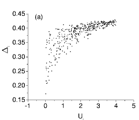
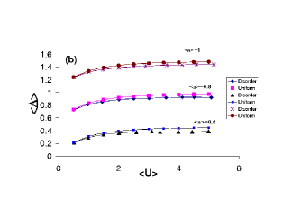
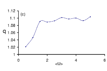
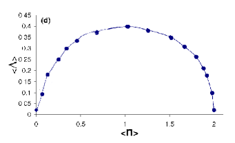
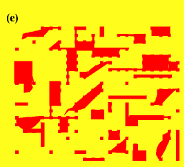
Figure 1: (Colour online) (a)Variation of the local pairing amplitude $\Delta_{i}$ with the interaction $U_{i}$, distributed uniformly in the range 0-4 (b)Comparison between the variation of $<\Delta>$ with $<U>$ for uniform and disordered cases at $<n>=1$, $<n>=0.8$ and $<n>=0.6$. (c)Variation of $<\Delta_{uniform}>/<\Delta_{disorder}>$with $<U>$. (d)Variation of average local pairing amplitude$<\Delta>$ with $<n>$)(e) Superconducting regions for U=0-2. The red islands represent superconducting regions with large amplitude (see text).

Fig. 1a shows that $\Delta_{i}$ increases with $U_{i}$ and saturates at large $U_{i}$, there is a broad distribution of $\Delta_{i}$ for lower values of $U_{i}$. Fluctuation in the pairing amplitude $\Delta_{i}$ are indeed larger in the weak-coupling region. The variation of the average $U_{i}$ and the average $<\Delta>=\frac{1}{N}\sum_{i}\Delta_{i}$ gives a good indication of their relationship and can be compared with the uniform case. The comparison in Fig.1b shows an enhancement of the average superconducting pairing amplitude $\langle\Delta\rangle$ with $\langle U\rangle$ as expected saturating at a higher value of the attraction. The value of average pairing amplitude is higher for the uniform case than the disorder case for all values of$<n>=1.0,0.8$ and $0.6$ contrary to that of bimodal distribution. Fig. 1c shows the ratio as a function of average interaction, and it rises sharply at low $U$ and always stays above one. This implies that the random disorder inhibits long range superconducting order. Fig.1d shows the usual bell-shaped curve of $<\Delta>$ versus $<n>$ with maximum at $<n>=1$.

In order to glean the real-space picture of the superconducting regions, we mark the sites where the value of $\Delta_{i}$ is greater than the corresponding value in the homogeneous case (Fig.1e). Since all sites have non-zero $\Delta_{i}$, this prescription allows us to locate preferred patterns, if any, in the real space. We do not see any such pattern while the regions of strong $\Delta_{i}$ are quite randomly distributed forming patches. The formation of islands in turn reduces the overall observed $T_{c}$ (which is determined by the phase coupling across such regions) in a real system and the corresponding superfluid stiffness.

Plotting the frequency distribution of $\Delta_{i}$ gives a good account of the effects of disorder. The peak in Fig. 2a is certainly above the mean value. With higher disorder the peak shifts towards right. Further on we calculate the pair correlation function (Fig. 2b), defined as $c(r_{i}-r_{j})=<\Delta_{i}\,\Delta_{j}>$. A disorder averaging is done as usual to restore the translational invariance. The correlation function drops sharply at short distances but saturates at large distances indicating a true (mean-field) long range order. The correlation function for four ranges of $U$ are shown in Fig. 2b, they all merge to a single curve (except for small fluctuations due to finite size) when normalized.

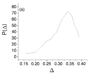
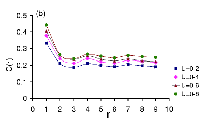
Figure 2: (a)Frequency Distribution P($\Delta$) of $\Delta$ for U=0-2 (b)Plot of correlation for four U ranges: 0-2 0-4 0-6 0-8

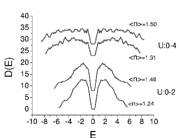
Figure 3: Density of States plot for U=0-2 and 0-4, the two sets of curves are offset vertically to make them separate.

The presence of a superconducting gap is another indication of the true long range order [9]. It is, therefore, very important to look at the density of states (DOS) of the system. As mentioned above there are no sites with zero pairing amplitude. This is reflected in the DOS where the gap at zero energy is clearly seen in Fig. 3, while the very sharp peaks (divergences in a homogeneous superconductor) are now broadened into two symmetrical regions with a broad distribution of states at higher and lower energies. The presence of the energy gap even in the highly disordered systems clearly indicates that s-wave superconductivity is possible even in the presence of large disorder.

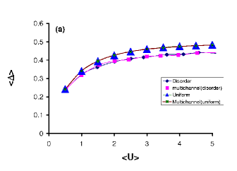
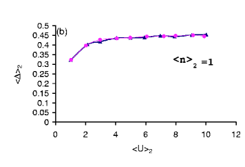
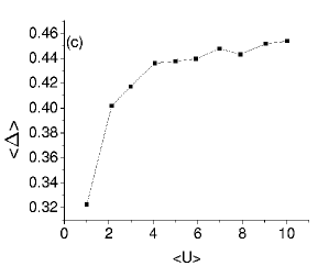
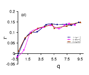
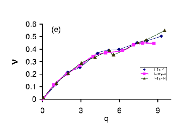
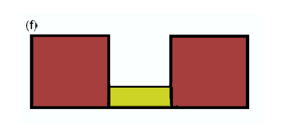
Figure 4: (a)Variation of $<\Delta>$ with $<U>$ for individual blocks of the coupled system for both disorder and uniform case and its comparison with single block system. (b) $\langle\Delta\rangle_{2}$ as a function of $\langle U\rangle_{2}$ for $\langle n\rangle_{2}=1$ and comparison with superconductivity in a single system. (c) $\langle\Delta\rangle$ as a function of $\langle U\rangle$ with $\langle n\rangle=1$ for the whole system. (d) Variation of $\Gamma=\langle\Delta\rangle_{2}-\langle\Delta\rangle_{1}$ with $q=\langle U\rangle_{2}-\langle U\rangle_{1},\,\langle n\rangle=1$. Here the legend $l$ refers to length of channel and $y$ refers to its width. (e) Variation of $\nu=\langle n\rangle_{2}-\langle n\rangle_{1}$ with $q$ while $\langle n\rangle=1.$ (f) Two superconducting blocks connected by a channel

To understand the effect of coupling of two disordered superconductors, we take up two such superconductors and join them via a narrow channel (Fig. 4f) and observe the effects due to the proximity of each other. We find that contrary to the common expectation the width and length of the channel do not have any significant effect on the superconductivity in either systems (4d,e).More interestingly, results from the comparative variation of $\langle\Delta\rangle,\langle U\rangle,\langle n\rangle$ of the two blocks (Fig. 4a-e) do not give any clear influence of the channel. For example, we observed the variation of $\langle\Delta\rangle$ of one superconductor with the $\langle U\rangle$ in both uniform and disordered case and compared with similar results of the single block system we had obtained earlier. Results are symmetric with respect to interchange of systems 1 and 2. It is clearly seen from Fig. 4a that the average superconducting pairing amplitude in blocks of the coupled system follow identically the pattern of a single block system in both disorder and uniform regime. The channel was kept homogeneous. The results do not change if the channel is maintained homogeneous but non superconducting ($U_{i}=0$ for all $i$ in the channel).This unexpected behaviour, we believe, is due to the formation of islands of low pairing amplitude discussed earlier (Fig 1e). These regions localize the electron in the block since it would be energetically unfavourable for the electrons to percolate through the channel. This inhibits correlations between the blocks,effectively making them behave as independent systems.

The average superconducting pairing amplitude in the second system increases at the expense of $\langle\Delta_{1}\rangle$ (Fig. 4b since the enhanced attraction in system 2 provides extra stabilization energy in that region. Note that the variation of $<\Delta_{2}>$ with $<U_{2}>$ is also unaffected (Fig. 4b) by the presence of system 1 and nearly similar to that for a single system. The variations of overall average pairing amplitude $\langle\Delta_{1}+\Delta_{2}\rangle$ with total average interaction at a fixed overall density is shown in Fig. 4c. The combined system behaves like an isolated single system and expectedly shows the typical rise and saturation behaviour seen in a single system.

Fig. 4d demonstrates clearly how the average order parameter in the two systems are correlated with the corresponding interactions. The larger the attraction, more is the average $\langle\Delta\rangle$. As $\langle U\rangle$ increases in any system, the density of electrons tends to increase for the extra stabilization available in that region. Fig. 4e shows this tendency, with $\langle n_{i}\rangle$ in each superconductor increasing rapidly with the average attractive interaction there.

4 Conclusion

In conclusion, we have studied inhomogeneous s-wave superconductors using the Bogoliubov de-Gennes mean-field theory. Superconductivity is suppressed over the homogeneous weak-coupling value due to disorder, though the proximity effect is strong with non-zero pairing amplitude at all sites (even with $U_{i}=0$). The frequency distribution of $p(\Delta)$ shows a peak towards higher values of $\Delta$. The gap in the density of states persists even for the high disordered case lending support to the existence of strongly disordered inhomogeneous superconductivity. When two such blocks of inhomogeneous superconductors are connected via a channel, there is no appreciable effect of one on the other. The individual blocks are not affected significantly by the other block connected by the channel . We argue that this is due to the fact that the fluctuating local order parameters remain pinned to the individual values thereby preventing significant correlation between the blocks.

5 Acknowledgment

BC acknowledges a junior research fellowship from the Council of Scientific and Industrial Research, India.

References

- [1] D. Belitz and T. R. Kirkpatrick, Rev. Mod. Phys. 66, 261 (1994).
- [2] K. McElroy, D.-H. Lee, J. E. Hoffman, K. M. Lang, J. Lee, E. W Hudson, H. Eisaki, S. Uchida, and J. C. Davis, Phys. Rev. Lett 94, 197005 (2005) .
- [3] H. A. Mook, P. Dai, and F. Dogan, Phys. Rev. Lett. 88, 09700 (2002) .
- [4] T. Hanaguri, C. Lupien, Y. Kohsaka, D.-H. Lee, M. Azuma, M Takano, H. Takagi, and J. C. Davis, Nature London 430, 100 (2004).
- [5] J. M. Tranquada, J. D. Axe, N. Ichikawa, A. R. Moodenbaugh, Y Nakamura, and S. Uchida, Phys. Rev. Lett. 78, 338 (1997) .
- [6] Ch. Renner, G. Aeppli, B.-G. Kim, Y.-A. Soh, and S.-W. Cheong Nature London 416, 518 (2002) .
- [7] A. J. Millis, Science, 314, 1888 (2006).
- [8] K. Aryanpour, E. R. Dagotto, M. Mayr, T. Paiva, W. E. Pickett, R. T. Scalettar, Phys. Rev. B 73, 104518 (2006).
- [9] A. Ghosal, M. Randeria and N. Trivedi, Phys. Rev. B 65, 014501 (2002).
- [10] K. Machida, Physica C 158, 192 (1989).
- [11] M. Kato, K. Machida, H. Nakanishi, and M. Fujita, J. Phys. Soc. Jpn. 59, 1047 (1990) .
- [12] S. R. White and D. J. Scalapino, Phys. Rev. B 70, 220506 (2004).
- [13] M. Voita, Phys. Rev. B 66, 104505 (2002).
- [14] I. Martin, D. Podolsky and S. A. Kivelson, Phys. Rev. B 72, 060502 (2005).
- [15] V. J. Emery and S. A. Kivelson, Nature 374, 434 (1995); V. J. Emery and S. A. Kivelson and O. Zachar, Phys. Rev. B 56, 6120 (1997).
- [16] A. Taraphder, H.R. Krishnamurthy, R. Pandit, and T. V. Ramakrishnan, Phys. Rev. B, 52 1368-1388 (1995).
- [17] A. Taraphder, H.R. Krishnamurthy, R. Pandit, and T. V. Ramakrishnan, Int. J. Mod. Phys., 10, 863-954 (1996).