Field sweep rate dependence of magnetic domain patterns: Numerical simulations for a simple Ising-like model

Abstract

We study magnetic domain patterns in ferromagnetic thin films by numerical simulations for a simple Ising-like model. Magnetic domain patterns after quench demonstrate various types of patterns depending on the field sweep rate and parameters of the model. How the domain patterns are formed is shown with the use of the number of domains, the domain area, and domain-area distributions, as well as snapshots of domain patterns. Considering the proper time scale of the system, we propose a criterion for the structure of domain patterns.

I Introduction

Various kinds of domain pattern are seen in a large number of physical and chemical systems and have been investigated experimentally, numerically, and theoretically.cross ; seul Magnetic domain patterns in uniaxial ferromagnetic garnet thin films also show many types of structure. For example, a hexagonal or square lattice, bubbles, stripes, and so on are observed under static or oscillating magnetic field perpendicular to the film plane. Under zero field, after quench, a labyrinth structure is often observed. In some cases, the domain pattern under zero field has a sea-island structure, which consists of many small up-spin (down-spin) “islands” (domains) surrounded by the “sea” of down (up) spins. Labyrinth and sea-island structures are metastable patterns and should change to a parallel-stripe structure under the thermal fluctuation or other kinds of fluctuation. In fact, it was observed in experiments that a labyrinth structure changes to a parallel-stripe structure under field cycles.miura ; mino

Magnetic domain patterns show different structures depending on the external field. There are several simulations which demonstrate how domain patterns change under very slowly changing field.jagla04 ; jagla05 ; deutsch Some of them also showed hysteresis curves.jagla05 ; deutsch Though a hysteresis curve has no information about the structure of a domain pattern, it gives information about magnetic ordering. Magnetic ordering depends not only on the external field but also on the field changing rate. In fact, there are also some works about the dependence of hysteresis on the frequency and amplitude of an oscillating field.luse ; sides ; jang

In this paper, we focus on the domain patterns under zero field and study them by numerical simulations. Our model is a simple Ising-like model which reproduces domain patterns observed in experiments for ferromagnetic garnet thin films. In experiments, domain patterns under zero field are observed after a strong applied field is switched off. Therefore, we need to start a simulation from the state under magnetic field above the saturation field in order to reproduce the domain pattern under zero field. Recently, the field sweep-rate dependence of domain patterns was studied experimentally and numerically in Ref. kudo, . However, the parameters except for the field sweep rate were fixed to specific values in the simulations. The parameters are different among samples in experiments. Here, we will also study a parameter dependence of domain patterns. The parameter dependence as well as the field sweep-rate dependence may give useful information on rich properties of the pattern formation in a ferromagnetic thin film.

The rest of this paper is organized as follows. In Sec. II, we describe our model and numerical procedure. In Secs. III and IV, the characteristics of domain patterns are displayed for fast- and slow-quench cases, respectively. We will show not only snapshots of domain patterns but also the number of domains, domain areas, and the domain-area distributions. Such quantities enable us to picture how the domain patterns appear. In Sec. V, a criterion about domain patterns and the field sweep rate is discussed. Conclusions are given in Sec. VI.

II Model and numerical procedure

Our model is a simple two-dimensional Ising-like model whose Hamiltonian consists of four energy terms: uniaxial-anisotropy energy $H_{\rm ani}$, local ferromagnetic interactions (exchange interactions) $H_{J}$, long range dipolar interactions $H_{\rm di}$, and interactions with the external field $H_{\rm ex}$.jagla04 ; jagla05 ; kudo ; elias ; sagui We consider a scalar field $\phi(\bm{r})$, where $\bm{r}=(x,y)$. The positive and negative values of $\phi(\bm{r})$ correspond to up and down spins, respectively. The anisotropy energy prefers the values $\phi(\bm{r})=\pm 1$:

$$H_{\rm ani}=\alpha\int{\rm d}\bm{r}\left(-\frac{\phi(\bm{r})^{2}}{2}+\frac{\phi(\bm{r})^{4}}{4}\right).$$ (1)

The exchange and dipolar interactions are described by

$$H_{J}=\beta\int{\rm d}\bm{r}\frac{|\nabla\phi(\bm{r})|^{2}}{2}$$ (2)

and

$$H_{\rm di}=\gamma\int{\rm d}\bm{r}{\rm d}\bm{r}^{\prime}\phi(\bm{r})\phi(\bm{r}^{\prime})G(\bm{r},\bm{r}^{\prime}),$$ (3)

respectively. Here, $G(\bm{r},\bm{r}^{\prime})\sim|\bm{r}-\bm{r}^{\prime}|^{-3}$ at long distances. The exchange and dipolar interactions may be interpreted as short-range attractive and long-range repulsive interactions. Namely, $\phi(\bm{r})$ tends to have the same value as neighbors because of the exchange interactions, and it also tends to have the opposite sign to the values in a region at a long distance because of the dipolar interactions. These two interactions play an important role in creating a domain pattern with a characteristic length. The term from the interactions with the external field is given by

$$H_{\rm ex}=-h(t)\int{\rm d}\bm{r}\phi(\bm{r}),$$ (4)

where $h(t)$ is the time-dependent external field. Here, let us introduce a disorder effect. In other words, spatial randomness is introduced in the model. We consider the disorder effect only in the anisotropy term: $\alpha$ is replaced by $\alpha\lambda(\bm{r})$, where

$$\lambda(\bm{r})=1+\mu(\bm{r})/4.$$ (5)

Here, $\mu(\bm{r})$ is an uncorrelated random number with a Gaussian distribution whose average and variance are 0 and $\mu_{0}^{2}$, respectively. However, $\mu(\bm{r})$ should have a cutoff so that $\lambda(\bm{r})$ is always positive. In our simulations, we set $\mu_{0}=0.3$. From Eqs. (1)–(5), the dynamical equation of our model is described by

$$\frac{\partial\phi(\bm{r})}{\partial t} = -L_{0}\frac{\delta(H_{\rm ani}+H_{J}+H_{\rm di}+{H_{\rm ex}})}{\delta\phi(\bm{r})}$$ (6)

$$= L_{0}\biggl{\{}\alpha\lambda(\bm{r})[\phi(\bm{r})-\phi(\bm{r})^{3}]+\beta\nabla^{2}\phi(\bm{r})-\gamma\int{\rm d}\bm{r}^{\prime}\phi(\bm{r}^{\prime})G(\bm{r},\bm{r}^{\prime})+h(t)\bigg{\}}.$$

Hereafter, we fix $L_{0}=1$.

It is useful to calculate the time evolutions of Eq. (6) in Fourier space when we perform numerical simulations. The equation is rewritten as

$$\frac{\partial\phi_{\bm{k}}}{\partial t}=\alpha[(\phi-\phi^{3})\lambda]_{\bm{k}}-(\beta k^{2}+\gamma G_{\bm{k}})\phi_{\bm{k}}+h(t)\delta_{\bm{k},0},$$ (7)

where $[\cdot]_{\bm{k}}$ denotes the convolution sum and $G_{\bm{k}}$ is the Fourier transform of $G(\bm{r},0)$. If $G(\bm{r},0)\equiv 1/|\bm{r}|^{3}$, then

$$G_{\bm{k}}=a_{0}-a_{1}k,$$ (8)

where $k=|\bm{k}|$ and

$$a_{0}=2\pi\int_{d}^{\infty}r{\rm d}rG(r),\quad a_{1}=2\pi.$$ (9)

Here, $d$ is the cutoff length, which can be interpreted as the lower limit of the dipolar interactions. In fact, $G(\bm{r},0)$ cannot be assumed to be $1/|\bm{r}|^{3}$ at short distances, and Eq. (8) is the asymptotic form for $k\to 0$. However, the details of $G(\bm{r},0)$ is not important at short distances because the exchange interactions (the $k^{2}$ term) are dominant there. In the simulations below, we use Eqs. (8) and (9) as $G_{\bm{k}}$ and set $d=\pi/2$, which results in $a_{0}=4$.

Equation (7) is useful also for discussing some characteristic properties of domain patterns. Let us consider only linear terms in the equation

$$\frac{\partial\phi_{\bm{k}}}{\partial t}=\eta_{\bm{k}}\phi_{\bm{k}},$$ (10)

where $\eta_{\bm{k}}$ is the linear-growth rate for zero field. It means that $\phi_{\bm{k}}$ decays exponentially for negative $\eta_{\bm{k}}$ and grows exponentially for positive $\eta_{\bm{k}}$, although the nonlinear term prevents $\phi_{\bm{k}}$’s growing too much. The linear-growth rate has a quadratic maximum:

$$\eta_{\bm{k}} = -(\beta k^{2}-\gamma a_{1}k+\gamma a_{0})+\alpha$$ (11)

$$= -\beta\left(k-\frac{a_{1}\gamma}{2\beta}\right)^{2}+\frac{a_{1}^{2}\gamma^{2}}{4\beta}-\gamma a_{0}+\alpha.$$

This suggests that the characteristic length of the domain patterns should be $2\pi/k_{0}$, where $k_{0}=a_{1}\gamma/2\beta$. Therefore, if the values of $\beta$ and $\gamma$ are fixed, the characteristic length should be also fixed. In our simulations, we give those values as $\beta=2.0$ and $\gamma=2\beta/a_{1}=2.0/\pi$, so that $k_{0}=1.0$. On the other hand, one of the central subjects in this paper is the $\alpha$ dependence of domain patterns. When $\alpha$ becomes large, the $k$ region with positive $\eta_{\bm{k}}$ broadens and many modes of $\eta_{\bm{k}}$ grow. Therefore, the surface of domains can be rough for large $\alpha$.

In this paper, we consider a descending field as the external field

$$h(t)=h_{\rm ini}-vt,$$ (12)

where $h_{\rm ini}$ is the initial external field, which should be equal to or larger than the saturating field. The value of the saturating field can be estimated from a simulation under ascending field as follows. After a domain pattern is formed spontaneously under zero field, an increasing field is applied. At a certain value of $h$, the domains with negative $\phi(\bm{r})$ disappear. Then, we consider this value as the saturating field. Although the saturating field depends on $\alpha$, we set $h_{\rm ini}=1.5$ for all values of $\alpha$ in our simulations, so that $h_{\rm ini}$ is larger than the saturation fields for all $\alpha$.

The details of the numerical procedure is as follows. As the initial condition, $\phi(\bm{r})$ is given by random numbers in the interval $1.0<\phi(\bm{r})<1.1$ at $t=0$. The external field decreases from $h_{\rm ini}$ to $0$, following Eq. (12). Once the external field becomes zero at $t_{0}=h_{\rm ini}/v$, the field remains zero for $t_{0}\leq t\leq 2t_{0}$. Namely, we stop the calculation at $2t_{0}$. The time evolution is calculated by using a semi-implicit method. In other words, while we use the exact solutions for the linear and field terms, the second order Runge-Kutta method is applied to the calculation for the nonlinear term. The semi-implicit method enables us to use a rather large time interval: $\delta t=0.1$ in the simulations below. The simulations are performed on a $512\times 512$ lattice with periodic boundary conditions.

III Fast quench

In this section, we focus on the fast-quench case where the sweep rate of the field is $v=10^{-2}$. The scale of the field sweep rate will be elucidated in Sec. V. Considering the results in Ref. kudo, , we expect that some kinds of sea-island structure should appear in this case. It will be shown how the characteristics of domain patterns depend on the anisotropy parameter $\alpha$. The characteristics are demonstrated by the snapshots of domain patterns, the total number of domains, average domain area, and domain-area distributions.

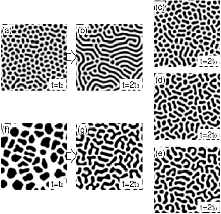
Figure 1: Domain patterns under zero field after a fast quench ($v=10^{-2}$), which display the dependence on the parameter $\alpha$: [(a) and (b)] $\alpha=1.5$, (c) $\alpha=2.0$, (d) $\alpha=2.5$, (e) $\alpha=3.0$, and [(f) and (g)] $\alpha=3.5$. They are the patterns at $t=2t_{0}$ except for (a) and (f); these two are the ones at $t=t_{0}$. The size of the snapshots is $96\times 96$, although the system size is $512\times 512$. The value of $\phi(\bm{r})$ is positive and negative in the white and black areas, respectively.

Figure 1 shows the domain patterns under zero field. The white and black areas correspond to positive and negative $\phi(\bm{r})$, i.e., up and down spins, respectively. For $\alpha=1.5$ and $\alpha=3.5$, the domain patterns considerably change after the external field becomes zero at $t=t_{0}$. By contrast, little additional change in domain patterns can be seen for $\alpha=2.0$, $2.5$, and $3.0$, so that the snapshots for them are displayed only for $t=2t_{0}$. When $\alpha=1.5$, black domains connect with each other due to the exchange interactions [see Figs. 1(a) and 1(b)]. In the other cases (i.e., for $\alpha=2.0$, $2.5$, $3.0$, and $3.5$), the domains do not tend to connect because of the dipolar interactions. However, the exchange interactions prefer connection of domains, and it is preferable in the viewpoint of energy. When $\alpha$ is small, the exchange interactions are relatively large and domains can connect with each other, though the coalescence of domains causes temporary energy loss of the dipolar interactions. For $\alpha=3.5$, after large black domains appear [Fig. 1(f)], their shape changes to be like an island with the same characteristic width as in other cases [compare Fig. 1(g) with Figs. 1(c)–1(e)].

From Fig. 1, one should notice the following: the larger $\alpha$, the more inhomogeneous width of black domains. Namely, some domains are partly narrow or thick when $\alpha$ is large. The property can be explained by the linear-growth rate, Eq. (11). When $\alpha$ becomes large, the maximum value of $\eta_{\bm{k}}$ also becomes large. Then, the $k$ region where $\eta_{\bm{k}}>0$ broadens. Therefore, $\phi_{\bm{k}}$’s with different values of $\bm{k}$ grow and make the domain patterns with inhomogeneous thickness. The large black domains in Fig. 1(f) are also explained in the same way. After some time, Fig. 1(f) changes into Fig. 1(g) because a structure composed of domains whose characteristic length is $2\pi/k_{0}$ is more stable than the one composed of large round domains.

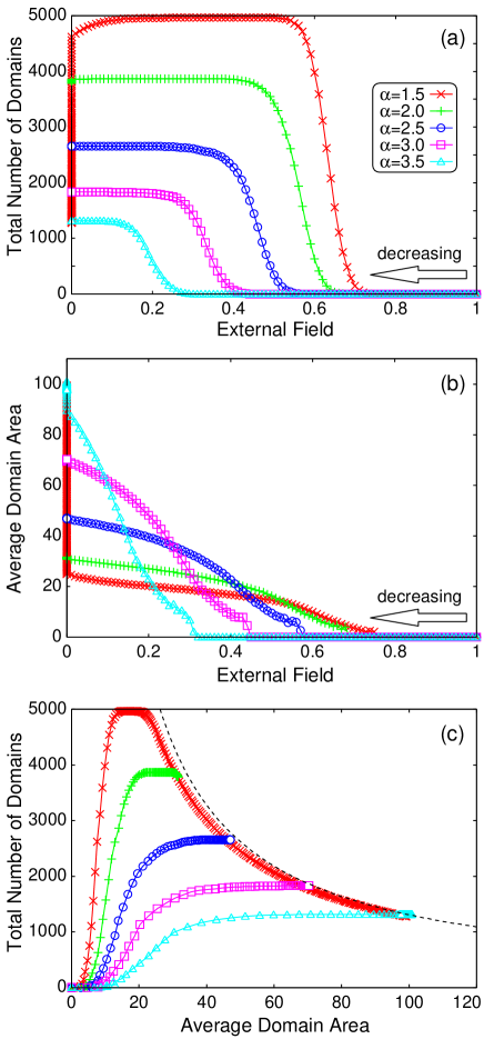
Figure 2: (Online color) The field dependence of (a) the total number of domains $N_{\rm tot}$ and (b) the average domain area $A_{\rm av}$; (c) the $A_{\rm av}$-$N_{\rm tot}$ graph. The broken line in (c) expresses the curve of $A_{\rm av}N_{\rm tot}=512^{2}/2$, where the total areas of black and white domains are equal. The calculation was performed under a rapidly decreasing field ($v=10^{-2}$) until $t=t_{0}$ and then under zero field until $t=2t_{0}$. The number of domains means the number of negative-$\phi(\bm{r})$ (black) domains. The domain area is the number of grid points that have negative values of $\phi(\bm{r})$.

The field dependence of the total number $N_{\rm tot}$ and average area $A_{\rm av}$ of negative-$\phi(\bm{r})$ (black) domains is shown in Figs. 2(a) and 2(b). Under a decreasing field, $N_{\rm tot}$ starts increasing at a certain field and stops increasing at another low field. In the plateau region of $N_{\rm tot}$, each domain grows and $A_{\rm av}$ keeps increasing. When $\alpha=1.5$, $N_{\rm tot}$ starts to decrease after the plateau region. Moreover, for $\alpha=1.5$, $N_{\rm tot}$ and $A_{\rm av}$ keep decreasing and increasing, respectively, after the external field becomes zero. This behavior is caused by connection of domains as mentioned above: cf. Figs. 1(a) and 1(b). If the calculation is continued for $t\geq 2t_{0}$, the values of $N_{\rm tot}$ and $A_{\rm av}$ will decrease and increase more, respectively. On the other hand, when $\alpha=3.5$, $A_{\rm av}$ increases also after the external field reaches zero, although $N_{\rm tot}$ does not change under zero field. This means that each domain just grows without increase of the number of domains. For $t\geq 2t_{0}$, $A_{\rm av}$ does not increase when $\alpha=3.5$. In fact, $A_{\rm av}$ of $\alpha=3.5$ has the maximum value at a certain time between $t_{0}$ and $2t_{0}$.

Figure 2(a) also enables us to know that the larger the $\alpha$, the lower the value of the external field where the first black domain appears. This fact implies that spins cannot easily flop when $\alpha$ is large. In other words, for large $\alpha$, the minima of $H_{\rm ani}$ are low and the transition between negative- and positive-$\phi(\bm{r})$ states does not easily occur. Another point we notice about Fig. 2(a) is that the larger the $\alpha$, the smaller the $N_{\rm tot}$. This can be explained by the linear growth rate, Eq. (11). As mentioned above, the $k$ region where $\phi_{\bm{k}}>0$ broadens when $\alpha$ becomes large. Therefore, the size of each domain can become large for large $\alpha$. If the size of each domain is large, the number of domains should be small.

Figure 2(c) shows the $A_{\rm av}$-$N_{\rm tot}$ graph. The broken line is the curve of $A_{\rm av}N_{\rm tot}=512^{2}/2$, where the total numbers of the black and white domains are equal. The curve for each $\alpha$ starts at $(A_{\rm av},N_{\rm tot})=(0,0)$ and approaches the broken line. The curve for $\alpha=2.0$ and $\alpha=2.5$ do not reach the broken line, which means that there is a remanent magnetization.

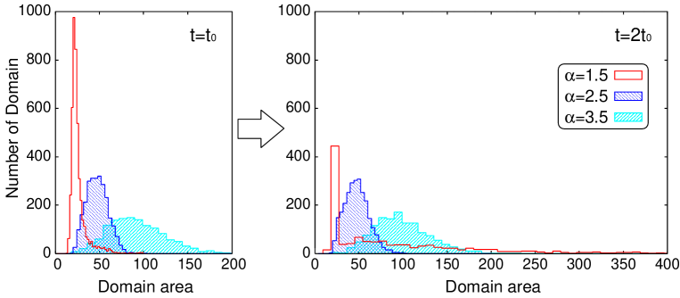
Figure 3: (Online color) Domain-area distributions at $t=t_{0}$ and $t=2t_{0}$. The left, center, and right histograms at each time are for $\alpha=1.5$, $\alpha=2.5$, and $\alpha=3.5$, respectively. The domain area is the number of grid points that have negative values of $\phi(\bm{r})$.

Figure 3 displays the domain-area distributions at $t=t_{0}$ and $2t_{0}$ for $\alpha=1.5$, $2.5$, and $3.5$. The distribution for $\alpha=1.5$ at $t=t_{0}$ has a sharp peak at a certain small value of domain area. The peak falls and a long tail appears at $t=2t_{0}$. This change reflects the connection of domains for $\alpha=1.5$ as mentioned above. For $\alpha=2.5$ or $\alpha=3.5$, the shape of the each distribution is similar to a Gaussian distribution and its change between $t=t_{0}$ and $t=2t_{0}$ is small. Here, we note that the larger the $\alpha$, the broader the distribution appears. It can also be explained by the linear-growth rate.

IV Slow quench

In this section, we show our results for the slow-quench case where the field sweep rate is $v=10^{-4}$. Considering the results in Ref. kudo, , we expect some kinds of labyrinth structure in this case. The dependence on $\alpha$ of the characteristics of domain patterns is demonstrated by the snapshots of domain patterns, the total number of domains, and average domain area. Here, domain-area distributions are not displayed since each domain can grow too long under the slowly descending field.

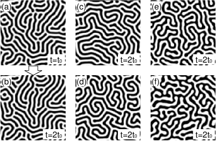
Figure 4: Domain patterns under zero field after a slow quench ($v=10^{-4}$), which display the dependence on the parameter $\alpha$: [(a) and (b)] $\alpha=1.5$, (c) $\alpha=2.0$, (d) $\alpha=2.5$, (e) $\alpha=3.0$, and (f) $\alpha=3.5$. They are the patterns at $t=2t_{0}$ except for (a) at $t=t_{0}$.

Figure 4 shows the domain patterns under zero field. In contrast to the fast-quench case, the domain patterns for $\alpha=1.5$ do not change so much between $t=t_{0}$ and $t=2t_{0}$. It is because the connection of domains has almost finished by $t=t_{0}$. In fact, the connection of many small domains happens also in this case for $\alpha=1.5$ (see Fig. 5). On the other hand, when $\alpha$ is large, the width of black domains is inhomogeneous. This property is the same as the fast-quench case. We should note another property: There are many branches of black domains for large $\alpha$. It is related to the inhomogeneity of domain width. As black domains grow, they bifurcate at the place where the domain width becomes large.

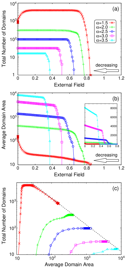
Figure 5: (Online color) The field dependence of (a) the total number of domains $N_{\rm tot}$ and (b) the average domain area $A_{\rm av}$; (c) the $A_{\rm av}$-$N_{\rm tot}$ graph. The calculation was performed under a slowly decreasing field ($v=10^{-4}$) until $t=t_{0}$ and then under zero field until $t=2t_{0}$. The data are displayed on a semilogarithmic scale in (a) and (b) and on a log-log scale in (c), while the inset of (b) shows the same data as its main panel on a normal scale. The broken line in (c) expresses the curve of $A_{\rm av}N_{\rm tot}=512^{2}/2$.

The field dependence of the total number $N_{\rm tot}$ and average area $A_{\rm av}$ of black domains is shown on a semilogarithmic scale in Figs. 5(a) and 5(b). Also, in this slow-quench case, $N_{\rm tot}$ decreases after the plateau region for $\alpha=1.5$ because of the connection of domains. Though $N_{\rm tot}$ decreases and $A_{\rm av}$ increases after the external field becomes zero for $\alpha=1.5$, they change very little for $t\geq 2t_{0}$. Comparing Fig. 5 with Fig. 2, we find two things. First, the difference between both data for $\alpha=1.5$ is rather small. Second, the larger the $\alpha$, the larger the difference. The dependence on the field sweep rate was discussed in Ref. kudo, only in the specific case of $\alpha=2.5$. Although the discussion is basically applicable for other values of $\alpha$, little difference appears for small $\alpha$ because spins can flop easily regardless of the field sweep rate.

The inset of Fig. 5(b) shows the field dependence of $A_{\rm av}$ on normal scale. For $\alpha$ larger than $2.0$, $A_{\rm av}$ grows linearly in the low field region. The linear-growth region of $A_{\rm av}$ is within the plateau region of $N_{\rm tot}$. This means that the magnetization linearly decreases in that region as the external field decreases.

Figure 5(c) shows the $A_{\rm av}$-$N_{\rm tot}$ graph on a log-log scale. The end of each curve is almost on the broken line which expresses the zero magnetization. In other words, the remanent magnetization is almost zero in this case.

V Criterion for the domain structure and standard parameter for the field sweep rate

Now, let us consider the dependence on the field sweep rate. Some discussion about it was given in Ref. kudo, . Namely, sea-island and labyrinth structures appear under zero field for rapidly and slowly decreasing fields, respectively. Such behavior was explained by the concept of crystallization: For a fast-quench case, high “supersaturation” lowers the nucleation energy, while the nucleation energy is high for a slow-quench case.kudo When the nucleation energy is small, many domains appear at once and cannot grow so long. By contrast, when the nucleation energy is large, a small number of domains appear and can grow very long. However, these discussions were just qualitative ones, and no standard parameter responsible to the field sweep rate has been provided.

In order to predict the domain pattern in experiments, a criterion about the dependence on the field sweep rate should be elucidated. Since the proper time scale of each sample is different, the balance between the proper time scale and the field sweep rate must be considered to give the criterion. The proper time scale is related to $L_{0}$ of Eq. (6), while we set $L_{0}=1$ in the simulations. First, we should scale out $L_{0}$ and a parameter $\beta$ in Eq. (6). If we write $\tilde{t}\equiv L_{0}\beta t$, then Eq. (6) becomes

$$\frac{\partial\phi(\bm{r})}{\partial\tilde{t}}=\tilde{\alpha}\lambda(\bm{r})[\phi(\bm{r})-\phi(\bm{r})^{3}]+\nabla^{2}\phi(\bm{r})-\tilde{\gamma}\int{\rm d}\bm{r}^{\prime}\phi(\bm{r}^{\prime})G(\bm{r},\bm{r}^{\prime})+\tilde{h}(\tilde{t}),$$ (13)

where $\tilde{\alpha}=\alpha/\beta$, $\tilde{\gamma}=\gamma/\beta$, and

$$\tilde{h}(\tilde{t})=\frac{h_{\rm ini}}{\beta}-\frac{v}{L_{0}\beta^{2}}\tilde{t}.$$ (14)

Here, let us call $\tilde{v}\equiv v/(L_{0}\beta^{2})$ a scaled sweep rate of the external field. Next, we have to decide the crossover sweep rate $v_{c}$ as well as the scaled one $\tilde{v}_{c}$. Here, crossover means the crossover from a sea-island structure to a labyrinth structure. Then, the value of $v/v_{c}$ becomes a rough standard in distinguishing sea-island and labyrinth structures. If $L_{0}$ and $\beta$ of a sample could be measured in experiments, $v_{c}$ of the sample would be obtained from $\tilde{v}=v/(L_{0}\beta^{2})$. Then, we can predict the pattern for an actual $v$ from the value of $v/v_{c}$.

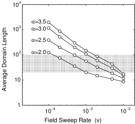
Figure 6: Dependence of the average domain length at $t=2t_{0}$ on the field sweep rate $v$. The average domain length is calculated from the average domain area and the average domain width (see text). The domain pattern looks like labyrinth and sea-island structures above and below the gray patched area, respectively.

We need to consider how to distinguish sea-island and labyrinth structures. Let us introduce the average domain length as a quantity to distinguish them, which can be obtained by dividing the average domain area by the average domain width. For each $\alpha$ and $v$, the average domain width was calculated from the autocorrelation function at $t=2t_{0}$. In Fig. 6, the average domain length is plotted against the field sweep rate for $\alpha=2.0$, 2.5, 3.0, and 3.5. Recalling the snapshots in Figs. 1 and 4, we can expect labyrinth and sea-island structures above and below the gray patched area, respectively. Here, we define $v_{c}=10^{-3}$ in this case, although it is not a clear crossover point. Then, the crossover sweep rate in another case is estimated by $v_{c}=\tilde{v}_{c}L_{0}\beta^{2}=2.5\times 10^{-4}\times L_{0}\beta^{2}$.

Now, let us introduce a parameter $\kappa=\log_{10}(v/v_{c})$. Then, we can expect that a sea-island structure appears for about $\kappa\geq 1$ and labyrinth one for about $\kappa\leq-1$. In fact, the experimental results of Ref. kudo, support the expectation: Sea-island structure appeared for $2\times 10^{5}$ Oe/s and labyrinth structure for $10$ Oe/s. Although we do not know the value of $v_{c}$ in that case, it is certain that the difference between the values of $\kappa$ for sea-island and labyrinth structures is more than 2 [$=1-(-1)$]. Therefore, we suggest that the parameter $\kappa$ should be a useful standard parameter to distinguish sea-island and labyrinth structures.

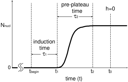
Figure 7: Schematic picture about the characteristic times in the nucleation process. See text for the details.

Here, we explain a linear decay on the logarithmic scale in the field sweep-rate dependence of the average domain length ($\ell_{\rm av}$) in Fig. 6. Let us recall that the data in Fig. 6 are confined to the cases where the total number of domains does not change after the external field vanishes [see Figs. 2(a) and 5(a)]. $\ell_{\rm av}$ is inversely proportional to the number of domains ($N_{\rm tot}$), which is equal to that of the created nuclei ($N_{\rm nucl}$) since no connection of domains occurs in the cases investigated in Fig. 6. As $N_{\rm nucl}$ is proportional to the degree of supersaturation ($\Delta F$), the evaluation of $\ell_{\rm av}$ is eventually reduced to that of $\Delta F$. Now, we consider two characteristic times needed to explain Fig. 6: the induction time ($\tau_{1}$) and the preplateau time ($\tau_{2}$). Figure 7 illustrates the important stages of nucleation, including those times. The induction time starts at $t_{\rm begin}$, when the supersaturation begins, and ends at $t_{1}$, when the first nucleus appears, i.e., $\tau_{1}=t_{1}-t_{\rm begin}$. The preplateau time starts at $t_{1}$ and ends at $t_{2}$, when $N_{\rm nucl}(=N_{\rm tot})$ begins to take the plateau value shown in Figs. 2(a), 5(a), and 7, i.e., $\tau_{2}=t_{2}-t_{1}$. Then, $\Delta F$ is divided in two parts, $\Delta F_{1}$ and $\Delta F_{2}$: $\Delta F_{1}$ and $\Delta F_{2}$ are the partial degrees of supersaturation during the induction time ($\tau_{1}$) and the preplateau time ($\tau_{2}$), respectively.

We now proceed in estimating $\Delta F_{1}$ by comparing the energies of states (A) and (B) without and with a nucleus, respectively: (A) all spins are up, i.e., $\phi(\bm{r})=+1$ everywhere; (B) there is a circular nucleus with radius $R_{0}$ where spins are down among up spins. Namely, $\phi(\bm{r})=-1$ and $+1$ inside and outside of the nucleus in (B). In both (A) and (B), the anisotropy energy is the same: $H_{\rm ani}=-\alpha S/4$, where $S$ is the area of the system. In (A), $H_{J}=0$, $H_{\rm di}=(2\pi/d)\gamma S$, and $H_{\rm ex}=-hS$. Therefore, the energy for (A) is

$$H_{A}=-\alpha S/4+(2\pi/d)\gamma S-hS.$$ (15)

On the other hand, in (B), the dipolar interactions $H_{\rm di}$ can be estimated from the ratio of combinations of spin pairs. Since the ratio of combinations is given by the ratio of areas,

$$H_{\rm di} = (2\pi/d)\gamma S\left[\left(\frac{S-\pi R_{0}^{2}}{S}\right)^{2}+\left(\frac{\pi R_{0}^{2}}{S}\right)^{2}-2\frac{S-\pi R_{0}^{2}}{S}\frac{\pi R_{0}^{2}}{S}\right]$$ (16)

$$= (2\pi/d)\gamma S-(2\pi/d)\gamma\cdot 4\pi R_{0}^{2}\left(1-\frac{\pi R_{0}^{2}}{S}\right).$$

Then we have

$$H_{B}(t)=-\alpha S/4+(2\pi/d)\gamma S-(2\pi/d)\gamma\cdot 4\pi R_{0}^{2}\left(1-\frac{\pi R_{0}^{2}}{S}\right)-h(t)(S-2\pi R_{0}^{2}).$$ (17)

Rigorously speaking, there is an additional surface energy in (B) due to the exchange interaction ($H_{J}\sim 2\pi\beta R_{0}$), which is negligible in the present situation with $R_{0}\ll S$. When the difference between a pair of energies $H_{A}$ and $H_{B}$,

$$\Delta H_{1}(t)=H_{A}-H_{B}(t)=(2\pi/d)\gamma\cdot 4\pi R_{0}^{2}\left(1-\frac{\pi R_{0}^{2}}{S}\right)-2\pi R_{0}^{2}(h_{\rm ini}-vt),$$ (18)

is positive, it quantifies the degree of supersaturation. Noting the numerical evidence that the induction time depends on $L_{0}$ and $\alpha$ but not on $v$, we consider $\tau_{1}$ to be independent of $v$. Then, $\Delta F_{1}$ becomes

$$\Delta F_{1}=\Delta H_{1}(t_{1})=2\pi R_{0}^{2}\tau_{1}v,$$ (19)

where we used the equality $\Delta H_{1}(t_{\rm begin})=0$, i.e., there is no supersaturation at the beginning.

On the other hand, the degree of supersaturation accumulating between $t_{1}$ and $t_{2}$ is generally written by

$$\Delta F_{2}=\int^{t_{2}}_{t_{1}}{\rm d}t\left|\frac{{\rm d}}{{\rm d}t}\Delta H_{2}(t)\right|,$$ (20)

where $\Delta H_{2}(t)$ stands for the energy difference between the present state and its ideal saturated one, which correspond to multinuclei versions of $H_{A}$ and $H_{B}$ in $\Delta H_{1}$, at arbitrary time during the preplateau time. We may consider $\Delta H_{2}(t)$ as a monotonically decreasing function since the increase of nuclei reduces the degree of supersaturation and supersaturation should vanish at $t=t_{2}$. Noting $\Delta H_{2}(t_{1})=\Delta F_{1}$ and $\Delta H_{2}(t_{2})=0$, we have

$$\Delta F_{2}=\int^{t_{2}}_{t_{1}}{\rm d}t\left(-\frac{{\rm d}}{{\rm d}t}\Delta H_{2}(t)\right)=[\Delta H_{2}(t_{1})-\Delta H_{2}(t_{2})]=\Delta F_{1}.$$ (21)

From Eqs. (19) and (21), $\Delta F=2\Delta F_{1}$. Recalling the above mentioned relation ($\ell_{\rm av}\propto N_{\rm nucl}^{-1}\propto\Delta F^{-1}$), we have

$$\log_{10}\ell_{\rm av}\simeq C-\log_{10}v,$$ (22)

where $C$ is a constant. Equation (22) shows the linear decay on the logarithmic scale in Fig. 6. While this scenario has still room for improvement, it provides an essential explanation of the crossover between sea-island and labyrinth structures. The improved scenario will appear somewhere in the future.

Recently, a similar behavior to Fig. 6 was reported in quenched ferromagnetic Bose-Einstein condensations (BECs):saito The number of spin vortices in the quenched BEC depends on the quench time. The following fact was demonstrated in Ref. saito, : For a slow quench, the spin state has nearly a single-domain structure and no spin vortices appear, and some spin vortices appear for a fast quench. In other words, the faster the quench, the smaller the domain structure. The behavior is really consistent with our results. It will be an interesting problem to investigate the common mechanism of the dependence on the quench time.

VI Conclusions

We have discussed the magnetic domain patterns for several values of $\alpha$ in the cases of both fast quench and slow one. Except for $\alpha=1.5$, sea-island and labyrinth structures appear for fast- and slow-quench cases, respectively. When $\alpha=1.5$, domains connect with each other and form a labyrinth (stripelike) structure. On the other hand, when $\alpha$ is large, domains tend to have many branches and their width is inhomogeneous. We have also shown how the characteristics of the domain patterns, i.e., the number of domains and the average domain area, change under decreasing field. Moreover, we have introduced the average domain length as one of the quantities which characterize domain patterns. The dependence of the average domain length shows that the change from a labyrinth structure to sea-island one is continuous against the change in the field sweep rate $v$. Despite this fact, with the use of the crossover sweep rate $v_{c}$, we propose the following criterion: A sea-island structure tends to appear when $\kappa=\log_{10}(v/v_{c})$ is larger than about $1$, and a labyrinth one does when $\kappa$ is smaller than about $-1$.

- (1) M. C. Cross and P. C. Hohenberg, Rev. Mod. Phys. 65, 851 (1993).
- (2) M. Seul and D. Andelman, Science 267, 476 (1995).
- (3) S. Miura, M. Mino and H. Yamazaki, J. Phys. Soc. Jpn. 70, 2821 (2001).
- (4) M. Mino, S. Miura, K. Dohi and H. Yamazaki, J. Magn. Magn. Mater. 226-230, 1530 (2001).
- (5) E. A. Jagla, Phys. Rev. E 70, 046204 (2004).
- (6) E. A. Jagla, Phys. Rev. B 72, 094406 (2005).
- (7) J. M. Deutsch and T. Mai, Phys. Rev. E 72, 016115 (2005).
- (8) C. N. Luse and A. Zangwill, Phys. Rev. E 50, 224 (1994).
- (9) S. W. Sides, P. A. Rikvold and M. A. Novotny, Phys. Rev. E 59, 2710 (1999).
- (10) H. Jang and M. J. Grimson, Phys. Rev. E 63, 066119, (2001).
- (11) K. Kudo, M. Mino, and K. Nakamura, J. Phys. Soc. Jpn. 76, 013002 (2007).
- (12) F. Elias, C. Flament, J.-C. Bacri, and S. Neveu, J. Phys. I 7, 711 (1997).
- (13) C. Sagui and R. C. Desai, Phys. Rev. Lett. 71, 3995 (1993); Phys. Rev. E 49, 2225 (1994); 52, 2807 (1995).
- (14) H. Saito, Y. Kawaguchi, and M. Ueda, Phys. Rev. A 75, 013621 (2007).