Phase-ordering kinetics on graphs

Abstract

We study numerically the phase-ordering kinetics following a temperature quench of the Ising model with single spin flip dynamics on a class of graphs, including geometrical fractals and random fractals, such as the percolation cluster. For each structure we discuss the scaling properties and compute the dynamical exponents. We show that the exponent $a_{\chi}$ for the integrated response function, at variance with all the other exponents, is independent on temperature and on the presence of pinning. This universal charachter suggests a strict relation between $a_{\chi}$ and the topological properties of the networks, in analogy to what observed on regular lattices.

I Introduction

After quenching a system from an high temperature disordered state to an ordered phase with broken ergodicity, a phase-ordering kinetics is observed, characterized by coarsening of quasi-equilibrated domains with a typical size $L(t)$. Although a first-principle theory of phase-ordering is presently lacking, for systems defined on homogeneous lattices a substantial comprehension of the dynamics has been achieved by means of exact solutions of soluble cases, approximate theories and numerical simulations Bray94 . While the inner of domains is basically in equilibrium at the quench temperature, the off-equilibrium behavior is provided by the slow evolution of their boundaries. As a consequence, at each time $s$, for space separations $r\ll L(s)$ or for time separations $t-s\ll s$ intra-domains quasi-equilibrium properties are probed, while for $r\gg L(s)$ or $t-s\gg s$ one explores inter-domains properties, where the aging behavior is observed. Accordingly, the correlation of the order parameter $\langle\sigma_{i}(t)\sigma_{j}(s)\rangle$ between sites $i,j$ at times $s,t$ can be expressed as the sum of two terms

$${\cal C}_{ij}(t,s)={\cal C}^{st}_{ij}(t-s)+{\cal C}^{ag}_{ij}(t,s).$$ (1)

The first term describes the equilibrium contribution provided by the interior of domains while the second contains the non-equilibrium information. Analogously, also the integrated response function, or zero field cooled magnetization, measured on site $i$ at time $t$ after a perturbation has switched on in $j$ from time $s$ onwards, takes an analogous addictive form

$$\chi_{ij}(t,s)=\chi^{st}_{ij}(t-s)+\chi^{ag}_{ij}(t,s).$$ (2)

On regular lattices, due to space homogeneity and isotropy, correlation and response function depend only on the distance $r$ between $i$ and $j$. One has, therefore, ${\cal C}_{ij}(t,s)={\cal C}(r,t,s)$, and similarly for $\chi_{ij}(t,s)$.

At the heart of the non-equilibrium behavior is the dynamical scaling symmetry, a self-similarity where time acts solely as a length rescaling. When scaling holds, the states sequentially entered by the system are statistically equivalent provided lengths are measured in units of the characteristic size $L(t)$ of ordered domains. All the time dependence must enter through $L(t)$, and the aging parts in Eqs. (1,2) take a scaling form in terms of rescaled variables Furukawa89 $x=r/L(s)$ and $y=L(t)/L(s)$

$${\cal C}^{ag}(r,t,s)=\tilde{\cal C}(x,y),$$ (3)

$$\chi^{ag}(r,t,s)=s^{-a_{\chi}}\tilde{\chi}(x,y).$$ (4)

The characteristic length grows according to a power law $L(t)\sim t^{1/z}$. Non-equilibrium exponents such as $a_{\chi},z$, are expected to be universal. Namely, they depend only on a restrict set of parameters, such as space dimensionality and number of components ${\cal N}$ of the order parameter, on the conservation laws of the dynamics and are independent on temperature.

In defiance of this basic comprehension in homogeneous systems, our understanding of phase-ordering on inhomogeneous structures is particularly poor, although examples, ranging from disordered materials, to percolation clusters, glasses, polymers, and biomolecules, may be abundantly found in physics, economics, chemistry and biology interd .

In this paper we study the phase-ordering kinetics of the Ising model with non-conserved order parameter on some physical graphs rassegna , namely networks with the appropriate topological features to represent real physical structures. These structures are constrained to be embeddable in a finite dimensional space and to have bounded coordination number. Among these, we consider random fractals, i.e. percolation clusters, and geometrical fractals, such as the Sierpinski gasket and carpet and others (see all the cases considered in Fig. 1). We discuss the results of numerical simulations and compare them with the predictions provided by a large-${\cal N}$ model, where exact calculations can be carried out Bettolo97 ; prlnostro . In the large-${\cal N}$ model the general framework of scaling behavior is maintained on generic graphs, and the exponents depend on the topology of the network only through the fractal dimension $d_{f}$ and the spectral dimension $d_{s}$, a large scale parameter encoding the relevant topology. In particular, one finds $z=2d_{f}/d_{s}$ and $a_{\chi}=(d_{s}-2)/2$. This general framework provided by the soluble model seems to be quite unrepresentative of the real situation in scalar systems, as observed in Bettolo98 and in our simulations. A basic feature missed is the fundamental role played by activated processes on inhomogeneous structures. Actually, on homogeneous structures the temperature is an irrelevant parameter, in the sense of the renormalization group Bray94 . Long-time, large-scale properties do not depend on the quench temperature in the whole low temperature phase. Exponents related to the aging behavior are then independent of the thermal noise. On the other hand, structure inhomogeneities exert a pinning force on interfaces or other topological defects, whose further evolution can only be mediated by activated processes. Activated processes may be present in non disordered models on regular lattices as well, where they sometimes play a fundamental role, but without changing large-scale, long-time properties. On fractal sets, on the other hand, pinning forces are exerted on all lengthscales and contribute to the aging behavior. These forces causes a stop-and-go behavior hindering the power laws and preventing a straightforward definition of the exponents. At relatively high temperatures, where pinning barriers are more easily surmounted, slip-stick effects are less severe. In these cases the general scaling scheme (3,4) can be investigated and the non equilibrium exponents can be defined. It turns out, however, that pinning forces are still subtly at work, making exponents temperature dependent.

A notable exception in this vague scenario is represented by the response function exponent $a_{\chi}$. Interestingly, at variance with all the other exponents, its value only depends on the structure considered, is independent on temperature and on the presence of stick-slip intermittency. This universal character calls for a strict and direct relation between $a_{\chi}$ and precise topological properties of the network, bypassing any microscopic dynamical mechanism. We develop an argument showing the relation between this exponent and fundamental equilibrium properties. In particular, $a_{\chi}$ must take a positive value whenever the statistical model on the network considered has a phase transition at a finite critical temperature $T_{c}$, whereas $a_{\chi}=0$ on structures with $T_{c}=0$. The same picture is provided by the solution of the large-${\cal N}$ model on graphs. This is what we find, with good accuracy, in the simulation of discrete symmetry models on all the inhomogeneous structures considered. We measure $a_{\chi}=0$ or $a_{\chi}>0$ whenever structures with $T_{c}=0$ or $T_{c}>0$ are considered. Given the fundamental role of topological and connectivity properties in determining equilibrium and critical behavior aharony our results provide an evidence for some relationship between non-equilibrium kinetics and large scale topology on general networks and suggest that the same topological features of graphs determine critical behavior and non-equilibrium exponent $a_{\chi}$ during phase ordering prlnostro .

This paper is organized as follows: In Sec. II we introduce the Ising model that will be considered in the simulations. We also introduce the basic observables, and discuss the numerical techniques. In Sec.III we discuss the outcome of the numerical simulations on different structures. In particular, subsection III.2 is devoted to structures with a finite $T_{c}$, namely the percolation cluster above $p_{c}$, the Sierpinski carpet and toblerone lattices, while subsection III.2 deals with structures with $T_{c}=0$: The percolation cluster above $p_{c}$, the Sierpinski gasket and the T-fractal. In Sec. IV we discuss the value of the exponent $a_{\chi}$ in all the cases considered, and the form of the fluctuation-dissipation plots. Sec. V contains a final discussion and the conclusions.

Figure 1: The structures considered in the paper.

II Model and observables

The Ising model is defined by the Hamiltonian

$$H[\sigma]=-J\sum_{<ij>}\sigma_{i}\sigma_{j},$$ (5)

where $\sigma_{i}=\pm 1$ is a unitary spin and $<ij>$ are nearest neighbours on a graph.

The dynamics is introduced by randomly choosing a single spin and updating it with Metropolis transition rate

$$w([\sigma]\to[\sigma^{\prime}])=\frac{1}{2}\min\left[1,\exp(-\Delta E/T)\right].$$ (6)

Here $[\sigma]$ and $[\sigma^{\prime}]$ are the spin configurations before and after the move, and

$$\Delta E=H[\sigma^{\prime}]-H[\sigma].$$ (7)

We consider a system of $N$ spins initially prepared in an high temperature uncorrelated state and then quenched, at time $t=0$, to a low final temperature $T_{f}$.

As already discussed, the dynamics of the spins in the bulk of domains provide the equilibrium contribution while what is left over accounts for the aging behavior. Since equilibrium dynamics is well understood, the stationary parts in Eqs. (1,2) are generally well known. In particular, at $T_{f}=0$ equilibrium dynamics is frozen and there are no stationary contributions. On the other hand, much interest is focused on the aging terms. These can be isolated by subtracting the stationary parts computed in equilibrium, from the whole quantity measured in the phase-ordering stage. However it is computationally much more efficient to resort to a different method. This amounts to study a modified system where $T_{f}$ in the transition rate (6) is set equal to zero if the spin to be updated belongs to the bulk, namely if it is aligned with all its neighbors. Since the bulk degrees of freedom, which alone contribute to the stationary parts, feel $T_{f}=0$, and equilibrium dynamics is frozen at $T_{f}=0$, by computing observables with this modified dynamics one isolates the aging term leaving other properties of the dynamics unchanged Corberiresp2d . This modified dynamics with no bulk flips (NBF) will be used in the following. The NBF has also the useful property of shifting $T_{c}$ towards higher values olivera . As we will discuss below, this fact represents a formidable advantage on inhomogeneous graphs.

Let us discuss the case of graphs where a phase transition occurs at a finite critical temperature $T_{c}$. We denote these as systems of class I. For these structures we can consider quenches to finite temperatures $T_{f}<T_{c}$. The characteristic size $L(t)$ then grows until it becomes comparable with the system size and the new equilibrium state at $T_{f}$ is globally attained. We always consider sufficiently large systems to prevent equilibration on the simulated timescales. The dynamics in this regime is equivalent to that of an infinite system, for which the final equilibrium state is never reached and $L(t)$ keeps growing indefinitely. By analogy with regular lattices, in the late stage one might expect the power law

$$L(t)\sim t^{\frac{1}{z}},$$ (8)

although some caveats will be discussed in the following. On regular lattices the value $z=2$ is found quite generally. In the solution of the large-${\cal N}$ model on graphs Bettolo97 or in the framework of approximate theories Bettolo98 one finds $z=2d_{f}/d_{s}$, but such a relation is not expected for scalar systems.

Now we turn to systems of class II, namely those systems for which, with standard dynamics, $T_{c}=0$. For every finite $T_{f}$ the system eventually equilibrate to a state with a finite coherence length $\xi(T_{f})$, which diverges in the $T_{f}\to 0$ limit. If the temperature is sufficiently low, an interrupted phase-ordering is observed until $L(t)$ becomes comparable with $\xi(T_{f})$ and equilibration occurs. The phase-ordering phenomenon can be widened at will by decreasing $T_{f}$, and the scaling behavior with Eq. (8) can be studied. Quite generally, however, on inhomogeneous structures one cannot set $T_{f}=0$ directly, because this would freeze the dynamics due to pinning effects. For the same reason, also very low temperatures are not numerically accessible, since it takes an exponentially long time to surmount pinning barriers. From the numerical point of view, then, one has to find a reasonable compromise between two contrasting issues. Namely, $T_{f}$ must be sufficiently low in order to have a wide scaling regime preceding equilibration, but also sufficiently large to allow pinning barriers being overtoped. This may be in some cases impossible. Fortunately, the use of the NBF dynamics simplifies considerably the problem. As we have already pointed out, with NBF the critical temperature is raised. In the case of system where $T_{c}=0$ with standard dynamics, the effect of NBF is to move $T_{c}$ from zero to some finite value. Then one has a whole low-temperature region where phase-ordering occurs asymptotically without being interrupted by equilibration, much alike in systems of class I. This allows to study the scaling behavior also in this case. For all the reasons discussed above, in this paper we will always present results obtained with NBF dynamics.

Generally speaking, when scaling holds the characteristic length $L(t)$ can be estimated from the knowledge of the two-points equal time correlation function, obtained letting $t=s$ in Eq. (1)

$$G_{i,j}^{ag}(t)=\langle\vec{\sigma}_{i}(t)\cdot\vec{\sigma}_{j}(t)\rangle$$ (9)

where $\langle\dots\rangle$ means an ensemble average, namely taken over different initial conditions and thermal histories. In homogeneous systems according to Eq. (3) one has

$$G_{i,j}^{ag}(t)=G^{ag}(r,t)=g(x),$$ (10)

where $x=r/L(t)$. For scalar order parameter with sharp interfaces, a short distance behavior ($x\ll 1$) of the type $1-g(x)\sim x$ is found Bray94 ; Liu93 , namely a Porod’s tail $\hat{g}(u)\sim u^{-(d+1)}$ in momentum space for large $u=kL(t)$. With Eq. (10) the characteristic length can then be evaluated, for instance, as the half-height with of $G(r,t)$, namely from the condition

$$G^{ag}(r=L(t),t)=\frac{1}{2}G^{ag}(0,t)$$ (11)

On usual lattices the size of domains can be easily related to the density of interfaces $\rho(t)$. In fact, since domains are compact, the ratio between their surface and their volume is proportional to $L(t)^{-1}$ and one has $\rho(t)\sim L(t)^{-1}$. Since asymptotically $\rho(t)$ has a power law behavior

$$\rho(t)\sim t^{-\theta},$$ (12)

this implies

$$\theta=1/z.$$ (13)

In homogeneous structures, then, $\rho(t)$ provides an indirect, alternative method for the determination of $L(t)$, and hence of $z$.

On generic graphs the notion of a distance is not as straightforward as on regular lattices and, considering the correlation function (9) one should, in principle, retain the full dependence of $G_{i,j}(t)$ on $i$ and $j$. This would be a formidable task without probably providing much insight into the physics and, in particular, into the scaling behavior. Therefore, in the following, for some of the structures considered in Sec. III, we will attempt a reasonable definition of a distance, we will check the validity of Eq. (10) with respect to this definition and we will compute $L(t)$ through Eq. (11). Let us also notice that the relation (13) does not hold on generic networks, as we will show explicitly in our simulations. Actually, as will be discussed in Sec. III.1, the number of spins on the surface of a domain of size $L(t)$ may depend dramatically on (among other parameters) the quench temperature. Therefore, in general, there is not a unique relation between $\rho(t)$ and $L(t)$ and they provide independent informations.

The two time quantities that will be considered in this paper are the (spatially averaged) autocorrelation function

$$C(t,s)={1\over N}\sum_{i=1}^{N}\langle\sigma_{i}(t)\cdot\sigma_{i}(s)\rangle$$ (14)

and the integrated (auto)response function

$$\chi(t,s)=\int_{s}^{t}dt^{\prime}R(t,t^{\prime}).$$ (15)

The quantity

$$R(t,t^{\prime})={1\over N}\sum_{i=1}^{N}\left.\frac{\partial\langle\sigma_{i}(t)\rangle}{\partial h_{i}(t^{\prime})}\right|_{h=0},$$ (16)

is the (spatially averaged) linear response function associated to the perturbation caused by an impulsive magnetic field $h_{i}$ switched on at time $t^{\prime}<t$.

On regular lattices, scalings (3,4) imply

$$C^{ag}(t,s)=h(y)$$ (17)

and

$$\chi^{ag}(t,s)=s^{-a_{\chi}}f(y),$$ (18)

where $y=t/s$ and $h(y)=\tilde{\cal C}(0,y)$, $f(y)=\tilde{\chi}(0,y)$, and the large-$y$ behaviors

$$h(y)\sim y^{-\lambda},$$ (19)

$$f(y)\sim y^{-a_{\chi}}$$ (20)

In order to compute $\chi(t,s)$ we enforce the out of equilibrium generalization of the fluctuation dissipation theorem derived in Lippiello05 , which relates the response function to particular correlation functions of the unperturbed system

$$T\chi(t,s)=\frac{1}{2}\left[C(t,t)-C(t,s)-\int_{s}^{t}\langle\sigma_{i}(t)B_{i}(t^{\prime})\rangle dt^{\prime}\right].$$ (21)

where

$$B_{i}[\sigma]=-\sum_{\sigma^{\prime}}(\sigma_{i}-\sigma_{i}^{\prime})w([\sigma]\to[\sigma^{\prime}]).$$ (22)

In this equation $[\sigma]$ and $[\sigma^{\prime}]$ are two configurations differing only by the spin on site $i$, taking the values $\sigma_{i}$ and $\sigma_{i}^{\prime}$ respectively. This relation allows to compute the integrated response function by measuring correlation functions on the unperturbed system, avoiding the complications of the traditional methods where a perturbation is applied, and improving significantly the quality of the results Lippiello05 .

III Numerical simulations

In the following we will present the numerical results. We set $J=1$. Statistical errors are comparable to the thickness of the symbols. We recall that NBF dynamics is always used, and therefore we measure directly the aging part of every observable considered.

III.1 Graphs with $T_{c}=0$

Let start with systems of class II, first. The structures considered in the simulations will be the Sierpinski gasket (SG), the T-fractal (TF) and the percolation cluster (PC), namely a diluted square lattice, at the the percolation threshold (see Fig. 1). The number $N$ of spins in this structures is 265722 and 531442 for the SG, and TS, respectively. The PC has been obtained by means of site percolation on a square lattice of size $1200$ at the critical dilution $p_{c}=0.407$ The results presented are thermal averages over $100$ realizations.

For the SG we have computed the equal time correlation function (9) by restricting $i$ and $j$ along the borders of the structure. This allows a natural definition of the distance $r$ between $i$ and $j$, since along this lines all sites are occupied by spins. For the TF we have computed $G^{ag}(r,t)=G_{ij}^{ag}(t)$ for points $i$ and $j$ along the the baseline of the structure.

In Fig. 2, $G^{ag}(r,t)$ is plotted against $x=r/L(t)$ for the SG and the TF. One finds a very good data collapse, as expected on the basis of Eq. (10). This indicates that dynamical scaling is obeyed also on these structures. Notice also the presence of the Porod’s tail, for small $x$, implying that interfaces are sharp objects at the relatively low temperatures considered in Fig. 2. However, when the temperature is raised, the interfaces broaden on the fractal substrate, as shown in Fig. 3. Here one expects a deviation from the Porod linear behavior. This can be clearly seen in Fig. 4. Here we plot the exponent $c$ which regulates the small $x$ decay of $g(x)$, namely $1-g(x)\sim x^{c}$, as a function of $T_{f}$. Clearly, given the choice of $i$,$j$ described above, our considerations strictly apply only along the particular boundary of the structure where $G^{ag}(r,t)$ is computed. However, we expect this results to be representative of the whole system, due to the scale invariance of the structure.

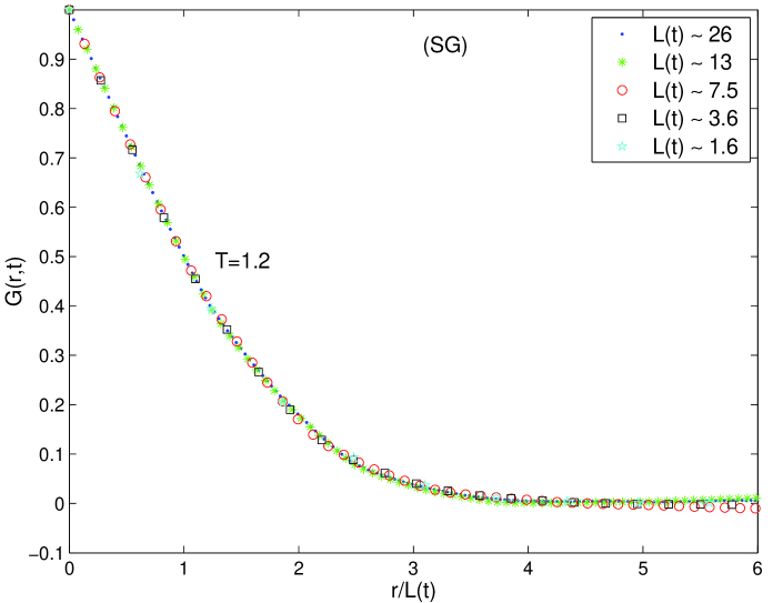
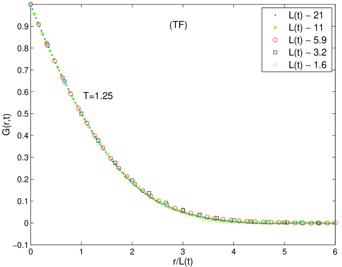
Figure 2: $G^{ag}(r,t)$ is plotted against $x=r/L(t)$ for the (TF) and the (SG), the time $t$ ranges from $10$ steps for the shortest $L(t)$ to $400000$ for the longest lengths.

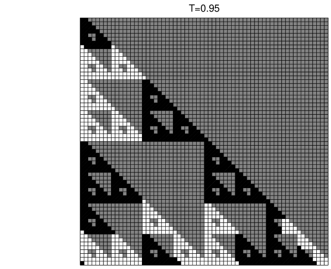
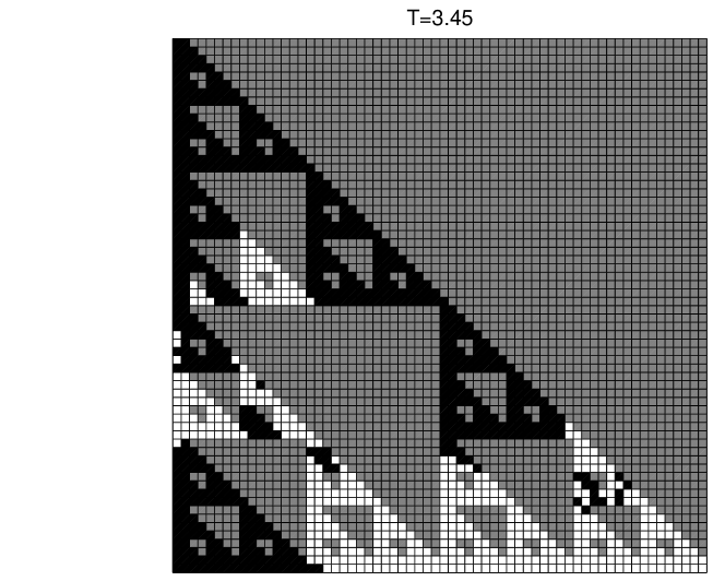
Figure 3: (SG) Two spin configurations after $t=1000$ step for the temperatures $T_{f}=0.95$ and $T_{f}=3.45$.

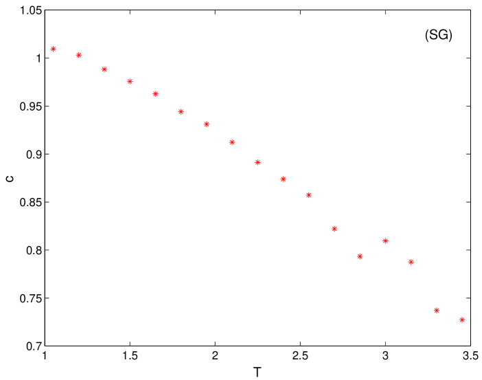
Figure 4: (SG) The exponent $c$ characterizing the behaviour of $g(x)$ for $x\simeq 0$.

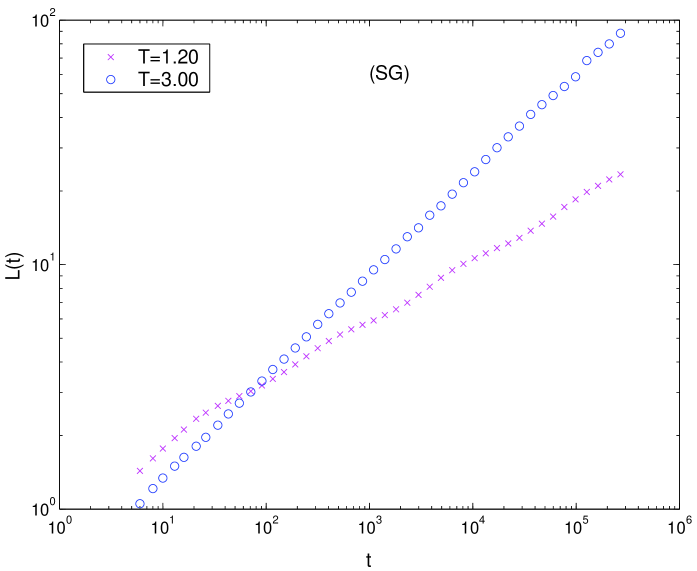
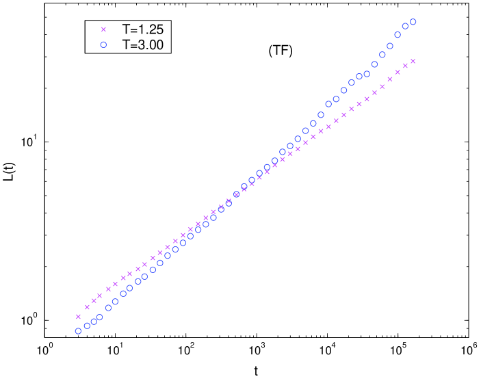
Figure 5: The characteristic length $L(t)$ is plotted against $t$, for two different temperatures $T_{f}=1.2$ and $T_{f}=3.0$ for the (SC) and $T_{f}=1.25$ and $T_{f}=3.0$ for the (TF).

The characteristic size $L(t)$, obtained as in Eq. (11), is shown in Fig. 5. This length grows roughly as a power law, but with a superimposed oscillation which is more pronounced at low temperatures. The origin of such oscillation, which is very reminiscent of what one observes in the related problem of Brownian motion on this structure woess , are again the pinning forces. In fact, as shown schematically in Fig. 6 for the SG, if two triangles happen to be ordered differently, in order to start reversing one of the two to achieve a global ordering, one has to flip one of the interfacial spins, for example the one marked with an arrow. This move requires an activation energy $\Delta E=4J$ and can then be accomplished on a time $\tau\simeq\exp(4J/T_{f})$. The dynamics then proceeds without activated processes until all the triangle is reversed but, then, a new activated step is required and so on. During the time $\tau$ the dynamics on the triangle in consideration is frozen. Since all the triangles have the same qualitative behavior, with some fluctuations, the overall behavior of $L(t)$ shows a periodic oscillation due to the recurring slow down caused by activated processes. An analogous phenomenon occurs in the TF. Clearly, since $\tau$ decreases at larger temperatures, this phenomenon is less evident, although still present even at relatively high temperatures, as shown on Fig. 5.

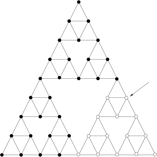
Figure 6: Schematic representation of a part of the structure, showing the necessity of activated processes.

The curves of Fig. 5 can be quite convincingly fitted by a power law with periodic oscillations superimposed. The exponent $z$ of the power law, however, should be thought as an effective exponent resulting from the balance between non activated processes obeying a growth law (8) with a certain value of $z$, and the activated processes whose net effect is an overall slowing down. Since the relative importance of these two processes is regulated by $T_{f}$, $z$ turns out to be temperature dependent, as shown in Fig. 7. On the basis of the previous discussion, one would expect to have a faster growth, namely a larger $1/z$, for higher $T_{f}$. This is indeed observed in Fig. 7 in a broad range. For very large temperatures $1/z$ seems to saturate. This is perhaps due to the neighborhood of the critical temperature (that with NBF turns out to be $T_{c}\simeq 3.6$ and $T_{c}\simeq 2$ for the SG and the TF, respectively), slowing down the dynamics much in the same way as it happens on regular lattices.

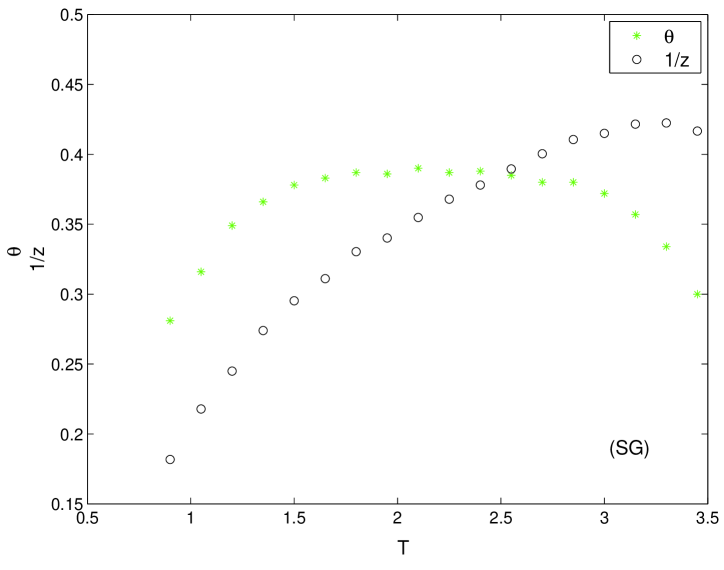
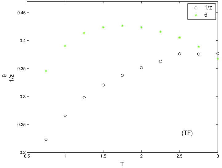
Figure 7: The dependence on temperature of the exponents $1/z$ and $\theta$ for the (SG) and the (TF).

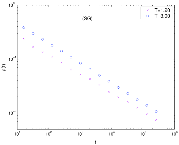
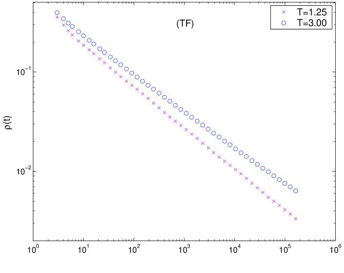
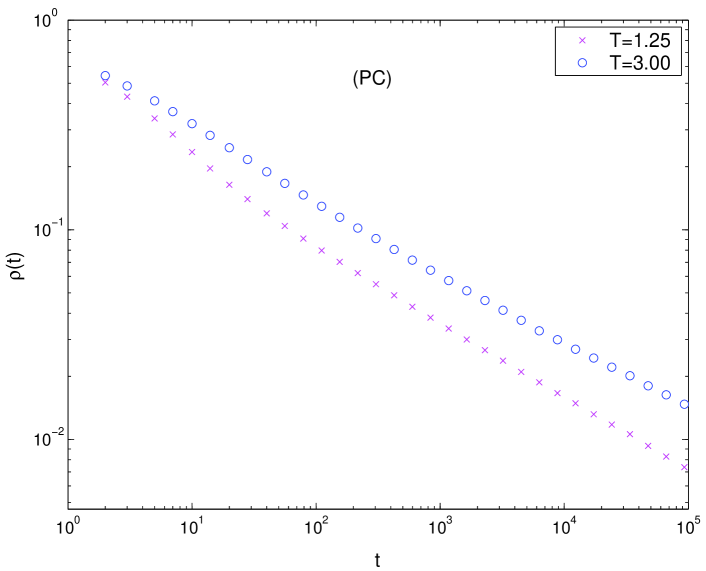
Figure 8: The density of interfaces $\rho(t)$ is plotted against $t$, at the temperatures $T_{f}=1.2$ and $T_{f}=3.0$ for the (SG), at $T_{f}=1.25$ and $T_{f}=3.0$ for the (TF) and (PC).

A pattern similar to that of $L(t)$ is observed for $\rho(t)$. This quantity, defined as the density of spin which are not fully aligned with their neighbors, is shown in Fig. 8 for the SG, TF and PC. Also in this case one observes oscillations on top of the power law behavior (12). The value of $\theta$ also depends on temperature, as shown in Fig. 7. Differently from $1/z$, however, the behavior is strongly non monotonous, with a broad maximum at intermediate temperatures. As already observed, the exponent $\theta$ and $1/z$ are not trivially related, as on homogeneous structures. In the limit of low temperatures one finds an exponent $\theta$ consistent with $\theta=-d_{f}/z$, which can be understood on the basis of the following argument. Let us consider again, for simplicity, the SG of Fig. 6. When the temperature is very low interfaces are very likely located in the pinning positions, as can be seen in Fig. 3. A domain, therefore, is a triangle of size $L(t)$, with a volume $V\propto L(t)^{d_{f}}$ and a number of surface spins $n_{s}=3$. The density of interfacial spins is, therefore $\rho(t)\sim L(t)^{-d_{f}}$. One then has

$$\theta=-\frac{d_{f}}{z},$$ (23)

instead of Eq. (13), holding on regular lattices. Let us remark again, however, that, although this relation is consistent with our data in the limit of small $T_{f}$, it is not of general validity. Actually, as already evident from Fig. 3 and from the non linear behavior of $g(x)$ at small $x$, for larger temperatures, interfaces are no longer located on the pinning centers.

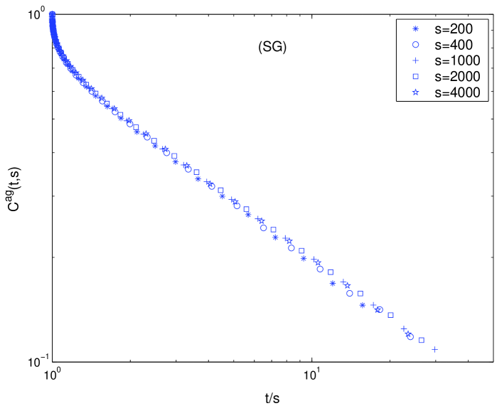
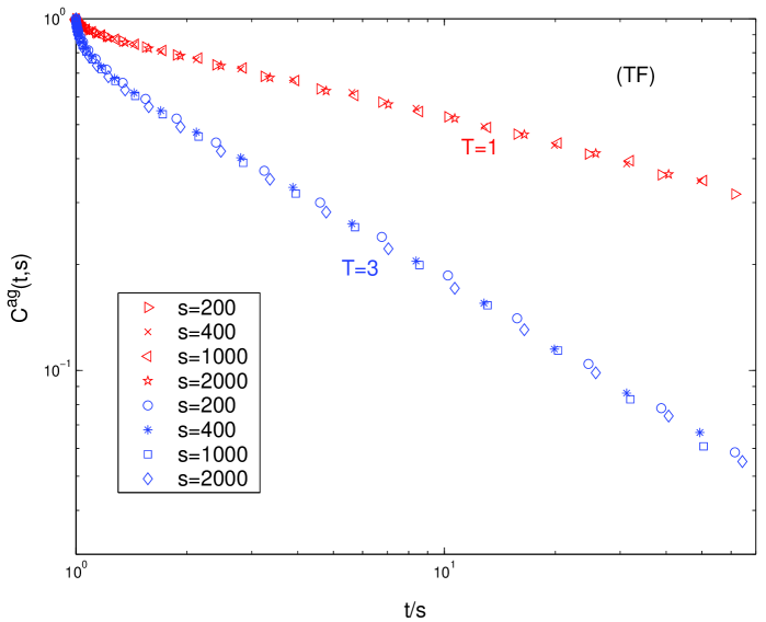
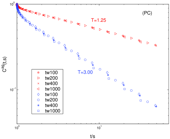
Figure 9: (SG) $C^{ag}(t,s)$ is plotted against $y=t/s$, at $T_{f}=3.0$ for the (SG), at $T_{f}=3.0$ and $T_{f}=1.0$ for the (TF) and at $T_{f}=3.00$ and $T_{f}=1.25$ for the (PC).

Let us consider now the behavior of two time quantities. The autocorrelation function for the SG, TF and PC are plotted in Fig. 9 against $y=t/s$. According to Eq. (17), one should observe data collapse of the curves with different $s$. This is indeed observed. One also finds the large-$y$ power law behavior (19) with an exponent $\lambda$ strongly dependent on temperature.

Let us turn to consider the response function. According to Eq. (18) the exponent $a_{\chi}$ can be obtained as the slope of a double logarithmic plot of $\chi^{ag}(t,s)$ against $s$, with $y$ held fixed. Such determination should be independent on $y$, within errors. We show this plot in Fig. 10 for the TF.

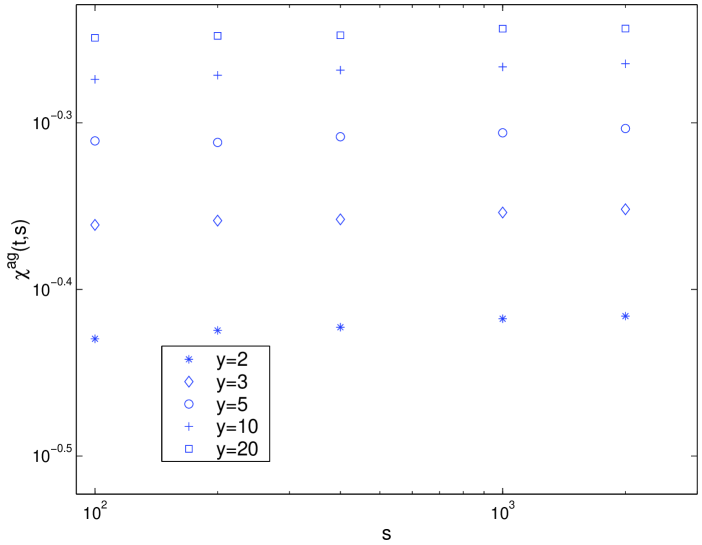
Figure 10: (TF) $\chi^{ag}(t,s)$ is plotted against $s$ for fixed values of $y=t/s$, for $T_{f}=3.00$.

We obtain $a_{\chi}=.01\pm.02$ which is consistent with $a_{\chi}=0$, similarly to what found in homogeneous systems with $T_{c}=0$ Lippiello00 ; Godreche00 ; Castellano04 . Analogous values are found for all the structures with $T_{c}=0$. Then, by plotting $\chi^{ag}(t,s)$ against $y$ one should find data collapse, how it is indeed shown in Fig. 11 for SG, TF and PC at different temperatures.

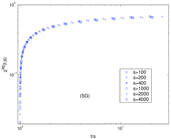
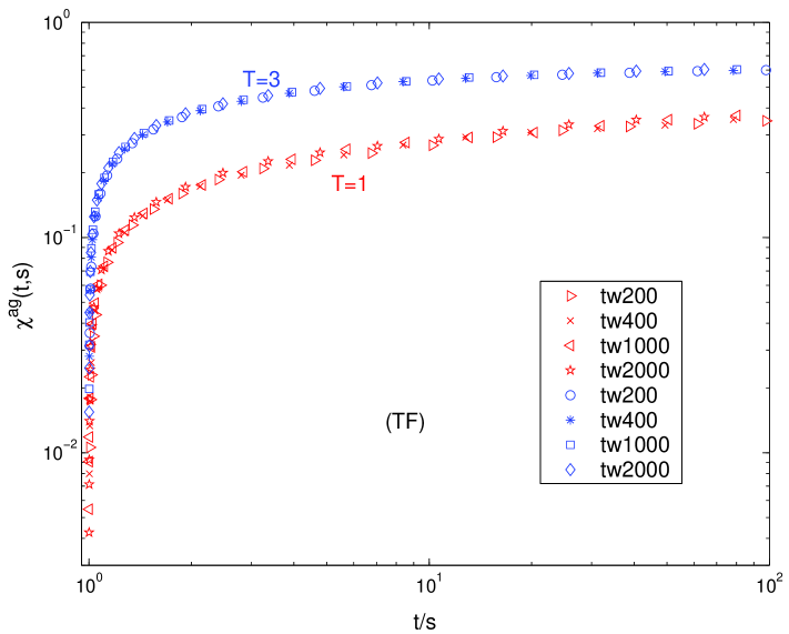
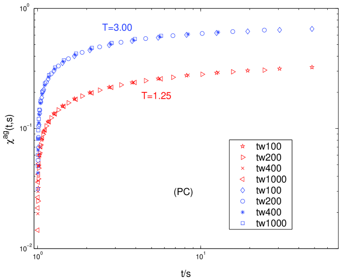
Figure 11: (SG) $\chi^{ag}(t,s)$ is plotted against $y=t/s$ for different values of $s$, for $T_{f}=3.00$ (SG), $T_{f}=3.00$ and $T_{f}=1.00$ (TF) and for $T_{f}=3.00$ and $T_{f}=1.25$ (PC).

III.2 Graphs with $T_{c}>0$

In this Section we will consider systems of class I. In particular we will study the phase-ordering kinetics on the diluted square lattice (DS) above the percolation threshold, the toblerone lattice (TL) obtained by replicating the Sierpinski gasket along a third spatial direction $z$, and the Sierpinski carpet (SC). These structures are represented in Fig. 1.

For the SC, we have computed the equal time correlation function (9) along the borders of the structure, analogously to what done for the SG. The TL is an anisotropic structure, since it is translational invariant along the $z$ direction alone. Therefore we have computed the equal time correlation function on the planes with a constant $z$, and in the $z$ direction separately. These are denoted as $G^{ag}_{xy}(r,t)$ and $G^{ag}_{z}(r,t)$, respectively. The former is computed along the borders of the structure, as for the SG. In Fig. 12 $G^{ag}(r,t)$ is plotted against $x=r/L(t)$ for the TL and the SC. One finds a very good data collapse for the TL, as expected on the basis of Eq. (10). The scaling is less accurate for the SG, where the pinning effects seem to be stronger. Notice also in these cases, the presence of the Porod’s tail, for small $x$, implying that interfaces are sharp objects at low temperature. As in the case of the SG, when the temperature is raised the interfaces broaden and the Porod behavior does not longer hold.

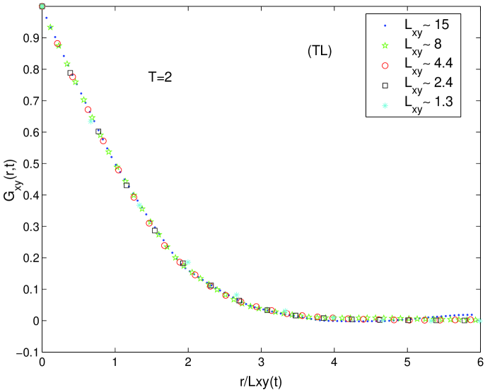
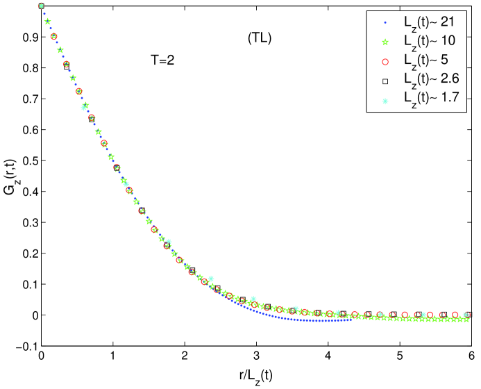
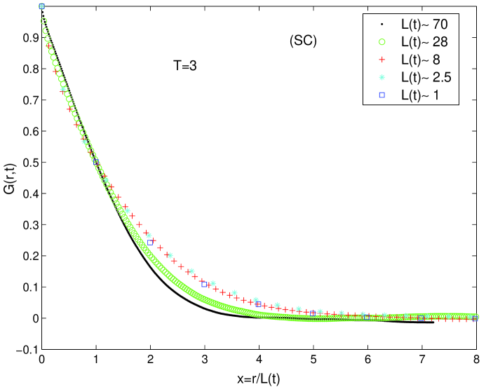
Figure 12: For the (TL) we plotted $G^{ag}_{xy}(r,t)$ and $G^{ag}_{z}(r,t)$ against $x=r/L(t)$ for the (SC) we plotted $G^{ag}(r,t)$.

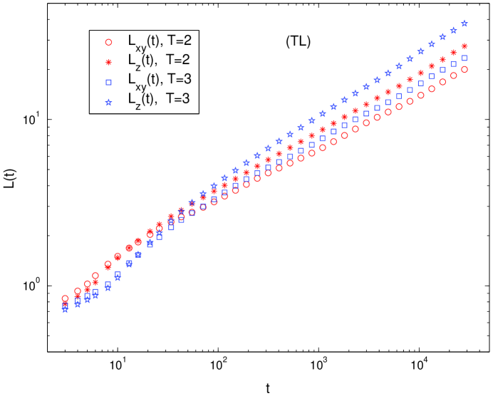
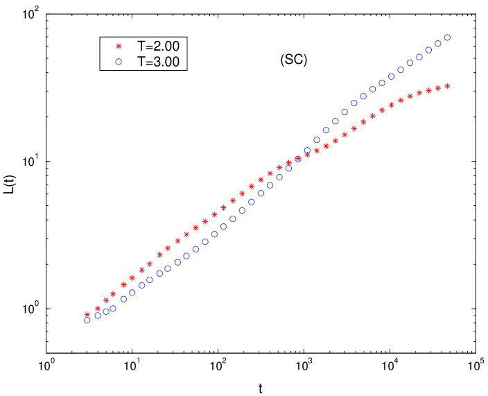
Figure 13: For the TL The characteristic lengths $L_{xy}(t)$ and $L_{z}(t)$ are plotted at the temperatures $T_{f}=2.0$ and $T_{f}=3.0$. For the (SC) $L(t)$ is plotted against $t$, at $T_{f}=2.0$ and $T_{f}=3.0$.

The characteristic size $L(t)$, obtained as in Eq. (11), is shown in Fig. 13. For the TL there are two different lengths $L_{xy}(t)$ and $L_{z}(t)$ obtained from $G^{ag}_{xy}(r,t)$ and $G^{ag}_{z}(r,t)$ respectively. Note also in this case the presence of oscillations on top of an average power-law growth, as discussed in Sec. III.1. For the SC the exponent $z$ is $z\simeq 0.33$ and $z\simeq 0.45$ at $T_{f}=2.00$ and $T_{f}=3.00$. The behavior of $\rho(t)$ is similar to that found for the structures with $T_{c}=0$, discussed in Sec. III.1. This quantity, is shown in Fig. 14 for the DS, TL and SC. For the SC, $\theta\simeq 0.38$ and $\theta\simeq 0.43$ at $T_{f}=2.0$ and $T_{f}=3.0$. Therefore also on these structures both $\theta$ and $z$ depends on the temperature.

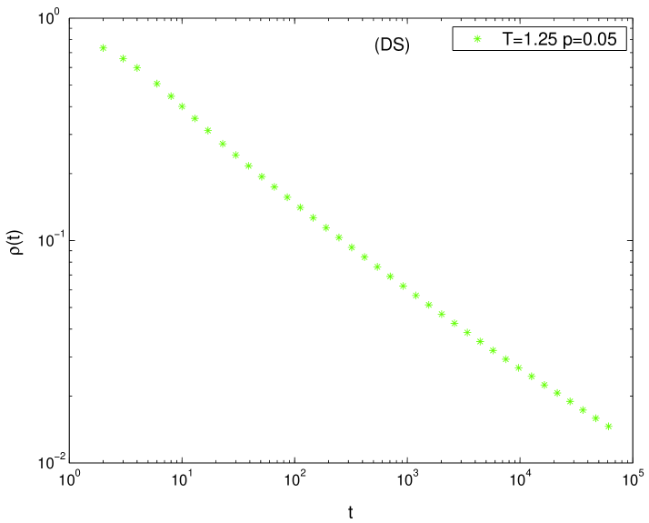
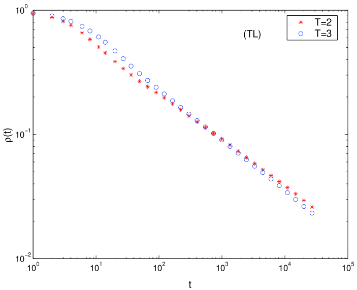
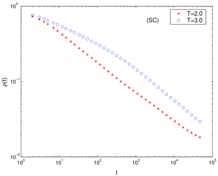
Figure 14: (DS) The density of interfaces $\rho(t)$ is plotted against $t$, at the temperature $T_{f}=1.25$ for the (DS), at $T_{f}=2.00$ and $T_{f}=3.00$ for the (TL) and for the (SC).

Let us consider now the behavior of two time quantities. The autocorrelation function for the DS, TL and SC are plotted in Fig. 15 against $y=t/s$.

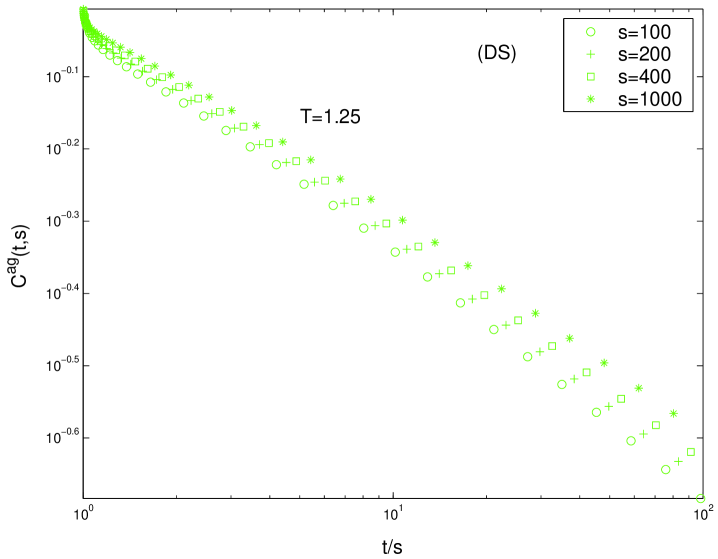
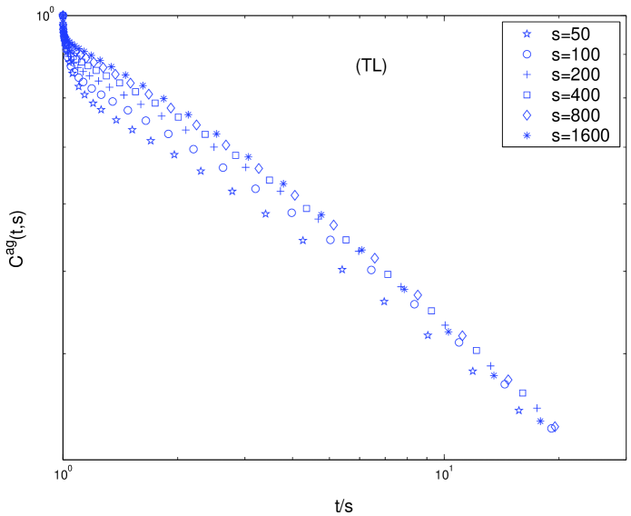
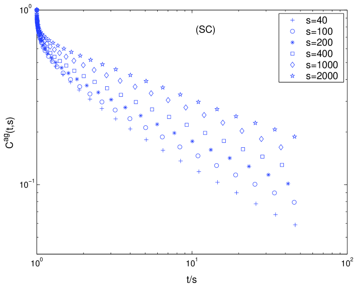
Figure 15: (DS) $C^{ag}(t,s)$ is plotted against $y=t/s$, at $T_{f}=1.25$ for the (DS) and at $T_{f}=3.00$ for the (TL) and (SC).

For the TL one has a good data collapse for the larger values of $s$, according to Eq. (17). The situation is different for the DS and SC. In these cases, there is no data collapse in the range of time accessed in our simulations. Probably this is due to preasymptotic effects and larger values of $s$ then those presented in the figure should be needed to obtain the scaling of Eq. (17).

Let us turn to consider the response function. From $\chi^{ag}(t,s)$ we extract $a_{\chi}$ as the slope of a double logarithmic plot of $\chi^{ag}(t,s)$ against $s$, with $y$ held fixed, as described regarding Fig. 10.

We obtain $a_{\chi}=0.21$, $a_{\chi}=0.25$ and $a_{\chi}=0.18$ for the DS, the TL and the SC, respectively. Plotting $s^{a_{\chi}}\chi^{ag}(t,s)$ against $y$ we find a good data collapse, independently from the temperature, as shown in Fig. 16, indicating that Eq. (18) is obeyed. Also the large-$y$ behavior (20) is obeyed.

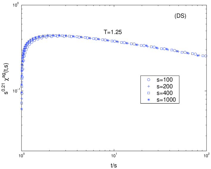
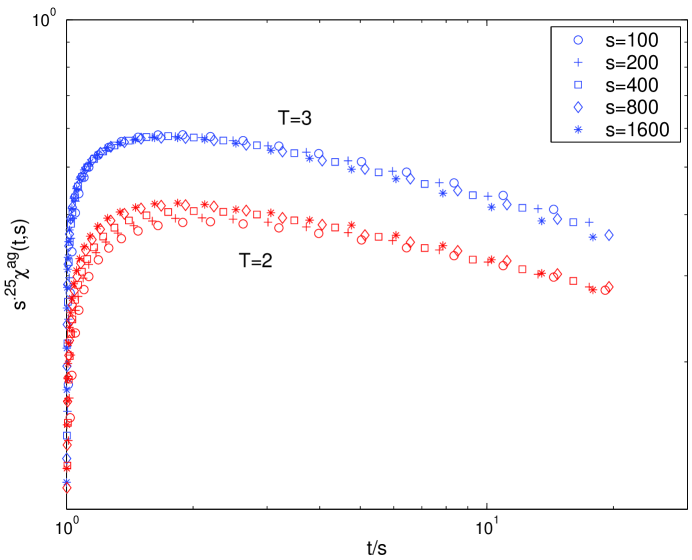
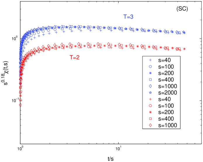
Figure 16: $\chi^{ag}(t,s)$ is plotted against $y=t/s$ for different values of $s$, at $T_{f}=1.25$ for the (DS), at $T_{f}=2.00$ and $T_{f}=3.00$ for the (TL) and the (SC).

IV The response function exponent and the fluctuation dissipation plot

In the previous Section, we have checked the validity of the scaling form (18) in the fractal structures considered, and we have determined the value of the exponent $a_{\chi}$. As already emphasized, while all the other quantities turn out to be very sensitive to the final temperature of the quench, this exponent assumes a well defined value in all the low temperature region. On regular lattices, analytical calculations in the vector ${\cal O}({\cal N})$ model in large-${\cal N}$ limit ninf find the following dependence on dimensionality

$$a_{\chi}=\left\{\begin{array}[]{ll}\theta\frac{d-d_{L}}{d_{U}-d_{L}}\qquad$for$\qquad d<d_{U}\\ \theta\qquad$with log corrections for$\qquad d=d_{U}\\ \theta\qquad$for$\qquad d>d_{U},\end{array}\right.$$ (24)

where $d_{L}$ is the lower critical dimension of static critical phenomena and $d_{U}=4$. Numerical simulations altri1 ; altri2 ; Castellano04 of discrete and ${\cal O}({\cal N})$ vectorial systems, with conserved and non conserved order parameter, are consistent with Eq. (24), and $d_{U}=3$ or $d_{U}=4$ for scalar or vectorial models respectively. This shows that the non-equilibrium exponent, $a_{\chi}$, is related in a non-trivial way to the topology of the underlying lattice, through $d$. Interestingly, this relation implies $a_{\chi}>0$ when the system is above $d_{L}$, i.e. when a phase transition at finite temperature $T_{c}$ is present, $a_{\chi}=0$ at $d_{L}$ and $a_{\chi}<0$ below $d_{L}$. This result for regular lattices suggests that the non-equilibrium dynamics of statistical models, and in particular the response function exponent, could be related to important topological properties also in the case of generic graphs. This hypothesis can be checked in some detail in systems with a continuous symmetry, because in this case it is well known that a large scale parameter, the ”spectral dimension” $d_{s}$, encodes the relevant topological features, uniquely determines the existence of phase transitions fss and controls the critical behavior sferico . In other words on generic networks $d_{s}$ plays the same role played by the Euclidean dimension $d$ on regular lattices. In particular, vectorial models on graphs exhibit a phase transition at finite temperature only if $d_{s}>d_{L}=2$. Solving an ${\cal O}({\cal N})$ model in the large-${\cal N}$ limit prlnostro one can show that this property holds true also for the non-equilibrium exponent $a_{\chi}$. In fact, one finds the same expression (24) as for regular lattices, with $d_{s}$ replacing $d$. Then, again one has $a_{\chi}>0$ when the system is above $d_{L}$, i.e. when a phase transition at finite temperature $T_{c}$ is present, and $a_{\chi}\leq 0$ when $T_{c}=0$ prlnostro . The conclusion is that, for models with a continuous symmetry there is a well defined relation between the non equilibrium exponent $a_{\chi}$ and the topological features of the network which regulate the critical properties. In this case, this features are totally described by a single index, namely $d_{s}$. The next question is if a similar picture hold for scalar systems, where the counterpart of $d_{s}$ is not known. Namely, if the non equilibrium exponent $a_{\chi}$ is related to the critical properties, and in turn to topology, such that $a_{\chi}>0$ or $a_{\chi}\leq 0$ holds for graphs with $T_{c}>0$ or $T_{c}=0$ respectively. An argument prlnostro based on the topology of class II networks suggests that $a_{\chi}=0$ is expected for these systems. The values of $a_{\chi}$ reported in the previous Section III show quite convincingly that the above conjecture is verified in all the cases considered in our simulations. One has $a_{\chi}\simeq 0$ in all the structures of class II and $a_{\chi}>0$ in those of class I. This result is particularly interesting for discrete symmetry models. In fact, while for ${\cal O}({\cal N})$ models the presence of phase transition can be inferred from $d_{s}$, there is not a such a general criterion for discrete models. Our data suggest that $a_{\chi}$ may be used to infer the presence of phase transition on a generic network. We recall again that this result directly links $a_{\chi}$ to some relevant topological features of graphs. For this reason, although $a_{\chi}$ is a non-equilibrium dynamical exponent, it is totally independent on all the non-universal details of the dynamics we have described in Sec. III. We have already observed, in fact, that, differently from all the other dynamical exponent, its value is robust and temperature independent.

Finally, we mention that the value $a_{\chi}=0$ found in the structures of class II is associated to an anomalous fluctuation-dissipation plot altri1 . Re-parameterizing in $\chi(t,s)$ the time $t$ in terms of $C(t,s)$, according to the theorem by Franz, Mezard, Parisi and Peliti Franz98 , under broad hypoteses the following relation

$$-T_{f}\lim_{s\to\infty}\left.\frac{d^{2}\chi(C,s)}{dC^{2}}\right|_{C=q}=P_{eq}(q)$$ (25)

exists between the non equilibrium two time functions $\chi,C$ and the equilibrium probability distribution $P_{eq}(q)$ of the overlaps $Q([\sigma],[\sigma^{\prime}])=(1/N)\sum_{i=1}^{N}\sigma_{i}\sigma_{i}^{\prime}$ between two configurations $[\sigma],[\sigma^{\prime}]$

$$P_{eq}(q)=\frac{1}{Z^{2}}\sum_{[\sigma],[\sigma^{\prime}]}\exp\{-\beta(H[\sigma]+H[\sigma^{\prime}])\}\delta(Q([\sigma],[\sigma^{\prime}])-q).$$ (26)

Using the $\delta$-like form of $P_{eq}(q)$ of the low temperature state of the ferromagnetic models considered in this paper, one obtains altri1 the well known broken line fluctuation-dissipation plot of $\chi$ versus $C$. However, as discussed in prlnostro , when $a_{\chi}=0$ the theorem (25) cannot be applied and one gets a non-trivial fluctuation-dissipation plot which is not related to $P_{eq}(q)$.

V Discussion and conclusions

In this paper we have studied the phase-ordering kinetics of the Ising model with spin flip dynamics on a class of physical graphs. The evolution is in many respects qualitatively similar to what observed on regular lattices. After the quench one has the formation and growth of domains of the two competing ordered phases, and a scaling symmetry is obeyed quite generally (except for the SC in the timescale of our simulations). However, differently from coarsening on regular lattices, the fractal nature of the networks pins the interfaces on locally stable positions. Escape from the pinned positions is achieved by means of activated processes, but subsequently the interfaces are trapped again. When interfaces are pinned, the growth of the domain size $L(t)$ is inhibited. Because of this recurrent phenomenon the usual power growth-law of $L(t)$ is modulated by an oscillation, which is more evident when the pinning is stronger, namely at low temperatures. The necessity of activated moves on all time/space scales makes a great difference with respect to regular lattices. On regular lattices the temperature is an irrelevant parameter Bray94 , in the sense of the renormalization group. Namely, in all the low temperature region the dynamics is controlled by the zero temperature fixed point. One has, therefore, the same dynamical exponents in all quenches to $T_{f}<T_{c}$, regardless of the temperature. On fractal networks, instead, the situation is different, because the dynamics of activated processes are faster the higher is $T_{f}$. As a consequence, exponents are always found temperature dependent.

A notable exception is the response function exponent $a_{\chi}$, which turns out to be stable and temperature independent. This already suggests that $a_{\chi}$ may be related to a more fundamental property of the system which remains stable under temperature variations. Interestingly, we find $a_{\chi}=0$ on all the considered graphs which do not support a ferro-paramagnetic transition at a finite critical temperature, while $a_{\chi}>0$ in all the other cases. The same situation was found ninf ; altri1 ; altri2 on regular lattices, where $a_{\chi}$ is related to the euclidean dimension. On these lattices, the euclidean dimension is the topological parameter that determines the exhistence of phase transitions and regulates the critical properties. This calls for the hypoteses that, also on generic graphs, $a_{\chi}$ could be related to the relevant topological features which govern the critical behavior, although for systems with a discrete symmetry, such as the Ising model considered here, a unique topological indicator, analogous to $d$ is not known. Interestingly, this fact suggests that $a_{\chi}$ can be used to infer topological properties of graphs.

Acknowledgments - This work has been partially supported from MURST through PRIN-2004.

References

- (1) A.J. Bray, Adv.Phys. 43, 357 (1994).
- (2) H. Furukawa, J.Stat.Soc.Jpn. 58, 216 (1989); Phys.Rev. B 40, 2341 (1989).
- (3) D.A.Beysens, G. Forgacs, J.A. Glazier, Proc. Nat. Ac. Sci. 97, 9467 (2000); C. Castellano. M. Marsili, A. Vespignani, Phys. Rev. Lett. 85 3536 (2000).
- (4) R.Burioni, D.Cassi, Jour. Phys. A 38 R45 (2005).
- (5) U. Marini Bettolo Marconi, A. Petri, Phys. Rev. E 55, 1311 (1997).
- (6) R. Burioni, D. Cassi, F. Corberi, A. Vezzani Phys. Rev. Lett. 96 235701 (2006).
- (7) U. Marini Bettolo Marconi, Phys.Rev.E 57, 1290 (1998).
- (8) Y.Gefen, A.Aharony and B.B.Mandelbrot, Jour. Phys. A 16 1267 (1983); Y.Gefen, A.Aharony, Y. Shapir and B.B.Mandelbrot, Jour. Phys. A 17 435 (1984).
- (9) F. Corberi, E. Lippiello and M. Zannetti, Phys.Rev.E 72, 056103 (2005).
- (10) M.J. de Oliveira, J.F.F. Mendes and M.A. Santos, J.Phys.A 26, 2317 (1993). J.M. Drouffe and C. Godrèche, J.Phys.A 32, 249 (1999).
- (11) F. Liu and G.F. Mazenko, Phys.Rev.B 47, 2866 (1993).
- (12) C. Chatelain, J.Phys.A 36, 10739 (2003).
- (13) F. Ricci-Tersenghi, Phys.Rev.E 68, 065104(R) (2003).
- (14) E. Lippiello, F. Corberi, and M. Zannetti, Phys.Rev.E 71, 036104 (2005). Other methods for measuring the response function without applying the perturbation have been introduced in Chatelain03 ; Ricci03 .
- (15) P. J. Grabner and W. Woess, Stochastic Process. Appl. 69 (1997).
- (16) E.Lippiello and M.Zannetti, Phys.Rev.E 61, 3369 (2000).
- (17) C.Godrèche and J.M.Luck, J.Phys. A 33, 1151 (2000)
- (18) F. Corberi, C. Castellano, E. Lippiello and M. Zannetti, Phys.Rev. E 70, 017103 (2004).
- (19) F. Corberi, E. Lippiello and M. Zannetti, Phys.Rev. E 65, 046136 (2002).
- (20) F. Corberi, E. Lippiello and M. Zannetti, Phys. Rev. E 63, 061506 (2001); Eur.Phys.J.B 24, 359 (2001).
- (21) F. Corberi, E. Lippiello and M. Zannetti, Phys.Rev.Lett. 90, 099601 (2003); Phys.Rev. E 68, 046131 (2003).
- (22) R.Burioni, D.Cassi, and A.Vezzani, Phys. Rev. E 60 1500 (1999).
- (23) R. Burioni, D. Cassi, and C. Destri, Phys. Rev. Lett. 85 1496 (2000).
- (24) S.Franz, M.Mézard, G.Parisi and L.Peliti, Phys. Rev. Lett. 81, 1758 (1998); J.Stat.Phys. 97, 459 (1999).