Hole dynamics in an antiferromagnet
across a deconfined quantum critical point

Abstract

We study the effects of a small density of holes, $\delta$, on a square lattice antiferromagnet undergoing a continuous transition from a Néel state to a valence bond solid at a deconfined quantum critical point. We argue that at non-zero $\delta$, it is likely that the critical point broadens into a non-Fermi liquid ‘holon metal’ phase with fractionalized excitations. The holon metal phase is flanked on both sides by Fermi liquid states with Fermi surfaces enclosing the usual Luttinger area. However the electronic quasiparticles carry distinct quantum numbers in the two Fermi liquid phases, and consequently the ratio $\lim_{\delta\rightarrow 0}\mathcal{A}_{F}/\delta$ (where $\mathcal{A}_{F}$ is the area of a hole pocket) has a factor of 2 discontinuity across the quantum critical point of the insulator. We demonstrate that the electronic spectrum at this transition is described by the ‘boundary’ critical theory of an impurity coupled to a 2+1 dimensional conformal field theory. We compute the finite temperature quantum-critical electronic spectra and show that they resemble “Fermi arc” spectra seen in recent photoemission experiments on the pseudogap phase of the cuprates.

I Introduction

There was a great deal of work on the dynamics of a single hole in a square lattice antiferromagnet, soon after the discovery of high temperature superconductivity in the cuprate compounds. It was demonstratedtrugman ; ssneel ; elser ; klr ; martinez ; poilblanc ; reiter ; mish that a single hole moving in a Néel ground state has a finite quasiparticle residue, $Z$; so a small density of holes, $\delta$, are expected to form a Fermi liquid. This Fermi liquid state with Néel order will be the starting point of our analysis. Also, Shraiman and Siggia ss ; wiese introducing a current-current coupling between the hole and the antiferromagnet which implied that a large spin $S$ Néel state is unstable for certain parameter ranges to spiral spin ordering; we shall not be interested in this metallic spiral state here, although the Shraiman-Siggia coupling (in Eq. (13) below) will play a key role in our analysis.

We begin with a $S=1/2$ Néel state of an insulating antiferromagnet and imagine “turning up quantum fluctuations” by adding further neighbor or ring-exchange couplings so that there is a transition to a paramagnetic state in which spin rotation invariance is restored. Now add a small density of holes to this antiferromagnet. The main question we shall address is: what is the fate of the Fermi liquid Néel state across such a transition ?

Specifically, we consider the ‘deconfined’ quantum phase transition proposed in Ref. senthil1, for an insulating $S=1/2$ square lattice antiferromagnetproko ; anders ; kamal ; mv . This is a theory for a transition between a Néel state and a spin-gap state with valence bond solid (VBS) order (the latter state is spin rotation invariant, but breaks lattice symmetries by ordering of valence bonds). These two states break distinct symmetries of the Hamiltonian, and so cannot generically have a continuous transition between them in the Landau-Ginzburg-Wilson theory of phase transitions. However, such a transition is found in a ‘deconfined’ theory focusing not on order parameters but on fractionalized excitations and emergent gauge forces. The transition is tuned by the coupling $s$ (which represents the strength of frustrating exchange interactions)—see Fig. 1.

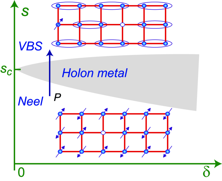
Figure 1: Schematic phase diagram. The ellipses represent spin singlet valence bonds. The coupling $s$ tunes the insulator across the Néel-VBS transition, and $\delta$ is the mobile hole density. The deconfined quantum critical point is at $s=s_{c}$ in the insulator with $\delta=0$. The vacancies (‘holons’) carry a gauge charge $q=\pm 1$ under an emergent U(1) gauge force. In the cartoons above, the reader can interpret $q$ as a sublattice label. In the $s<s_{c}$, Néel phase, $q$ determines the spin: a vacancy on an up (down) spin site carries net spin down (up) and so is equivalent to a charge $e$ spin-1/2 hole. For $s>s_{c}$, the hole is a composite of a vacancy and a nearby unpaired spin with opposite $q$, moving by rearranging nearest-neighbor valence bonds; note that this motion preserves spin and sublattice quantum numbers separately (see also Ref. ls, ). So there are twice as many states per momentum for a charge $e$ spin 1/2 hole in the VBS state than there are in the Néel state.

Upon doping, we will argue that the most likely possibility is that the insulating deconfined critical point gets broadened into a novel non-Fermi liquid ‘holon metal’ phase, with no Fermi surface (shown shaded in Fig. 1). The qualitative distinction between the Néel and VBS states survives also in the Fermi liquid states at $\delta>0$ (shown unshaded in Fig. 1): we will show that a characteristic property (specified shortly) of the Fermi surface has a discontinuity in the limit $\delta\rightarrow 0$ as $s$ is scanned across the $s=s_{c}$ critical point of the insulator. We also compute finite temperature electronic spectra in the vicinity of the transition and find that they resemble “Fermi arc” spectra seen in recent photoemission experiments on the pseudogap phase of the cupratesmohit .

There have been other discussions in the literaturecoleman0 ; qsi0 ; senthil0 of transitions between Fermi liquids, including proposals that there could be a continuous quantum transition with a discontinuous change in the shape of the Fermi surface (recent experiments onuki on CeRhIn₅ are compatible with an abrupt or very rapid change in Fermi surface topology). This would require a sudden change in the Fermi surface as a function of $s$ at a fixed non-zero value of $\delta$. We will argue that such a change is unlikely in our models, and the situation is as illustrated in Fig. 1, with an intermediate non-Fermi liquid phase.

By an extension of arguments in early work wensc ; palee ; shankar ; sarker , it is expected that a significant portion of the phase diagram in Fig. 1 is unstable at low temperatures to superconductivity. We defer consideration of such superconducting states to future work, and limit ourselves here to the normal states.

We now turn to a more detailed summary of our results. First, we discuss our results in the unshaded regions of Fig 1. In these regions, we are adding a small density of mobile carriers to conventionally ordered insulators, and we obtain Fermi liquid phases with electron-like quasiparticles with a non-zero quasiparticle residue, i.e. $Z\neq 0$. Non-Fermi-liquid physics appears only in the shaded region.

In the $s<s_{c}$ Néel phase, we obtain a Fermi liquid statetrugman ; ssneel ; elser ; klr ; martinez ; poilblanc ; reiter ; mish with four hole pockets centered at the $\vec{K}_{p}=(\pi/2a)(\pm 1,\pm 1)$, where $a$ is the lattice spacing, shown in Fig. 2.

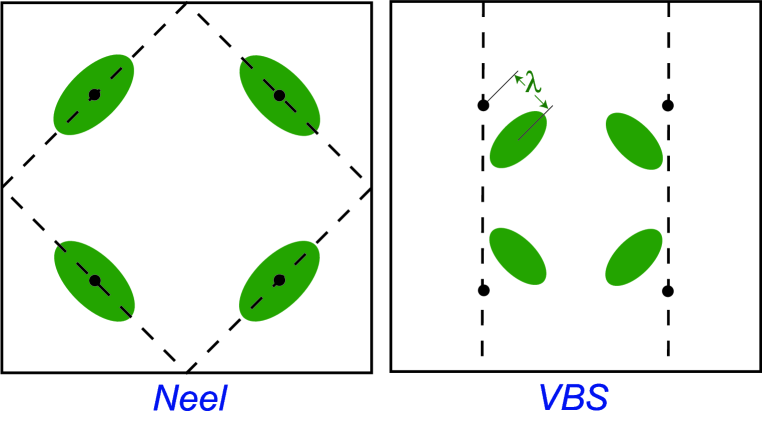
Figure 2: Momentum space Fermi surfaces in the Néel and VBS regions of Fig 1. The filled circles are the 4 $\vec{K}_{p}$ wavevectors, with $\vec{K}_{1}=(\pi/2a)(1,1)$, $\vec{K}_{2}=(\pi/2a)(1,-1)$, $\vec{K}_{3}=-\vec{K}_{1}$, $\vec{K}_{4}=-\vec{K}_{2}$, with $a$ the lattice spacing. The dashed line in the Néel phase indicates the boundary of the magnetic Brillouin zone. Only the Fermi surfaces within this zone contribute to the Luttinger counting, and so the area of each ellipse is $\mathcal{A}_{F}=(2\pi)^{2}\delta/4$. In the VBS phase, all 4 pockets are inequivalent, and so the area of each ellipse is $\mathcal{A}_{F}=(2\pi)^{2}\delta/8$. The dashed lines now show the reduction of the Brillouin zone due to the VBS order which appears at sufficiently low temperatures; “shadow” Fermi sufaces, with weak photoemission intensity (estimated in the text), will appear as reflections across these lines, and these Fermi surfaces are not shown.

However, because of the halving of the Brillouin zone by magnetic order, only two of these pockets are distinct. After accounting for the two-fold spin degeneracy, we conclude that the area enclosed by each pocket is $\mathcal{A}_{F}=(2\pi)^{2}\delta/4$. Another way of understanding this halving of the Brillouin zone (which is also indicated in the caption of Fig. 1, and discussed further in Section III) is as follows. We can consider the doped hole as a vacancy in the background of a Néel state. If this hole is to move without leaving a string of broken bondstrugman , it must preserve its sublattice label. However, because of the broken symmetry associated with the Néel order, the sublattice location is not independent of the spin of the vacancy, and two labels are really the same quantum number.

Next, we discuss a small density of holes in the $s>s_{c}$ VBS state. As we will demonstrate in Section IV, in this state the four hole pockets are no longer pinned at the $\vec{K}_{p}$, but instead move a distance $\lambda$ away, as indicated in Fig. 2. This shift arises from the Shraiman-Siggia ss coupling. The value of $\lambda$ is determined by $s-s_{c}$, but is independent of $\delta$ to lowest order in $\delta$. Consequently, for sufficiently small $\delta$, the hole pockets do not intersect the reduced Brillouin zone boundaries, associated with the appearance of VBS order. The four hole pockets therefore all contain distinct quasiparticles states, and after accounting for the two-fold spin degeneracy, we now conclude that the area enclosed by each pocket is $\mathcal{A}_{F}=(2\pi)^{2}\delta/8$. As above, another interpretation of this result is indicated in Fig 1, and will be described in more detail in Section IV: the hole motion in the VBS state also preserves its sublattice index, but now the sublattice and spin labels are distinct quantum numbers.

We can summarize the above statements into one of the main zero temperature results of this paper:

$$\lim_{\delta\rightarrow 0}\left.\frac{\mathcal{A}_{F}}{\delta}\right|_{s<s_{c}}=2\times\lim_{\delta\rightarrow 0}\left.\frac{\mathcal{A}_{F}}{\delta}\right|_{s>s_{c}}$$ (1)

Note that on both sides of the equation, we are taking the limit $\delta\rightarrow 0$ at fixed $s$. Thus, although a characteristic feature of the Fermi surface (the ratio $\mathcal{A}_{F}/\delta$) changes discontinuously as $s$ crosses $s_{c}$, the Fermi surface itself is of vanishingly small size. The result in Eq. (1) does not constitute a discontinuous change in the Fermi surface in the sense of other proposalscoleman0 ; qsi0 ; senthil0 .

Next, we address the evolution of the Fermi surface along the fixed $\delta>0$ line $P$ in Fig 1. Aspects of the physics will be addressed in Section V, and some questions are deferred to future work. The key issue is the fate of the monopoles in the U(1) gauge theory which describes the deconfined critical point of the insulator at $s=s_{c}$. The situation has been discussed at length elsewhere senthil1 for $\delta=0$: the monopoles are irrelevant at the $s=s_{c}$ critical point, but are relevant for all $s>s_{c}$ where they induce confinement and VBS order. There are two distinct interesting possibilities for the fate of this transition for $\delta>0$ (a first-order transitions is, of course, also possible):
(i) The critical point at $s=s_{c}$, $\delta=0$ extends into a single line of deconfined critical points for $\delta=0$, with Fermi-liquid physics on either side of the line. In this case, physics discussed above Eq. (1) will apply also for $\delta>0$, and there will be a discontinuous Fermi surface change across a continuous transition, realizing scenarios postulated in previous work coleman0 ; qsi0 ; senthil0 . However, we will argue in Section V that this possibility is unlikely in the present model.
(ii) The deconfined critical point at $s=s_{c}$, $\delta=0$ broadens into a deconfined phase, extending over a finite range of $s$ values (shown as the shaded region in Fig. 1), with novel non-Fermi-liquid physics. The monopoles, which were suppressed by the gapless critical modes at the single point $s=s_{c}$ in the $\delta=0$ insulator, are now suppressed hermele over a finite range of values of $s$ by the additional gapless excitations associated with mobile charge carriers for $\delta>0$. Arguments supporting this possibility will appear in Section V. For reasons which will become clear in Section V, we will refer to this phase as a ‘holon metal’. This holon metal phase has no electron-like Fermi surfaces, and hence $Z=0$.

It is convenient to think about the phase diagram in the $s$-$\mu$ plane where $\mu$ is the chemical potential. For a range of $\mu$ in the Mott insulator the ground state does not change for fixed $s$. The point $s=s_{c}$ in this Mott insulator is the deconfined quantum critical point and its low energy theory is a conformal field theory (CFT). Below some critical $\mu_{c}$ the hole density $\delta$ holes will increase from zero as some power of $\mu-\mu_{c}$. It should be clear that the critical point at $s=s_{c}$, $\mu=\mu_{c}$ is an unstable multicritical point which controls the properties of the holon metal phase at low doping. In this perspectivevojta , we view $\mu_{c}-\mu$ as a relevant perturbation to the field theory describing this multicritical point. So at an energy, temperatures, or wavevectors higher than a low energy scale determined by $\delta$, the physics is described by the response of the CFT of the deconfined critical point of the Mott insulator to an infinitesimal hole density. We will argue in Section V that this response is associated with a ‘boundary CFT’ describing a quantum impurity in the bulk, 2+1 dimensional CFT. The result in Eq. (1) describing the Fermi liquid phases outside the shaded region of Fig. 1 can also be viewed as a consequence of the structure of this boundary CFT.

Section V.1 will explore practical consequences of the boundary CFT by presenting numerical results on the form of the finite temperature electronic spectral weight. This will be carried out using the full action presented in Section II, including terms that are formally corrections to scaling to the boundary CFT, but are important for experimental comparisons. We will find that the results resemble recent photoemission measurements on the pseudogap phase of the cupratesmohit ; in particular, the length of the “Fermi arcs” is roughly proportional to the temperature. Furthermore, we find that the Shraiman-Siggiass term, which was responsible for the shift in the centers of the hole pockets away from the $\vec{K}_{p}$ in the zero temperature VBS state (Section IV and Fig. 2), also shifts the centers of the finite temperature “Fermi arcs” from the $\vec{K}_{p}$, as is seen experimentally. This feature is not present in a recent theory based upon a ‘staggered-flux’ spin liquid arun .

We will begin in Section II by presenting the field theory which describes the CFT at $s=s_{c}$, $\delta=0$ and the perturbations which induce mobile carriers for $\delta>0$. The Fermi liquid phases of this field theory will be discussed in Sections III and IV for the Néel and VBS states respectively. The non-Fermi-liquid holon metal phase, and the finite temperature quantum criticality is described in Section V, and we conclude in Section VI.

II Field theory

There is a vast literature on the theory of the lightly doped antiferromagnet. Two main approaches have been taken. The ‘spin-fermion’ models chubukov , which are extrapolations of the weak-coupling Hartree-Fock theory of the Hubbard model, offer a convenient description of the Fermi liquid states with Néel order. However, these models cannot describe the transition to the VBS state, and so are not suitable for our purposes. The second approach, ss ; wiese departs from the spin-wave theory of the insulating antiferromagnet, and describes the coupling of the holes to a spin deformations of the antiferromagnet. In modern terms, this is formulated as ‘chiral perturbation theory’ in which the broken symmetry of the Néel state allows one to place constraints on the couplings between the mobile holes and the ‘chiral’ spin wave excitationswiese . However, the non-linear realization of the SU(2) spin rotation symmetry in the Néel state makes this approach cumbersome. For our purposes, a central shortcoming is that this approach is not able to describe the fermion spectrum in a state in which SU(2) symmetry is restored and the magnetic Brillouin zone expands to the full Brillouin zone of the square lattice: Bloch reflections across the magnetic Brillouin zone boundary do not disappear at any order in chiral perturbation theory. It is essential to considerations of Fermi surface topology that such effects are properly accounted for.

We will instead use a method in which the spin SU(2) symmetry is linearly realized and is kept explicit at all stages. We also want to explicitly preserve the full space group symmetry of the square lattice. In the insulator, this requires starting from a ‘spin liquid’ state. Although there is no gapped spin liquid insulator in Fig 1, the VBS state descends rs ; senthil1 from an instability of a particular U(1) spin liquid, aa and the latter will serve as our starting point. Also, the CFT at $s=s_{c}$, $\delta=0$, defines an ‘algebraic spin liquid’, and this is obtained as a gapless critical point in the theory of the same U(1) spin liquid.

It has been emphasized by Wen wenpsg that an essential characteristic of any spin liquid is its PSG: the projective symmetries of the various fields under elements of the square lattice space group. Because the fields carry charges under a gauge group which characterizes the spin liquid, they need not be invariant under such transformations—they are only required to be invariant up to a gauge transformation, and this is sufficient to preserve square lattice symmetry in all observables. Here we will show how the PSG can be extended from the insulator to the doped state, where it also places crucial constraints on the low energy effective theory. Another PSG-based analysis of a doped Mott insulator is in Ref. vortexpsg, for case where the spin liquid has fermionic spinons. Here we focus on the vicinity of the Néel-VBS transition where, as we review below, the spinons are bosonic.

The motion of charge carriers doped into an insulating square-lattice quantum antiferromagnet is conventionally described by the “$t$-$J$” model,

$$H_{t-J}=-\sum_{i,j,\alpha}t_{ij}(c^{\alpha\dagger}_{i}c_{j\alpha}+{\rm h.c.})+\sum_{i,j}J_{ij}\vec{S}_{i}\cdot\vec{S}_{j}+\ldots\,,$$ (2)

where $c^{\alpha\dagger}_{i}$ creates an electron with spin $\alpha$ on the sites $i$ of a square lattice and $\vec{S}_{i}=\frac{1}{2}\sum_{\alpha\beta}c^{\alpha\dagger}_{i}\vec{\sigma}_{\alpha}^{\beta}c_{i\beta}$, with $\vec{\sigma}$ the Pauli matrices. In addition, the constraint $\sum_{\alpha}c^{\alpha\dagger}_{i}c_{i\alpha}\leq 1$ is enforced on each site, modeling the large local repulsion between the electrons. It is important to note that our results are more general than a particular $t$-$J$ model, and follow almost completely from symmetry considerations. The ellipses in Eq. (2) additional short-range couplings which preserve square lattice symmetry and spin rotation invariance. The coupling $s$ is some axis in this multidimensional parameter space which accesses both the Néel and spin liquid phases in the insulator.

We will analyze $H_{t-J}$ by choosing a representation of the electron operator which obeys the constraint on each site, and most conveniently accesses the U(1) spin liquid describing the Néel-VBS transition. This is achieved by introducing neutral Schwinger bosons to represent the spin degrees of freedom, and spinless fermionic holons which track the charge. Although this is not essential, we will use distinct representations on the two square sublattices because this simplifies the mean-field structure of the spin liquid solution. On one sublattice of the square lattice we write the electron operator, $c_{\alpha}$ as

$$c_{\alpha}=b_{\alpha}f^{\dagger}_{+}$$ (3)

where $b_{\alpha}$ are canonical Schwinger bosons and $f_{+}$ are canonical fermionic holons. The constraint on each site now becomes

$$f_{+}^{\dagger}f_{+}+b^{\alpha\dagger}b_{\alpha}=1\,.$$ (4)

On the other sublattice, we use bosons which transform as a conjugate respresentation

$$c_{\alpha}=\varepsilon_{\alpha\beta}\overline{b}^{\beta}f^{\dagger}_{-}$$ (5)

with a similar constraint. We define the antisymmetric tensor $\varepsilon_{\alpha\beta}$ by $\varepsilon_{\uparrow\downarrow}=1$ and $\varepsilon_{\alpha\beta}=\varepsilon^{\alpha\beta}$. Notice that the representations in Eq. (3,5) have a U(1) gauge redundancy. The structure of the mean-field theory described below instructs us to take the continuum limit so that the U(1) gauge charges of $b_{\alpha}$ and $f_{+}$ are $+1$, while those of the $\overline{b}^{\alpha}$ and $f_{-}$ are $-1$.

First, we recall the mean field theory aa of $H_{t-J}$ in the insulator in the above representation. Here we can ignore the holons $f_{\pm}$. The exchange interactions are quartic in the Schwinger boson operators, and we decouple these by a Hubbard-Stratanovich transformation. This yields the mean field Hamiltonian for the U(1) spin liquid

$$H_{J}=-Q\sum_{\langle ij\rangle}b_{i\alpha}\overline{b}_{j}^{\alpha}+\mbox{H.c.}+\lambda\sum_{i}b_{i}^{\alpha\dagger}b_{i\alpha}+\lambda\sum_{j}\overline{b}_{j\alpha}^{\dagger}\overline{b}_{j}^{\alpha},$$ (6)

where $i$ is restricted to be on one sublattice, and $j$ on the other, and $Q$, $\lambda$ are positive constants to be determined by solving the mean-field equations. Upon adding frustrating exchange couplings to $H_{J}$, the mean field parameters will vary, allowing us to access both the Néel and spin liquid phases. For sufficiently large $\lambda$, the boson spectrum is gapped, and this describes the spin liquid ($s>s_{c}$). As $\lambda$ is decreased, the bosons eventually condense, leading to a transition to the Néel state. We now want to obtain a continuum field-theoretic representation of this quantum phase transition of the insulator. This can done by carefully taking the continuum limit of the low energy excitations of $H_{J}$, and then including fluctuations about the mean-field saddle point: such a procedure is described in detail in Ref. rs, . Here, we show that the same answer can be rapidly obtained by a PSG analysis. For this, we need to understand how $H_{J}$ preserves the full square lattice symmetry even though it treats the two sublattices inequivalently. So we consider the transformations of the operators under all the space group operations of the square lattice, and also under time-reversal. These are listed in Table 1.

	$T_{x}$	$R_{\pi/2}^{\rm dual}$	$I_{x}^{\rm dual}$	$\mathcal{T}$
$~{}~{}b_{\alpha}$	$~{}\varepsilon_{\alpha\beta}\overline{b}^{\beta}~{}$	$~{}\varepsilon_{\alpha\beta}\overline{b}^{\beta}~{}$	$~{}\varepsilon_{\alpha\beta}\overline{b}^{\beta}~{}$	$~{}\varepsilon_{\alpha\beta}b^{\beta\dagger}~{}$
$\overline{b}^{\alpha}$	$\varepsilon^{\alpha\beta}{b}_{\beta}$	$\varepsilon^{\alpha\beta}{b}_{\beta}$	$\varepsilon^{\alpha\beta}{b}_{\beta}$	$\varepsilon^{\alpha\beta}\overline{b}_{\beta}^{\dagger}$
$f_{+}$	$f_{-}$	$f_{-}$	$f_{-}$	$f_{+}^{\dagger}$
$f_{-}$	$-f_{+}$	$-f_{+}$	$-f_{+}$	$f_{-}^{\dagger}$

Table 1: PSG transformations of the lattice fields under square lattice symmetry operations. $T_{x}$: translation by one lattice spacing along the $x$ direction; $R_{\pi/2}^{\rm dual}$: 90^∘ rotation about a dual lattice site on the plaquette center ($x\rightarrow y,y\rightarrow-x$); $I_{x}^{\rm dual}$: reflection about the dual lattice $y$ axis ($x\rightarrow-x,y\rightarrow y$); $\mathcal{T}$: time-reversal, defined as a symmetry (similar to parity) of the imaginary time path integral. Note that such a $\mathcal{T}$ operation is not anti-linear. The transformations of the Hermitian conjugates are the conjugates of the above, except for time-reversal of fermions vortexpsg . For the latter, $f_{\pm}$ and $f^{\dagger}_{\pm}$ are treated as independent Grassman numbers and $\mathcal{T}:f^{\dagger}_{\pm}\rightarrow-f_{\pm}$.

From the PSG of the Schwinger bosons, and using Eqs. (3,5), we can immediately deduce the PSG of the lattice fermion fields $f_{\pm}$. These are also shown in Table 1. Note especially the sign in the last row, which is a consequence of $\varepsilon^{\alpha\beta}\varepsilon_{\beta\gamma}=-\delta^{\alpha}_{\gamma}$.

We now use the PSG to obtain the continuum theory of the Néel-VBS transition in the insulator. The boson spectrum of $H_{J}$ shows that the minimum energy excitations are near zero momentum, and so we may take its low energy limit by a naive gradient expansion. We can proceed in terms of the $b_{\alpha}$ and the $\overline{b}^{\alpha}$, but it is convenient to introduce the linear combination

$$z_{\alpha}\sim b_{\alpha}+\overline{b}^{\dagger}_{\alpha}$$ (7)

because the orthogonal linear combination can be integrated outrs . The PSG of the ‘spinons’ $z_{\alpha}$ follows from Table 1 and is listed in Table 2. Also important for the low energy theory is a U(1) gauge field, $A_{\mu}$ ($\mu=\tau,x,y$ is a spacetime index), which represents the fluctuations of the phase of $Q$ and of $\lambda$. The $z_{\alpha}$ carries charge $+1$ under the $A_{\mu}$ gauge interaction. The explicit PSG of the $A_{\mu}$ can be found elsewhere vortexpsg , and we do not list it explicitly here because gauge-invariance is sufficient to determine the $A_{\mu}$ terms.

	$T_{x}$	$R_{\pi/2}^{\rm dual}$	$I_{x}^{\rm dual}$	$\mathcal{T}$
$z_{\alpha}$	$~{}\varepsilon_{\alpha\beta}z^{\beta\ast}~{}$	$~{}\varepsilon_{\alpha\beta}z^{\beta\ast}~{}$	$~{}\varepsilon_{\alpha\beta}z^{\beta\ast}~{}$	$~{}\varepsilon_{\alpha\beta}z^{\beta\ast}~{}$
$f_{+1}$	$if_{-1}$	$if_{-2}$	$if_{-2}$	$f_{+1}^{\dagger}$
$f_{-1}$	$-if_{+1}$	$if_{+2}$	$if_{+2}$	$-f_{-1}^{\dagger}$
$f_{+2}$	$if_{-2}$	$if_{-1}$	$if_{-1}$	$f_{+2}^{\dagger}$
$f_{-2}$	$-if_{+2}$	$-if_{+1}$	$if_{+1}$	$-f_{-2}^{\dagger}$
$~{}\Phi_{\rm VBS}~{}$	$-\Phi_{\rm VBS}^{\ast}$	$i\Phi_{\rm VBS}^{\ast}$	$\Phi_{\rm VBS}$	$\Phi_{\rm VBS}$

Table 2: PSG transformations of the fields in the continuum theory under square lattice symmetry operations.

Writing down the most general action invariant under the PSG we obtain the theory of the low energy excitations of the spin liquid: $\int d^{2}rd\tau\mathcal{L}_{J}$ with

$$\mathcal{L}_{J} = \mathcal{L}_{z}+\mathcal{L}_{m}\left[\Phi_{\rm VBS}\right]$$

$$\mathcal{L}_{z} = |(\partial_{\mu}-iA_{\mu})z_{\alpha}|^{2}+s|z_{\alpha}|^{2}+\frac{u}{2}\left(|z_{\alpha}|^{2}\right)^{2}$$ (8)

Here $s$ is the tuning parameter in Fig. 1, we have set a spinon velocity to unity, and $u$ is a spinon self-interaction. For $s>s_{c}$, this field theory is in a spin SU(2)-invariant U(1) spin liquid phase, with spinon excitations above an energy gap $\Delta$. This gap vanishes as we approach the critical point as $\Delta\sim(s-s_{c})^{\nu}$, where $\nu$ is the correlation length exponent of the CFT describing the deconfined critical point. For $s<s_{c}$, the $z_{\alpha}$ condense into a Higgs phase, which is the Néel state of the antiferromagnet. The Néel order parameter is $\vec{N}=z^{\alpha\ast}\vec{\sigma}_{\alpha}^{\beta}z_{\beta}$, and this order vanishes as $(s_{c}-s)^{\beta_{\rm Neel}}$.

The term $\mathcal{L}_{m}$ describes the dynamics of monopoles in the compact U(1) gauge field $A_{\mu}$. This term has been discussed at length elsewhere,rs ; senthil1 and we will not reiterate the details here. For our purposes, the important conclusions of these earlier analyses are: (i) monopoles are suppressed for $s\leq s_{c}$, in the Néel phase and at the deconfined quantum critical point; (ii) monopoles proliferate in the $s>s_{c}$ spin liquid phase, inducing confinement of spinons and the appearance of VBS order. A key fact rs ; vortexpsg which leads to the latter conclusion is that Berry phases of the underlying antiferromagnet endow the monopoles with a non-trivial PSGhaldane . Indeed, this PSG allows us to identifysenthil1 the monopole creation operator with the VBS order parameter, $\Phi_{\rm VBS}$. This order measures modulations in the density of singlet valence bonds on the square lattice, and is defined by

$$\Phi_{\rm VBS}(\vec{r})\equiv(-1)^{\vec{r}\cdot\hat{x}}S_{\vec{r}}\cdot S_{\vec{r}+\hat{x}}+i(-1)^{\vec{r}\cdot\hat{y}}S_{\vec{r}}\cdot S_{\vec{r}+\hat{y}}\,,$$ (9)

where $\hat{x},\hat{y}$ are the unit lattice vectors. The proliferation of monopoles implies that for $s>s_{c}$, $\langle\Phi_{\rm VBS}\rangle\neq 0$. This order vanishes as we approach the critical point, $\langle\Phi_{\rm VBS}\rangle\sim(s-s_{c})^{\beta_{\rm VBS}}$, and the exponent is determined by the scaling dimension of the monopole creation operator. The representation in Eq. (9) also allows us to determine the PSG of $\Phi_{\rm VBS}$, and hence of the monopoles, and this is also listed in Table 2.

Now let us move to the doped antiferromagnet, and examine the nature of the low energy $f$ motion. The primary input we need from the microscopic physics is the form of the dispersion of a single $f$ fermion in the Brillouin zone in the background of the U(1) spin liquid just described. For $t\gg J$, this leads to a strongly-coupled problem and accurate analytic results are not possible. However, numerical data is available on the dispersion spectrum in the Néel phasetrugman ; ssneel ; elser ; poilblanc ; reiter ; mish , and we know that for a model with nearest-neighbor hopping, $t$, a single hole has its dispersion minimum at the four $\vec{K}_{p}$ points shown in Fig. 2. We will proceed here using the results of a self-consistent analysis of a single $f$ excitation above the U(1) spin liquid state as carried out in previous work klr ; suyu . This mean field analysis is reviewed in Appendix A in our notation. As we will see in Section III, the resulting theory derived here predicts a hole dispersion in the Néel phase consistent with the numerical resultstrugman ; ssneel ; elser ; poilblanc ; reiter ; mish . We also note that for suitable second-neighbor hopping, $t^{\prime}$, the hole dispersion in the Néel phase shifts its minima away from the $\vec{K}_{p}$ points to $(\pi/a)(0,\pm 1)$, $(\pi/a)(\pm 1,0)$: this is believed to be relevant for the electron doped cupratestremblay . The PSG analysis presented below will require modifications of this case, but will not be discussed here.

We already know that the fermionic holons, $f$, carry a U(1) gauge charge $q=\pm 1$. The analysis in Appendix A shows that they also acquire an additional ‘valley’ quantum number because their dispersion minimum is not at the center of the Brillouin zone; we will keep track of this at the cost of some additional bookkeeping. There are 2 distinct valleys, with labels $v=1,2$, and we choose a gauge in which their minima are at wavevectors $\vec{K}_{1,2}$ shown in Fig. 2. Summarizing, we have 4 species of spinless fermions $f_{qv}$, with U(1) charge $q=\pm 1$, and valleys $v=1,2$. The PSG of the $f_{qv}$ can now be deduced from the PSG listed in Table 1. We need to modify the transformations here by additional factors arising from a factor $e^{i\vec{K}_{v}\cdot\vec{r}}$, associated with shift of the dispersion minimum to a finite wavevector. Such a procedure leads the results in Table 2.

Before we turn to the effective action for the $f_{qv}$, it is useful to write down an expression for the physical electron operator. This will allow to compute observable properties of our theory, such as the location of the Fermi surfaces. This expression can be obtained by requiring a spinon-holon composite to be gauge invariant, and to transform under the PSG like a physical electron. Because the $f_{qv}$ fermions reside near the $\vec{K}_{p}$ momenta defined in Fig 2, while the spinons are near zero momentum, it is convenient to decompose the charge $-e$, spin-1/2 electron annihilation operator $c_{\alpha}(\vec{r})$ into electron-like components, $\Psi_{p\alpha}$, near $\vec{K}_{p}$:

$$c_{\alpha}(\vec{r})=\sum_{p=1}^{4}e^{i\vec{K}_{p}\cdot\vec{r}}\Psi_{p\alpha}(\vec{r})\,.$$ (10)

Now the PSG requirements yield unique bilinear combinations for the $\Psi_{p\alpha}$

$$\Psi_{1,3\alpha} = z_{\alpha}f_{+1}^{\dagger}\pm\varepsilon_{\alpha\beta}z^{\beta\ast}f_{-1}^{\dagger}$$

$$\Psi_{2,4\alpha} = z_{\alpha}f_{+2}^{\dagger}\pm\varepsilon_{\alpha\beta}z^{\beta\ast}f_{-2}^{\dagger}\,.$$ (11)

We finally turn to the effective action for the $f_{qv}$ holons. First, the terms bilinear in the $f$, invariant under the PSG, are:

$$\mathcal{L}_{f}=\sum_{qv}f^{\dagger}_{qv}\biggl{(}\partial_{\tau}-iqA_{\tau}-\mu-\frac{(\partial_{\overline{j}}-iqA_{\overline{j}})^{2}}{2m_{v\overline{j}}}\biggr{)}f_{qv},$$ (12)

where $\overline{j}$ extends over $\overline{x},\overline{y}$, $m_{1\overline{x}}=m_{2\overline{y}}$ and $m_{2\overline{x}}=m_{1\overline{y}}$ are the mass of the elliptical hole pockets, $\mu$ is the hole chemical potential, and the $\overline{x}$ and $\overline{y}$ directions are rotated by 45^∘ from the principle square axes. The PSG prohibits a linear derivative term in Eq. (12), and so the $f_{qv}$ dispersion is an extremum at zero momentum; this pins the Fermi surfaces to be centered at $\vec{K}_{p}$ in the Néel phase (Fig. 2), but not, as we will see, in the VBS phase.

Next, we include coupling between the holons and spinons invariant under all PSG operations. There is an unimportant scalar coupling $\sum_{\alpha qv}|z_{\alpha}|^{2}f^{\dagger}_{qv}f_{qv}$, but the more important term is

$$\mathcal{L}_{c}=i\widetilde{\lambda}\varepsilon^{\alpha\beta}\left\{f^{\dagger}_{+1}f_{-1}z_{\alpha}\partial_{\overline{x}}z_{\beta}+f^{\dagger}_{+2}f_{-2}z_{\alpha}\partial_{\overline{y}}z_{\beta}\right\}+\mbox{c.c.},$$ (13)

equivalent to the dipole coupling introduced by Shraiman and Siggia ss , arising from the hopping of electrons between nearest-neighbor sites.

Finally, we have to consider couplings between the holons and the U(1) gauge dynamics. The minimal coupling to the gauge field $A_{\mu}$ is already included in $\mathcal{L}_{f}$. Additionally, we have to allow for couplings between the monopoles and the holons. These are also specified by the PSG. First, we search for terms which involve $\Phi_{\rm VBS}$ and a bilinear of the $f_{qv}$ fermions. However a detailed analysis shows that there are no such terms which are invariant under all the PSG operations; this is seen by first listing the $f_{qv}$ bilinear invariants under $I_{x}^{\rm dual}$ (under which $\Phi_{\rm VBS}$ is invariant), and then noting that their transformations under $R_{\pi/2}^{\rm dual}$ are incompatible with those of $\Phi_{\rm VBS}$. Consequently, the coupling between the VBS order and the fermions will be weaker than might have been initially expected, and will vanish faster than $\langle\Phi_{\rm VBS}\rangle\sim\Delta^{\beta_{\rm VBS}/\nu}$ as $\Delta\rightarrow 0$. The simplest non-vanishing coupling turns out to require the full $\Psi_{p}$ electron operators in Eq. (11). This has the form

$$\mathcal{L}_{\rm VBS} = \lambda_{\rm VBS}\Phi_{\rm VBS}^{\ast}\Bigl{[}-i\bigl{(}\Psi^{\dagger}_{1}\Psi_{4}-\Psi^{\dagger}_{4}\Psi_{1}+\Psi^{\dagger}_{2}\Psi_{3}-\Psi^{\dagger}_{3}\Psi_{2}\bigr{)}$$ (14)

$$~{}~{}~{}~{}~{}~{}~{}~{}~{}~{}~{}+\bigl{(}\Psi^{\dagger}_{1}\Psi_{2}-\Psi^{\dagger}_{2}\Psi_{1}+\Psi^{\dagger}_{4}\Psi_{3}-\Psi^{\dagger}_{3}\Psi_{4}\bigr{)}\Bigr{]}+\mbox{c.c.}$$

Our complete field theory of the doped antiferromagnet is now specified by the Lagrangian

$$\mathcal{L}=\mathcal{L}_{J}+\mathcal{L}_{f}+\mathcal{L}_{c}+\mathcal{L}_{\rm VBS}\,.$$ (15)

The following sections will describe its properties in the various states in the limit of small hole density $\delta$.

III Doping the Néel state

As noted earlier, there is much earlier work on the Fermi liquid state obtained by doping a Néel statetrugman ; ssneel ; elser ; klr ; martinez ; poilblanc ; reiter ; mish . Here we present an instructive argument which shows how these results are reproduced in the present field-theoretic context. In particular, we will show that the gauge charge index $q$ and the spin quantum number are tied to each other in the Néel phase, and also obtain the results quoted earlier on the volume of the hole pockets.

Consider the $s<s_{c}$ Néel phase of $\mathcal{L}_{z}$ with $\langle z_{\alpha}\rangle\neq 0$. By the Higgs mechanism, the condensate of $z_{\alpha}$ renders the $A_{\mu}$ massive, and so we can safely integrate the $A_{\mu}$ out. A crucial point is that the Higgs mechanism also ties the U(1) gauge charge $q$ of the holons to the spin quantum number $S_{z}$ along the Néel order (because of the broken symmetry, $S_{x}$ and $S_{y}$ are not conserved); more precisely $S_{z}=q/2$, and so the $f_{qv}$ carry all the quantum numbers of the electron. By spin rotation invariance, we can always rotate the $z_{\alpha}$ condensate (and without any rotation of the spinless $f_{qv}$) to produce a Néel order $N^{a}=z^{\alpha\ast}\sigma^{a\beta}_{\alpha}z_{\beta}$ (where $\sigma^{a}$ are the Pauli matrices) polarized along the $(0,0,1)$ direction. Now examine the response of the theory to a uniform magnetic field $H$ applied along the $z$ direction. Under such a field, the only change in the action is that qimp

$$|(\partial_{\tau}-iA_{\tau})z_{\alpha}|^{2}\mapsto((\partial_{\tau}-iA_{\tau}-H\sigma^{z}/2)z_{\alpha})\times((\partial_{\tau}+iA_{\tau}+H\sigma^{z}/2)z_{\alpha}^{*})\,.$$ (16)

Choosing $\langle z_{\alpha}\rangle=\sqrt{|s-s_{c}|/u}\delta_{\alpha\uparrow}$, we obtain a term in the Lagrangian

$$\mathcal{L}=\cdots(|s-s_{c}|/u)\bigl{[}iA_{\mu}-(H/2)\delta_{\mu\tau}\bigr{]}^{2}+\cdots$$ (17)

which gaps the $A_{\mu}$ photon. Note, however, that $A_{\tau}$ fluctuates about a non-zero value that is set by $H$. Integrating out the $A_{\mu}$ and then evaluating $M_{z}=\left.\delta\mathcal{S}/\delta H\right|_{H=0}$, we obtain an expression for the magnetization density $M_{z}$

$$M_{z}=\frac{1}{2}\sum_{qv}qf^{\dagger}_{qv}f_{qv}+\ldots$$ (18)

where the ellipses represent an additional term which measures the magnetization of the spin waves. This establishes, as claimed in Fig. 1, that $S_{z}=q/2$ for the fermions in the Néel phase.

Now add a single hole and examine its coupling to the spin excitations of the Néel state. The $A_{\mu}$ fluctuations (which also represent spin waves in the Néel state) are expected to strongly renormalize the effective mass of the hole. The $\mathcal{L}_{c}$ term in Eq. (13) does not modify the fermion dispersion at first order in $\widetilde{\lambda}$, but does lead to a finite correction to the fermion mass at second order. Consequently $f_{qv}$ fermions have a stable dispersion minimum at zero momentum; or in other words, by Eq. (11), the dispersion of the physical electrons has minima which remain pinned at the $\vec{K}_{p}$. We will see that the influence of the $\mathcal{L}_{c}$ term is quite distinct in the VBS state.

Now we consider the Fermi liquid state obtained with a total density $\delta$ of the four fermion species $f_{qv}$. Each will form a separate Fermi surface containing $\delta/4$ states. From Eq. (11) we deduce that there are 4 hole pockets centered at the $\vec{K}_{p}$ wavevectors, each enclosing the area $\mathcal{A}_{F}=(2\pi)^{2}(\delta/4)$, as shown in Fig. 2. The caption of Fig. 2 shows that the same area is obtained in direct Fermi liquid counting of electrons within the magnetic Brillouin zone.

IV Doping the VBS state

This section will establish one of the new results of the paper: the nature of the Fermi liquid state obtained by doping the VBS state. We will show that the electronic quasiparticles have a dispersion which is not centered in the $\vec{K}_{p}$, and consequently the volume per hole pocket changes, as shown in Fig. 2.

First, we recall some essential characteristicsaa ; rs of the U(1) spin liquid for $s>s_{c}$, $\delta=0$. This state has a $A_{\mu}$ “photon”, representing a single excitation associated with rearrangements of valence bonds. The effective action of this photon can be estimated in the large $N$ limit, where the spin index $\alpha=1\ldots N$. In this limit we integrate out the $z_{\alpha}$ quanta in the action $\mathcal{L}_{J}$, and obtain an effective for the $A_{\mu}$. Details appear in Appendix B, and at scales larger than the spin correlation length, $\sim 1/\Delta$, we have the Lagrangian

$$\mathcal{L}_{A}=\frac{N}{48\pi\Delta}\left(\epsilon_{\mu\nu\lambda}\partial_{\nu}A_{\lambda}\right)^{2}$$ (19)

As shown in Appendix B.1, in the non-relativistic limit of slowly moving excitations, this photon mediates a logarithmic “Coulomb” interaction $V(r)$ between charged particleswensc ; gm :

$$V(r)=\frac{12\Delta}{N}\ln\left(r\Delta\right)\,,$$ (20)

which also appears in Eq. (68). The divergence of $V(r)$ as $r\rightarrow\infty$ implies that only configurations which are net charge zero have finite energy. Of course, at sufficiently large $r$, we also have to consider the modifications due to monopolesrs ; senthil1 , which change the $A_{\mu}$ mediated interaction from logarithmic to a linearly confining one. However, this does not happen until a confinement length scale denoted $\xi_{\rm VBS}$ in Ref. senthil1, , whose divergence as $\Delta\rightarrow 0$ is determined by the scaling dimension of the four-monopole operator, so that $\xi_{\rm VBS}\gg 1/\Delta$. So there is substantial scale over which monopole effects can be neglected, and we can work with the $V(r)$ in Eq. (68).

Now let us examine the spectrum of a single $f$ hole in the VBS state. We will see that its key quantum numbers are determined on a scale smaller than $\xi_{\rm VBS}$, and so we can work with the non-compact gauge field obeying the action in Eq. (19). As shown in Appendix B.1, the coupling to $A_{\tau}$ causes this holon to have an ‘electrostatic’ self energy which diverges logarithmically with system size qimp , and so a spin-singlet single holon state is not stable. Rather, the holon will peel off a single spinon from above spinon gap, and form a $S=1/2$, charge $e$ bound state qimp . This bound state is electron-like and is neutral under the $A_{\mu}$ U(1) gauge force. A finite density of such bound states can then form a Fermi surface with charge $e$, $S=1/2$ quasiparticles. We also have to consider the pairing between holons with opposite U(1) gauge charges, induced by the $A_{\mu}$ gauge force (this attractive force must be balanced against the repulsive Coulomb force associated with the physical electromagnetic charge $e$ of each holon). This is expected to lead to superconductivity at low enough temperatures, but we will not discuss this here; our focus is on the normal state.

We now discuss the wavefunction and quantum numbers of the holon-spinon bound state. This can be addressed in a non-relativistic theory of holons and spinons interacting via a Coulomb force, as discussed in Appendix B.1. The force in Eq. (68) will bind the spinons/antispinons with the holons into gauge neutral combinations. For each holon species $f_{qv}$, there are two such bound states, because the spinon can have spin up or down. So there are a total of 8 electron-like bound states: this is the crucial difference from the electron-like bound states in the Néel state, where there were only 4 electron-like quasiparticles. Another key difference is that the Shraiman-Siggia term, $\mathcal{L}_{c}$, mixes these 8 bound states, with significant consequences for the structure of the Fermi surfaces.

The form of $\mathcal{L}_{c}$ in Eq. (13) makes it clear that the bound state of a $f_{+1}$ holon with a spinon will be mixed with the bound state of a $f_{-1}$ holon with a spinon (parallel considerations apply to the $f_{\pm 2}$ holons). Before writing the Schrödinger equation for this bound state, we need to decompose the relativistic field $z_{\alpha}$ into non-relativistic, canonical boson fields $p_{\alpha}$ (the spinon) and $h^{\alpha}$ (the anti-spinon). At low momenta, this is done by the parameterization (as in Eq. (66))

$$z_{\alpha}=\frac{1}{\sqrt{2\Delta}}\left(p_{\alpha}+\varepsilon_{\alpha\beta}h^{\beta\dagger}\right)$$ (21)

We now consider the two-component wavefunction describing the $\mathcal{L}_{c}$ induced mixing between the bound state of $f_{+1}$ and $h_{\alpha}$ and the bound state of $f_{-1}$ and $p_{\alpha}$. Let us label the co-ordinates of the holon by $\vec{r}_{h}$ and that of the spinon by $\vec{r}_{s}$. Then the bound state wavefunction has a doublet structure between these states

$$\Phi(\vec{r}_{s},\vec{r}_{h})=e^{i\vec{P}\cdot\vec{R}}\left(\begin{array}[]{c}\phi_{+}(\vec{r})\\ \phi_{-}(\vec{r})\end{array}\right)$$ (22)

and is expressed in terms of the center-of-mass and relative co-ordinates

$$R_{\overline{j}} = \frac{m_{v\overline{j}}r_{h\overline{j}}+\Delta r_{s\overline{j}}}{m_{v\overline{j}}+\Delta}$$

$$\vec{r} = \vec{r}_{h}-\vec{r}_{s},$$ (23)

where $\Delta$ is the mass of the spinon in the non-relativistic limit, and $m_{vj}$ are the holon masses in $\mathcal{L}_{f}$. Similarly, we can also define the total masses and the reduced masses

$$M_{\overline{j}} = m_{v\overline{j}}+\Delta$$

$$\rho_{\overline{j}} = \frac{m_{v\overline{j}}\Delta}{m_{v\overline{j}}+\Delta}$$ (24)

For completeness, we also note the operator representation of this state:

$$|\alpha\vec{P}+\rangle = \int d\vec{r_{S}}d\vec{r_{h}}e^{i\vec{P}\cdot\vec{R}}\phi_{+}(\vec{r})f^{\dagger}_{+1}(\vec{r}_{h})h^{\alpha\dagger}(\vec{r}_{s})|0\rangle$$

$$|\alpha\vec{P}-\rangle = \int d\vec{r_{S}}d\vec{r_{h}}e^{i\vec{P}\cdot\vec{R}}\phi_{-}(\vec{r})f^{\dagger}_{-1}(\vec{r}_{h})p^{\alpha\dagger}(\vec{r}_{s})|0\rangle$$ (25)

Using a reduction closely related to that presented in Appendix B.1, we deduce that the Schrödinger equation obeyed by $\phi_{\pm}(\vec{r})$ is then

$$\left(\frac{P_{\overline{j}}^{2}}{2M_{\overline{j}}}-\frac{\partial_{\overline{j}}^{2}}{2\rho_{\overline{j}}}+V(r)\right)\left(\begin{array}[]{c}\phi_{+}(\vec{r})\\ \phi_{-}(\vec{r})\end{array}\right)$$ (28)

$$~{}~{}-\left(\frac{\widetilde{\lambda}}{2\Delta}\left[\frac{2\Delta P_{\overline{x}}}{M_{\overline{x}}}\delta^{2}(r)+i\delta^{2}(r)\partial_{\overline{x}}+i\partial_{\overline{x}}\delta^{2}(r)\right]\right)\left(\begin{array}[]{c}\phi_{-}(\vec{r})\\ \phi_{+}(\vec{r})\end{array}\right)=E_{\vec{P}}\left(\begin{array}[]{c}\phi_{+}(\vec{r})\\ \phi_{-}(\vec{r})\end{array}\right)$$ (33)

We first examine this equation at $\lambda=0$. For small spin gap $\Delta$, the U(1) gauge potential potential in Eq. (68), $V(r)=(12\Delta/N)\ln(r\Delta)$, binds the holons and spinons over a length scale $\sim 1/\Delta$, with $\phi_{\pm}(0)=\phi(0)\sim\Delta$. It is also clear that $\vec{P}$ dependence of $E_{\vec{P}}$ is only in the center-of-mass kinetic energy. The specific information we need from Eq. (33) is the modification of the dispersion $E_{\vec{P}}$ induced by $\mathcal{L}_{c}$. This can be estimated in perturbation theory in $\widetilde{\lambda}$ using the matrix element $\langle\alpha\vec{P}+|\mathcal{L}_{c}|\alpha\vec{P}-\rangle=-\widetilde{\lambda}|\phi(0)|^{2}P_{\overline{x}}/M_{x}$ (we used the fact that $\partial_{x}\phi(0)=0$), and leads to

$$E_{\vec{P}}=E_{0}+\frac{P_{\overline{j}}^{2}}{2M_{\overline{j}}}\pm\frac{\widetilde{\lambda}P_{\overline{x}}|\phi(0)|^{2}}{M_{\overline{x}}}$$ (34)

with eigenmodes which correspond precisely to the electron states in Eq. (11). So the bound state dispersion has a minimum at $K_{\overline{x}}=\pm\lambda$ where $\lambda=\widetilde{\lambda}|\phi(0)|^{2}\sim\Delta^{2}$. This is responsible for the shift in the centers of the elliptical hole pockets shown in Fig 2.

The usual counting argument now allows us to deduce the area of each hole pocket. There are 4 inequivalent pockets, and a factor of 2 degeneracy for spin; so $\mathcal{A}_{F}=(2\pi)^{2}(\delta/8)$. The factor of 2 difference from the result obtained in the Néel phase is one of our key results.

The state we have described so far is actually not a conventional Fermi liquid: the area enclosed by its Fermi surface is not the same as that of a non-interacting electron gas at the same filling and with the same size of unit cell. In the non-interacting case one would have a Fermi surface area $(2\pi)^{2}(1-\delta)/2$. In our case, where the holes were doped on a background spin liquid state with a gapless photon excitation, we obtain that the electron-like area enclosed by the Fermi surface is $(2\pi)^{2}(1-\delta/2)$ . This state is a fractionalized Fermi liquid ffl , obtained here in a single band model, in contrast to its previous appearance in Kondo lattice models.

The instability of the spin liquid to confinement and VBS order induced by monopoles rs ; senthil1 , and the associated halving of the Brillouin zone will finally transform the state into one obeying the conventional Luttinger theorem, with an electron-like area enclosed by the Fermi surface of $(2\pi)^{2}(1-\delta)/2$. There will be Bragg reflection across the reduced Brillouin zone boundaries. However, because of the shift in the minimum of the holon-spinon bound state dispersion discussed above, this mixing is negligible as long as $\sqrt{\delta}<\lambda\sim\Delta^{2}$, and so can always be neglected as $\delta\rightarrow 0$. This establishes the Fermi surface structure claimed in Fig. 2.

At larger $\delta$, the hole pockets will cross the dashed lines in Fig. 2, and Bragg reflections will split the Fermi surfaces. We can analyze this magnitude of the mixing matrix element in the Hamiltonian, using $\mathcal{L}_{\rm VBS}$ in Eq. (14). Using Eqs. (21) and (22), we obtain a matrix element of order

$$\lambda_{\rm VBS}\langle\Phi_{\rm VBS}\rangle\frac{|\phi(0)|^{2}}{\Delta}\sim\lambda_{\rm VBS}\Delta^{1+\beta_{\rm VBS}/\nu}.$$ (35)

As expected, this does vanish faster than $\Delta^{\beta_{\rm VBS}/\nu}$, and is responsible for the weak Bragg reflection across the reduced Brillouin zone boundaries of the VBS state in Fig. 2. The splitting of the Fermi surface is negligible provided the matrix element is smaller than the hole kinetic energy, or $\delta>\Delta^{1+\beta_{\rm VBS}/\nu}$. Over such a possible regime of larger $\delta$, the basic pictures of Figs. 1 and 2 continue to hold. The photoemission intensity of the “shadow” Fermi surfaces noted in Fig. 2 is proportional to the square of the matrix element or $\sim\Delta^{2(1+\beta_{\rm VBS}/\nu)}$.

V Holon metal and quantum criticality

To complete the picture, let us address the physics of the shaded region in Fig. 1. Neglecting the gauge fluctuations, the holons and spinons are independent. The four holon species then form their own Fermi-surfaces centered around $K_{1,2,3,4}$. In the Néel phase, the spinons condense leading to long-range order. In this case the physical electron fields are the holons On increased doping, Néel order is destroyed, which corresponds to the development of a gap for the spinons. Now we have a finite density of holons that we expect will form a ‘holon metal’ with a holon Fermi surface. Including gauge fluctuations we have a theory of a finite density of holons $f_{qv}$ interacting with spinons $z_{\alpha}$ via a U(1) gauge force $A_{\mu}$. At sufficiently long scales, the holons will ‘Thomas-Fermi’ screen that longitudinal $A_{\tau}$ forcehermele , and so obviate the binding into gauge neutral combinations. Consequently the spinons and holons remain as relatively well-defined excitations, and we expect to enter a fractionalized holon metal phase. This screening can be prevented if the spacing between the holons ($\sim 1/\sqrt{\delta}$) is larger than the holon-spin binding length $\sim 1/\Delta$, or $\delta<\Delta^{2}$; this fixes the boundary of the shaded region in Fig. 1. Alternatively, the same results follows from our argument in Section I that the scaling dimension of $\delta$ is 2. The shaded region will exclude the unshaded region of the VBS phase where the Fermi surface splitting is negligible (discussed in the previous paragraph) provided $\beta_{\rm VBS}>\nu$, an inequality that holds at least for large $N$. Note that it is the competition between the holon kinetic energy and the gauge mediated attractive interaction with the spinons that determines the relative stability of the holon metal and the VBS phases.

It is this fractionalized phase that we propose as a candidate for the pseudo-gap phase of the cuprates. Due to the presence of the gapless gauge field the low energy properties of the holon metal will be modified in well-known ways from that of a non-interacting holon picture, and we will not repeat these further here. We emphasize again here that the “holon-metal” phase should be stable to confinement due to monopoles following previous screening arguments hermele . The metallic holon-metal phase will however inevitably be unstable at low-$T$ to pairing and hence superconductivity.

We now describe the criticality of the hole spectrum at $s=s_{c}$. We assume here an observation scale (frequency ($\omega$) or temperature ($T$)) large enough, or a $\delta$ is small enough, so that the holes can be considered one at a time. A key observation about a single hole is that its quadratic dispersion (i.e. the terms proportional to $1/(2m_{v\overline{x},\overline{y}})$ in $\mathcal{L}_{f}$) is an irrelevant perturbation on the quantum critical point of $\mathcal{L}_{z}$ which involves excitations which disperse linearly with momentum; a similar observation was made in Ref. ssvojta, for Landau-Ginzburg-Wilson critical point of O(3) model. Consequently, the hole may be considered localized, and its physics is closely related to the single impurity in a spin liquid problem analyzed in Ref. qimp, . Here we are interested in the single hole Green’s function and this requires the overlap between states of the spin liquid with and without the impurity. This can be computed by analyzing the quantum critical theory of $\mathcal{L}_{z}$ coupled to one holon localized at $r=0$, represented by the $r$-independent Grassmanian $f(\tau)$:

$$\mathcal{S}_{qc}=\int d^{2}rd\tau\mathcal{L}_{z}+\int d\tau f^{\dagger}\left(\frac{\partial}{\partial\tau}+\varepsilon_{0}-iA_{\tau}(r=0,\tau)\right)f.$$

Here $\varepsilon_{0}$ is an arbitrary energy fixing the bottom of the holon band, and, following earlier arguments qimp , the only relevant coupling between the ‘impurity’ holon degree of freedom and the bulk degrees of freedom of $\mathcal{L}_{z}$ is the gauge coupling associated with $A_{\tau}$. The spectral function of a physical charge $e$, $S=1/2$ hole is given by the two-point correlation of the composite operator $z_{\alpha}f^{\dagger}$. If this operator has scaling dimension $\eta_{h}/2$, then the universal critical hole Green’s function, $G_{h}$, is independent of wavevector and obeys the scaling form

$$G_{h}=T^{-(1-\eta_{h})}\Phi(\hbar(\omega-\varepsilon_{0})/k_{B}T)$$ (36)

where $\Phi$ is a universal scaling function. At $T=0$, we obtain an incoherent spectrum associated with the power-law singularity $G_{h}\sim(\omega-\epsilon_{0})^{-1+\eta_{h}}$. We have computed $\eta_{h}$ by a standard $1/N$ expansion for $G_{h}$ under the action $\mathcal{S}_{qc}$; the computation is described in Appendix B.2, and the result is

$$\eta_{h}=1-\frac{36}{N\pi^{2}}+\mathcal{O}\left(\frac{1}{N^{2}}\right)$$ (37)

Another perspective on the exponent $\eta_{h}$ is obtained by mapping it to an observable in the lattice non-compact $\mathbb{CP}^{1}$ model studied by Motrunich and Vishwanath mv . On a three-dimensional cubic lattice with spacetime points $j$, the model has the complex spinor fields $z_{j\alpha}$ on each lattice site, and a vector potential $A_{j\mu}$ on each link extending along the $\mu$ direction from site $j$. The hole Green’s function at imaginary time $M_{\tau}$ (in units of the lattice spacing) is then given by the two-point correlator of the $z_{j\alpha}$ in the time direction along with an intermediate ‘Wilson line’ operator (representing the contribution of the $f$ fermion) which renders the correlator gauge invariant (see also Refs. wen, ; jinwu, ):

$$G_{h}(M_{\tau})=\left\langle z^{\alpha\ast}_{j}\exp\left(i\sum_{n=0}^{M_{\tau}-1}A_{j+n\hat{\tau},\tau}\right)z_{j+M_{\tau}\hat{\tau},\alpha}\right\rangle_{\rm NCCP};$$

this is expected to decay as $e^{-\widetilde{\varepsilon}_{0}M_{\tau}}/M_{\tau}^{\eta_{h}}$ for large $M_{\tau}$ at the quantum critical point. The continuum limit of the above correlator was computed by Kleinert and Schakel kleinert in the $1/N$ expansion: their result agrees with Eq. (37).

V.1 Photoemission spectra

The result Eq. (36) describes universal component of the electronic spectrum in the limit where “irrelevant” terms such as fermion dispersion and $\mathcal{L}_{c}$ in Eq. (13) are neglected. With an eye towards comparison with experiments mohit , this subsection will present numerical results in the full Brillouin zone for a range of $T$ with these effects taken into account.

Formally similar computations have been carried out by Weng et al.weng at $T=0$. However, they applied their result to the Néel phase, whereas we have argued that the Néel phase has a conventional Fermi liquid character. They also do not obtain the shift of the spectral weight maxima away from the $\vec{K}_{1,2,3,4}$ points in the Brillouin zone.

We are interested in the electron spectral function that would be measured in a photo-emission experiment. The measured photo-emission intensity is related to the spectral density of the physical electron Greens’ function.

$$G_{\alpha\beta}^{c}(r,\tau)=-\langle\mathcal{T}[c_{r\alpha}(\tau)c_{\beta}^{\dagger}(0)]\rangle$$ (38)

In order to re-write this expression in terms of the $z$ and $f$ fields we need an expression for the physical electrons in terms of these fields. As shown earlier, we can derive such a relation from the projective symmetry group (PSG) transformation properties of the various fields Eq. (11),

$$c_{r\alpha} = e^{iK_{1}\cdot r}[z_{\alpha}f^{\dagger}_{+1}+\varepsilon_{\alpha\beta}z^{\beta\ast}f^{\dagger}_{-1}]$$ (39)

$$+ e^{iK_{3}\cdot r}[z_{\alpha}f^{\dagger}_{+1}-\varepsilon_{\alpha\beta}z^{\beta\ast}f^{\dagger}_{-1}]$$

$$+ e^{iK_{2}\cdot r}[z_{\alpha}f^{\dagger}_{+2}+\varepsilon_{\alpha\beta}z^{\beta\ast}f^{\dagger}_{-2}]$$

$$+ e^{iK_{4}\cdot r}[z_{\alpha}f^{\dagger}_{+2}-\varepsilon_{\alpha\beta}z^{\beta\ast}f^{\dagger}_{-2}]$$

Using this expression, we can calculate the contributions to Eq. (38) under the $\mathcal{L}=\mathcal{L}_{z}+\mathcal{L}_{f}+\mathcal{L}_{c}$.

In a “cartoon” mean-field state for the holon-metal phase we neglect the gauge fluctuations. The holons and spinons are independent (we temporarily also set $\widetilde{\lambda}=0$, but shall calculate the effect of its presence shortly). As described above in the Neel state the physical electron fields are the holons and thus in this phase the the photo-emission response should have coherent peaks exactly where the holons do, i.e. $(\pm\pi/2,\pm\pi/2)$. This is consistent with photo-emission experiments in the doped cuprates with long-range Néel order presentkim . On increased doping and entering the ‘holon-metal phase with a finite spin gap, the spinons are not condensed and the associated spinonic fluctuations play a crucial role in the measured electronic spectra. We will calculate the spectra within this mean field picture and simply convolve the free spinon and holon Greens functions to get the electron Greens function. Qualitatively the neglected gauge fluctuations are expected to have two effects. First the scattering of the gapless holons with the gapless transverse gauge fluctuations leads to a singular frequency dependent self-energy for the holon Greens function. Upon convolving with the spinon this tends to make the hole spectrum more incoherent than the mean field result. Second as discussed extensively in previous sections the gauge field leads to attraction between the holons and spinons. This gauge-induced attractive interaction tends to make the hole spectrum more coherent than the mean field result. These two kinds of effects may be viewed as involving self-energy and vertex corrections due to gauge interactions to the diagrams that contribute to the electron Greens functions. It is expected that these effects do not qualitatively change the mean field results to be presented below, at least at the high temperatures of interest.

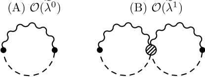
Figure 3: Diagrams contributing to $A^{c}(k,\omega)$ at (A) zeroth order and (B) first order in Eq. (13). The wavy (dashed) lines are the spinon (holon) propagators. The shaded vertex corresponds to $\widetilde{\lambda}$.

Turning to the calculation of the spectral function in the cartoon holon-metal phase described above, we find good comparison with recent temperature dependent photo-emission experiments in the normal “pseudo-gap” state of the cuprates mohit . In the cartoon state the propagators for the $z$ and $f$ field are, $G^{z}_{k,i\nu_{m}}\equiv-\langle zz^{\dagger}\rangle=-\frac{1}{\nu_{m}^{2}+E^{2}_{k}}$ and $G^{f}_{k,i\omega_{n}}\equiv-\langle ff^{\dagger}\rangle=\frac{1}{i\omega_{n}-\epsilon_{k}}$, where $E_{k}$ is the spinon dispersion and $\epsilon_{k}$ is the kinetic energy of the holons.

Neglecting fluctuations of the gauge field and setting $\widetilde{\lambda}=0$, Eq. (38) becomes after Fourier-transformation,

$$G^{c}_{k,i\omega_{n}}=2\sum_{P}\int\frac{d^{2}q}{(2\pi)^{2}}T\sum_{m}G^{z}_{q,i\nu_{m}}G^{f}_{q-k+K_{P},i\nu_{m}-i\omega_{n}}.$$ (40)

The spectral function of the electron is thus a convolution of the spectral functions of its composite “holon” and “spinon” particles, diagrammatically this may be simply represented as Fig. 3(A).

We can now easily complete the Matsubara sums and analytically continue $i\omega_{n}\rightarrow\omega+i\eta$, to obtain the expression for the spectral density $A=-2\Im[G^{R}]$. Note that the spectral functions do not satisfy the usual sum rule $\int\frac{d\omega}{2\pi}A(\omega)=1$ for fermions. This is because we are working the in projective subspace of the $t$-$J$ model.

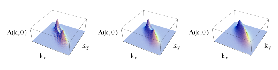
Figure 4: The change in the spectral response as the parameter $\eta$ (spectral broadening) is increased. In units of the spinon gap $T=0.5$. From left to right $\eta=0.2,0.4,0.8$. In the limit of perfect resolution the response consists of ellipses centered around the $\vec{K}_{p}$. The spectral peaks are due to the higher density of states perpendicular to the zone diagonals due to the larger holon mass in this direction. The rest of the results shown in this paper have $\eta=0.8$ to model the experimental resolution.

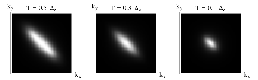
Figure 5: Evolution of $A^{c}_{\rm HM}(k,0)$ as a function of $T$ in the first quadrant of the square lattice BZ, calculated with Fig. 3A. These results bear close resemblance to the shrinking “Fermi Arcs” seen in photo-emission experiments on the underdoped cuprates mohit . The numerical evaluation of Eq. (41) was made with $m_{1\overline{x}}/m_{1\overline{y}}=0.05$ to model the anisotropic holon dispersion. These results are in the regime where the spectral resolution $\eta>T$, as in current experiments mohit . Note that this figure has $\widetilde{\lambda}=0$ and the “Fermi arcs” shrinks to $(\frac{\pi}{2},\frac{\pi}{2})$ at $T=0$.

Let us consider $\omega=0$ in the “holon-metal” phase, then Eq. (40) becomes,

$$A_{\rm HM}^{c}(k,0)=2\pi\frac{1}{V}\sum_{p,v}\frac{\delta(\epsilon-E)}{E}[n_{B}(E)+n_{F}(\epsilon)],$$ (41)

where we have used $\epsilon=\epsilon_{p-k+K_{P}}$ and $E=E_{p}$ for shorthand. Note that at $T=0$ this evaluates to zero and thus these contributions correspond to propagation of physical electrons in the presence of thermally excited spinons and holons. Using $\epsilon_{k}=\frac{k^{2}_{\overline{x}}}{2m_{v\overline{x}}}+\frac{k_{\overline{y}}^{2}}{2m_{v\overline{y}}}$ (for simplicity we set the chemical potential of the holons $\mu=0$) and $E_{k}=\sqrt{\Delta_{z}^{2}+c^{2}k^{2}}$, we can compute the zero energy spectral weight in $k$-space. We expect that $A(k,0)$ should have weight only for those momenta, $k$ at which a relative shift by $k$ of the spinon dispersion with respect to the holon dispersion causes the bottom of the gapped spinon dispersion to have the same energy as the holon. We thus expect spectral weights on ellipses centered around the $K_{p}$ points. We note however that current experiments are carried out in the regime where the spectral resolution (16-20meV) is larger than $T$ (110-200 K) mohit . For this reason, the ellipses predicted by our theory can not be resolved, as illustrated in Fig. 4. To make explicit contact with the experiments, we shall henceforth work in the regime where $\eta>T$ ($\eta$ is the imaginary part used in the analytic continuation).

The results are displayed in Fig. 5 as a function of the temperature $T$, they have many features similar to the spectral function measured in recent photo-emission experiments mohit . At finite-$T$, there are four “Fermi arcs” which have lengths that shrink with lowering $T$. In the holon-metal theory this shrinkage is due to that fact that as $T$ is lowered there are fewer and fewer thermally excited spinons present that are required to have an electronic excitation. An important difference between the experiments and the results presented in Fig. 5 is that in the photo-emission experiments in the pseudo-gap phase, the point to which the “Fermi arcs” shrink is shifted away from the $\vec{K}_{p}$. We now show that this observation follows on including the effect of Eq. (13).

We have so far excluded the “Shraiman-Siggia” term that couples the holons and the spinons, Eq. (13), i.e., we have used $\widetilde{\lambda}=0$. The first order correction to the $A^{c}$ due to Eq. (13) is given by the diagram shown in Fig. 3(B).

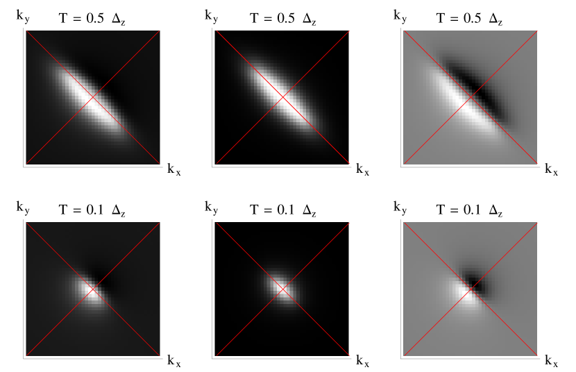
Figure 6: (color online) The first column shows the shift of the “nodal point” of Fermi arcs from the $\vec{K}_{p}$ on inclusion of the effect of Eq. (13) at first order in perturbation theory, Fig. 3B; the plot is of $A^{c}=A^{c(0)}+A^{c(1)}$. The next two show the individual contributions, $A^{c(0)}$ and $A^{c(1)}$. The second row is with the same physical parameters as the first set but at a lower $T=0.1\Delta_{z}$. All these data are in the regime where $\eta>T$. Lines joining $(0,0)$ to $(\pi,\pi)$ and $(0,\pi)$ to $(\pi,0)$ have been included for clarity.

We now focus on the momenta close to $K_{1}=(\frac{\pi}{2},\frac{\pi}{2})$ and hence drop the three other square lattice symmetry related terms. After Fourier transformation we obtain,

$$G^{c{(1)}}_{k+K_{1},i\omega_{n}} = \frac{2i\widetilde{\lambda}}{V^{2}}\left[2\sum_{p,q}i(k+p)_{x}f(p,q,k,i\omega_{n})\right]$$ (42)

where,

$$f(p,q,k,i\omega_{n}) = g(p,k,i\omega_{n})g(q,k,i\omega_{n}),$$

$$g(p,k,i\omega_{n}) = T\sum_{n_{1}}G^{f}_{p,i\omega_{n_{1}}}G^{z}_{k+p,i\omega_{n}+i\omega_{n_{1}}}$$ (43)

In order to calculate the spectral function we need to complete the Matsubara sums and then continue $i\omega_{n}\rightarrow\omega+i\eta$ and get the imaginary part of $f$. Note that because one can always put $p\rightarrow-p$ in the sums above the spectral function contribution changes sign when $k_{x}\rightarrow-k_{x}$, i.e. depending on the sign of $\widetilde{\lambda}$, it shifts the spectral weight in $A^{c}(k,0)$ towards(away) from the $\Gamma$-point along the zone diagonal.

For $\omega=0$, we obtain for the function $g(p,k,\omega=0)$,

$$\Re[g] = \frac{1}{2E}\left[\frac{n_{B}(E)-n_{F}(\epsilon)+1}{E+\epsilon}-\frac{n_{B}(E)+n_{F}(\epsilon)}{E-\epsilon}\right]$$

$$\Im[g] = -\frac{\pi}{2E}[n_{B}(E)+n_{F}(\epsilon)]~{}~{}\delta(E-\epsilon).$$ (44)

where we have uses the short-hand, $E=E_{k+p}$ and $\epsilon=\epsilon_{p}$.

We now evaluate the sums in Eq. (42) numerically. Results are presented in Fig. 6. Inclusion of the $\widetilde{\lambda}$ term does not change the general features of the shrinking “Fermi arcs” observed in Fig. 5, instead it shifts the nodal point away from the $\vec{K}_{p}$, just as is seen in the experiments. It should be noted that the holons still have their dispersion minima at the $\vec{K}_{p}$, only the physical electrons have their spectral weight shifted away from $\vec{K}_{p}$ because of $\widetilde{\lambda}$. This should be contrasted with the long-range ordered Néel phase where even Eq. (13) cannot change the pinning of the center of the spectral weight away from the $\vec{K}_{p}$ (as observed in experimentskim ).

VI Conclusions

The starting point of this paper was the deconfined quantum critical point between the Néel and VBS ground states of a $S=1/2$ square lattice antiferromagnet. We added a small density of holes to both states and found distinct Fermi liquid states. Their difference was characterized in Eq. (1), and ultimately had its origin in the following results: (i) the dispersion of a single hole in a Néel state can have the minimum of its dispersion pinned at the symmetrical points $\vec{K}_{p}$ (Fig 2) over a finite range of parameters; (ii) the minimum of the dispersion of a single hole in the VBS state is generically shifted away from the $\vec{K}_{p}$, as established in Eq. (34); the binding of the holon and spinon into a charge $e$ $S=1/2$ quasiparticle in the VBS phase was crucial in obtaining this shift. We also argued that at finite hole doping, $\delta$, these Fermi liquid states were likely not connected by a direct quantum phase transition, but that the insulating deconfined quantum critical point opened up into a non-Fermi-liquid holon metal phase.

We also discussed the finite temperature, “quantum critical”, holon metal phase obtained above the low-temperature ordered phases. The spectra shown in Section V.1 were found to be consistent with key characteristics of recent observations of “Fermi-arc” spectra in the pseudogap phase of the cuprates. In particular, we showed that the peak in the spectral weight was shifted away from the symmetrical $\vec{K}_{p}$ position. This shift was linked to the same term in the Lagrangian that caused the shift of the dispersion minimum in the VBS state, a term originally introduced by Shraiman and Siggia ss .

Finally, we note that our boundary CFT in Section V has features that are reminiscent of self-consistent impurity models qsi1 of ‘local’ quantum phase transitions in Kondo lattice systems. However, the details are different, and can only be addressed in a quantum field-theoretic framework which we have described. This work therefore also serves to place studies of quantum transitions in the ‘dynamical mean field theory’ approach qsi1 ; gabi in the field-theoretic context.

Appendix A Single hole in the U(1) spin liquid

In this appendix, we calculate the dispersion of the holons due to absorption and emission of the spinons. We will work within the framework of the $t-J$ model Eq. (2), using the formalism of Refs. klr, ; suyu, .

First consider the second term in Eq. (2), using a Schwinger-boson mean-field theory aa , we arrive at Eq. (6). After Fourier transformation, this Hamiltonian can be diagonalized into the form

$$H_{J}=\sum_{k\sigma}\epsilon_{k}(\alpha^{\dagger}_{k\sigma}\alpha_{k\sigma}+\beta^{\dagger}_{k\sigma}\beta_{k\sigma})$$ (45)

by introducing two new particles,

$$\alpha_{k\sigma} = u_{k}b_{k\sigma}+v_{k}\overline{b}^{\dagger}_{-k\sigma}$$

$$\beta_{k\sigma} = u_{k}\overline{b}_{k\sigma}+v_{k}b^{\dagger}_{-k\sigma}\,,$$ (46)

where

$$\gamma_{k}=\sum_{\delta}e^{ik\cdot\delta}=2\left[\cos\left(\frac{k^{\prime}_{x}+k^{\prime}_{y}}{2}a^{\prime}\right)+\cos\left(\frac{k^{\prime}_{x}-k^{\prime}_{y}}{2}a^{\prime}\right)\right]$$ (47)

where $k^{\prime}_{x(y)}\in[-\frac{\pi}{a^{\prime}},\frac{\pi}{a^{\prime}}]$ (i.e. BZ^′), where $a^{\prime}=\sqrt{2}a$. $u(v)_{k}$ are real and $u(v)_{k}=u(v)_{-k}$. A comparison of terms gives, $u_{k}=\cosh\theta_{k}$ and $v_{k}=\sinh\theta_{k}$, where $\tanh 2\theta_{k}=-Q\gamma_{k}/\lambda$. The dispersion of the $\alpha,\beta$ quasiparticles is $\epsilon_{k}=(\lambda^{2}-(Q\gamma_{k})^{2})^{1/2}$. Using these we can calculate all the propagators of interest,

$$-\langle b_{k\sigma}b^{\dagger}_{k\sigma}\rangle = -\frac{i\nu_{n}+\lambda}{\nu_{n}^{2}+\epsilon_{k}^{2}}\equiv\mathcal{G}(k,i\nu_{n})$$ (48)

$$-\langle b_{k\sigma}\overline{b}_{-k\sigma}\rangle = -\frac{Q\gamma_{k}}{\nu_{n}^{2}+\epsilon_{k}^{2}}\equiv\mathcal{F}(k,i\nu_{n})$$ (49)

We now define $\alpha=Q/\lambda$ and use this parameter instead of $Q$. Then, e.g., the dispersion becomes $\epsilon_{k}=\lambda(1-(\alpha\gamma_{k})^{2})^{1/2}$, where $0<\alpha<0.25$.

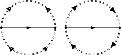
Figure 7: The two diagrams contributing to the holon self-energy in Eq. (51). The solid lines are the holon propogators and the double-dashed lines are the spinons.

The hopping term in the $t-J$ model in terms of Schwinger bosons after Fourier transformation gives,

$$H_{t}=t\sum_{k,q_{1},q_{2}}\gamma_{k}\varepsilon_{\sigma\sigma^{\prime}}(f_{+,q_{1}}b^{\dagger}_{k+q_{1}\sigma}\overline{b}_{k+q_{2}\sigma^{\prime}}f^{\dagger}_{-,q_{2}}+f_{-,q_{1}}\overline{b}^{\dagger}_{k+q_{1}\sigma^{\prime}}b_{k+q_{2}\sigma}f^{\dagger}_{+,q_{2}})$$ (50)

Working to second order in the hopping, we now calculate the self-energy of the $f_{\pm}$ particles due to the $H_{t}$. There are two diagrams at order $t^{2}$ (shown in Fig. 7) that need to be summed up, they evaluate to,

$$\Sigma^{A}_{1}(k,i\omega_{n}) = [2]t^{2}\frac{1}{\beta^{2}}\sum\gamma_{q-p}^{2}\mathcal{G}(i\nu_{m},q)\mathcal{G}(i\omega_{n}-i\omega_{l}+i\nu_{m},k+q-p)\mathcal{G}^{B}_{f}(i\omega_{l},p)$$ (51)

$$\Sigma^{A}_{2}(k,i\omega_{n}) = [-2]t^{2}\frac{1}{\beta^{2}}\sum\gamma_{q-p}\gamma_{q+k}\mathcal{F}(i\nu_{m},q)\mathcal{F}(i\omega_{n}-i\omega_{l}+i\nu_{m},k+q-p)\mathcal{G}^{B}_{f}(i\omega_{l},p)$$

The factors in $[...]$ appear from the spin sums. The sum of the above diagrams becomes (we assume here that $A(p,\omega<0)=0$),

$$\Sigma^{A}(i\omega_{n},k)=\sum_{q,p}[t^{2}(\gamma_{q-p}u_{k+q-p}v_{q}-\gamma_{q+k}u_{q}v_{k+q-p})^{2}]\mathcal{G}^{B}_{f}(i\omega_{n}-\epsilon_{q}-\epsilon_{k+q-p},k)$$ (52)

A full self-consistent solution of the above equation corresponds to summing all diagrams that have non-crossing boson lines. The dispersion of the f-particles is obtained by looking for the poles of the interacting Greens’ function, i.e. $\omega_{k}=\Re[\Sigma(\omega_{k},k)]$. We shall not undertake the fully self-consistent calculation here, instead we simply use the self energy to second-order in $t$ which gives.

$$\omega_{k}=\sum_{q,p}F_{t^{2}}(k,p,q)\frac{1}{-\epsilon_{k+q-p}-\epsilon_{q}},$$ (53)

where $F_{t^{2}}(k,p,q)=t^{2}(\gamma_{q-p}u_{k+q-p}v_{q}-\gamma_{q+k}u_{q}v_{k+q-p})^{2}$. This result is plotted in Fig. 8. As discussed in the text, the holon disperion has minima at the $(\pm\pi/2,\pm\pi/2)$. The band masses at the minima are highly anisotropic with the holon dispersion much lighter along the zone diagonal than perpendicular to it.

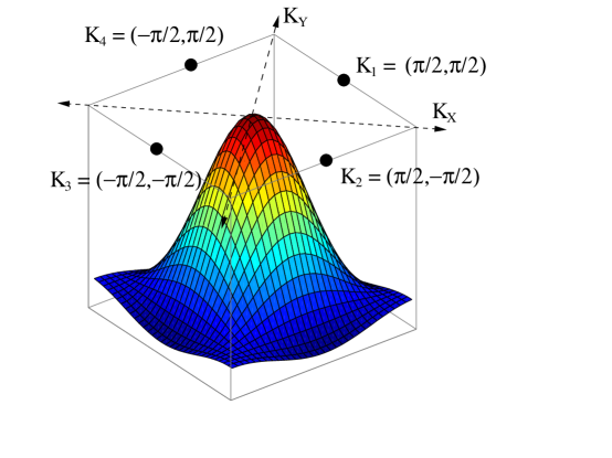
Figure 8: (color online) The dispersion $\omega_{k}t^{2}/\lambda$ obtained from Eq. (53). The points $K_{p}$ where the holon dispersion have their minima are marked for clarity. We have used $\alpha=0.24$ here, note however that these results are generic.

Appendix B Critical properties of the $\mathbb{CP}^{N-1}$ model

As argued elsewhere, and reviewed in Section I, the critical theory of the Néel-VBS transition on the square lattice is described by the $\mathbb{CP}^{N-1}$ model. Here we will review the $1/N$ expansion of this theory, obtain an effective field theory suitable for bound state problems, and compute a scaling dimension in the boundary CFT associated with a charged impurity.

We are interested in the properties of the field theory

$$Z = \int\mathcal{D}z_{\alpha}\mathcal{D}\lambda\mathcal{D}A_{\mu}\exp\left(-\mathcal{S}\right)$$

$$\mathcal{S} = \int d^{2}rd\tau\left[\frac{1}{g}\left\{|(\partial_{\mu}-iA_{\mu})z_{\alpha}|^{2}+i\lambda(|z_{\alpha}|^{2}-N)\right\}\right]$$ (54)

Here the index $\alpha=1\ldots N$, and $\tau$ is imaginary time. The theory has a conformally invariant critical point at a $g=g_{c}$, and we want to describe the spectrum for $g>g_{c}$.

First, let us review the properties at $N=\infty$. The quantum critical point is at $g=g_{c}$, where

$$\frac{1}{g_{c}}=\int_{0}^{\Lambda}\frac{d^{3}p}{8\pi^{3}}\frac{1}{p^{2}}$$ (55)

Here, $\Lambda$ is an ultraviolet cutoff, and we will only be interested in phenomena at scales much smaller than $\Lambda$.

For $g>g_{c}$, we have a large $N$ solution for the spin-gap U(1) spin liquid with $\langle z_{\alpha}\rangle=0$, $i\lambda=\Delta_{0}^{2}$, where

$$\int_{0}^{\infty}\frac{d^{3}p}{8\pi^{3}}\left(\frac{1}{p^{2}}-\frac{1}{p^{2}+\Delta_{0}^{2}}\right)=\frac{1}{g_{c}}-\frac{1}{g}$$ (56)

Here $\Delta_{0}$ is a measure of the spin gap at $N=\infty$; we will discuss the renormalization of this to the energy scale $\Delta$ in the following subsection.

For $g<g_{c}$, we have the Néel phase, which breaks the SU($N$) rotation symmetry with $\langle z_{\alpha}\rangle=m_{0}\sqrt{N}\delta_{\alpha,1}$ and $i\lambda=0$. The value of $m_{0}$ is given by

$$m_{0}^{2}=\frac{1}{g}-\frac{1}{g_{c}}$$ (57)

The properties of this phase are easy to understand by spin-wave theory (“chiral perturbation theory”), and we won’t consider it further.

We now consider the structure of fluctuations for $g\geq g_{c}$. The $1/N$ expansion can be easily generated by a Feynman graph expansion of the theory

$$Z = \int\mathcal{D}z_{\alpha}\mathcal{D}\lambda\mathcal{D}A_{\mu}\exp\left(-\mathcal{S}\right)$$ (58)

$$\mathcal{S} = \int d^{2}rd\tau\left[\left\{|(\partial_{\mu}-iA_{\mu})z_{\alpha}|^{2}+\Delta_{0}^{2}|z_{\alpha}|^{2}+i\lambda|z_{\alpha}|^{2}\right\}\right]$$

$$~{}~{}~{}~{}~{}~{}~{}~{}~{}~{}~{}~{}+\int\frac{d^{3}p}{8\pi^{3}}\left[\frac{N}{2}\Pi(p)|\lambda(p)|^{2}+\frac{N}{2}K(p)A_{\mu}(-p)\left(\delta_{\mu\nu}-\frac{p_{\mu}p_{\nu}}{p^{2}}\right)A_{\nu}(p)\right].$$

Here we have rescaled $z_{\alpha}$ by $\sqrt{g}$, and there is no further dependence upon $g$. The kernels $\Pi(p)$ and $K(p)$ represent one-loop $z_{\alpha}$ contributions. We avoid double counting in the Feynman graph expansion simply by avoiding any further bubble self-energy contributions to the $\lambda$ and $A_{\mu}$ propagators. The explicit values of the kernels are

$$\Pi(p) = \int\frac{d^{3}q}{8\pi^{3}}\frac{1}{(q^{2}+\Delta_{0}^{2})((p+q)^{2}+\Delta_{0}^{2})}$$ (61)

$$= \frac{1}{4\pi p}\cot^{-1}\left(\frac{2\Delta_{0}}{p}\right)$$

$$= \left\{\begin{array}[]{ccc}1/(8\pi\Delta_{0})&{}{}\hfil&p\ll\Delta_{0}\\ 1/(8p)&{}{}{}\hfil&p\gg\Delta_{0}\end{array}\right.$$

and

$$K(p) = -2\int\frac{d^{3}q}{8\pi^{3}}\frac{q^{2}-(p\cdot q)^{2}/p^{2}}{((q+p/2)^{2}+\Delta_{0}^{2})((q-p/2)^{2}+\Delta_{0}^{2})}+2\int\frac{d^{3}q}{8\pi^{3}}\frac{1}{q^{2}+\Delta_{0}^{2}}$$ (64)

$$= \int_{0}^{1}\frac{dx}{2\pi}\left[\sqrt{p^{2}x(1-x)+\Delta_{0}^{2}}-\Delta_{0}\right]$$

$$= \frac{p^{2}+4\Delta_{0}^{2}}{8\pi p}\cot^{-1}\left(\frac{2\Delta_{0}}{p}\right)-\frac{\Delta_{0}}{4\pi}$$

$$= \left\{\begin{array}[]{ccc}p^{2}/(24\pi\Delta_{0})&{}{}\hfil&p\ll\Delta_{0}\\ p/16&{}{}{}\hfil&p\gg\Delta_{0}\end{array}\right.,$$

where we have used the Feynman parameter method to evaluate the integrals.

The following subsection will formulate an approach suitable for bound state problems, and examine the response to an impurity.

B.1 Non-relativistic effective field theory

We are interested here primarily in the physics at scales $p\lesssim\Delta_{0}$. As in ordinary quantum electrodynamics, this regime is conveniently expressed in terms of a non-relativistic effective field theory. We will see that the low-velocity expansion associated with the effective field theory is justified because the typical velocity in a bound state scales as $1/\sqrt{N}$.

We first need to express the relativistic theory in (58) in terms of the non-relativistic particle and anti-particle eigenstates. To this end, we decouple the kinetic term for the $z_{\alpha}$ by a Hubbard-Stratanovich field $\Pi_{\alpha}$:

$$|(\partial_{\tau}-iA_{\tau})z_{\alpha}|^{2}\rightarrow|\Pi_{\alpha}|^{2}+i\Pi_{\alpha}^{\ast}(\partial_{\tau}-iA_{\tau})z_{\alpha}+\mbox{c.c.}$$ (65)

Then we parameterize

$$z_{\alpha} = \frac{1}{\sqrt{2\Delta_{0}}}\left(p_{\alpha}+h_{\alpha}^{\dagger}\right)$$

$$\Pi_{\alpha} = \frac{1}{\sqrt{2\Delta_{0}}}\left(p_{\alpha}-h_{\alpha}^{\dagger}\right)\,$$ (66)

where $p_{\alpha}$ and $h^{\alpha}$ will be the spinon and anti-spinon excitations. For the SU(2) case, with $N=2$, we will make the replacement $h^{\alpha}\rightarrow\varepsilon^{\alpha\beta}h_{\beta}$, so that both the spinons and anti-spinons transform under the same representation of SU(2).

We now insert (66) in the effective action (58), and expand in powers of spatial gradients. The structure of this expansion determines the form of the effective field theory. With some additional approximations which will shortly be justified, we postulate, up to order $1/N$, the following non-relativistic effective field theory

$$Z_{NR} = \int\mathcal{D}p_{\alpha}\mathcal{D}h_{\alpha}\mathcal{D}A_{\tau}\exp\left(-\mathcal{S}_{NR}\right)$$

$$\mathcal{S}_{NR} = \int d^{2}rd\tau\left[\frac{N}{48\pi\Delta}(\vec{\nabla}A_{\tau})^{2}+p^{\alpha\dagger}\left(\frac{\partial}{\partial\tau}-iA_{\tau}+\Delta\left(1+\frac{\zeta_{1}}{N}\right)-\frac{1}{2\Delta}\vec{\nabla}^{2}\right)p_{\alpha}\right.$$ (67)

$$~{}~{}~{}~{}~{}~{}~{}~{}~{}~{}~{}~{}~{}~{}+\left.h^{\dagger}_{\alpha}\left(\frac{\partial}{\partial\tau}+iA_{\tau}+\Delta\left(1+\frac{\zeta_{1}}{N}\right)-\frac{1}{2\Delta}\vec{\nabla}^{2}\right)h^{\alpha}\right]$$

Here we have defined the renormalized energy scale $\Delta$ so that the co-efficient of the electrostatic term $(\vec{\nabla}A_{\tau})^{2}$ term is $N/(48\pi\Delta)$. At $N=\infty$, we have $\Delta=\Delta_{0}$; there will be corrections at order $1/N$, which can be computed from (58), which will depend upon the cutoff $\Lambda$, and which ensure that $\Delta\sim(g-g_{c})^{\nu}$, with irkhin $\nu=1-48/(\pi^{2}N)$. The numerical constant $\zeta_{1}$ is a universal number to be determined by a matching computation to the fully relativistic theory (58); we will not carry out such a computation here.

The dominant interaction is the ‘Coulomb’ interaction between the $p_{\alpha}$ and the $h^{\alpha}$, mediated by the electrostatic potential $A_{\tau}$. This leads to a potential energy between opposite unit charges of the form

$$V(r) = \frac{24\pi\Delta}{N}\int^{~{}\sim\Delta}\frac{d^{2}k}{4\pi^{2}}\frac{(1-e^{i\vec{k}\cdot\vec{r}})}{k^{2}}$$ (68)

$$= \frac{12\Delta}{N}\left[\ln\left(r\Delta\right)+\zeta_{2}\right]\,.$$

Here $\zeta_{2}$ appears to be a second unknown constant, but we have the freedom to set $\zeta_{2}=0$ without modifying any observable property. This is because $Z_{NR}$ applies only to spinon/anti-spinon configurations which have net charge zero, and for these $\zeta_{2}$ can be absorbed into a redefinition of $\zeta_{1}$.

From this potential we see that the spinon and anti-spinon form a bound state with a spatial extent $\sim\sqrt{N}/\Delta$. This means that the velocity expansion holds in powers of $1/\sqrt{N}$. One can also see from this that the coupling to the spatial components of the gauge field, $\vec{A}$, lead to corrections which are higher order in $1/N$ from the terms included. Short-range interaction terms (induced from $\lambda$ fluctuations) like $|p_{\alpha}|^{2}|h^{\alpha}|^{2}$ are also easily seen in perturbation theory to be higher order: they induce corrections which depend upon the value of the bound state function at the origin $\sim 1/\sqrt{N}$. These arguments justify our dropping $\lambda$ and $\vec{A}$ fluctuations in $Z_{NR}$.

B.2 Boundary exponent of an impurity

As motivated in Section V, we consider here the problem of a static charged impurity coupled to the 2+1 dimensional critical point of $\mathbb{CP}^{N-1}$ model. For this we modify the theory in Eq. (54) to

$$\widetilde{Z} = \int\mathcal{D}z_{\alpha}\mathcal{D}f\mathcal{D}\lambda\mathcal{D}A_{\mu}\exp\left(-\widetilde{\mathcal{S}}\right)$$

$$\widetilde{\mathcal{S}} = \int d^{2}rd\tau\mathcal{L}_{z}+\int d\tau f^{\dagger}\left(\frac{\partial}{\partial\tau}+\varepsilon_{0}-iA_{\tau}(r=0,\tau)\right)f,$$ (69)

$$\mathcal{L}_{z} = |(\partial_{\mu}-ie_{0}A_{\mu})z_{\alpha}|^{2}+s|z_{\alpha}|^{2}+\frac{u_{0}}{2}\left(|z_{\alpha}|^{2}\right)^{2}$$

$$~{}~{}~{}~{}~{}~{}~{}~{}~{}+\frac{1}{2}\left(\epsilon_{\mu\nu\lambda}\partial_{\nu}A_{\lambda}\right)^{2},$$

Note that the Grassman field $f$ depends only upon $\tau$, while the bosonic fields vary over both $r$ and $\tau$. For completeness, we add “bare” terms corresponding to the spinon interaction and the gauge field kinetic energy, and we will see that the critical exponents are independent of these terms. We will now compute the scaling dimension $\eta_{h}/2$ of the composite operator $h(\tau)=z_{\alpha}(r=0,\tau)f^{\dagger}(\tau)$.

At the critical point $s=s_{c}$, the bare boson propagator is $G_{0}(k)=1/k^{2}$. The dressed photon propagator can be obtained by summing over $z$-bubbles and has the form

$$D_{\mu\nu}(p)=(p^{2}+\gamma p)^{-1}\Big{(}\delta_{\mu\nu}-\zeta\frac{p_{\mu}p_{\nu}}{p^{2}}\Big{)},$$ (70)

where $\zeta$ is the arbitrary “gauge parameter” and

$$\gamma=Ne_{0}^{2}/16.$$

In a similar way, one can obtain the dressed $z$-field interaction vertex

$$V(k)=\frac{u_{0}}{1+2u_{0}N\Pi(k)},$$

where $\Pi(k)=1/(8k)$ is the bosonic bubble. The large-$N$ expansion is thus the expansion in dressed photon lines and dressed $z$-vertices.

The anomalous dimensions $\eta_{z}$ and $\eta_{f}$ of the fields $z$ and $f$ can be read off as the coefficients in the contributions of the type $-\eta_{z}p^{2}\ln(p)$ and $i\eta_{f}\omega\ln(\omega)$ to the self-energies $\Sigma_{z}(p)$ and $\Sigma_{f}(\omega)$ which enter the corresponding dressed propagators $G^{-1}(p)=p^{2}+\Sigma_{z}(p)$ and $G_{f}^{-1}(\omega)=-i\omega+\Sigma_{f}(\omega)$ (here $\omega$ is counted from the reference energy $\varepsilon_{0}$). To the order of $1/N$, the self-energies are given by

$$\Sigma_{z}(p) = \int\frac{d^{3}k}{(2\pi)^{3}}G_{0}(p-k)\Big{\{}2V(k)$$ (71)

$$- e_{0}^{2}(2p_{\mu}-k_{\mu})(2p_{\nu}-k_{\nu})D_{\mu\nu}(k)\Big{\}},$$

$$\Sigma_{f}(\omega) = e_{0}^{2}\int\frac{d^{3}k}{(2\pi)^{3}}\frac{1}{-i(\omega-\Omega)}D_{00}\big{(}k=(q,\Omega)\big{)}$$ (72)

and after tedious but straightforward calculation one obtains

$$\eta_{z}=\frac{4}{3\pi^{2}N}-\frac{4e_{0}^{2}}{3\pi^{2}\gamma}-(1-\zeta)\frac{e_{0}^{2}}{2\pi^{2}\gamma},$$ (73)

$$\eta_{f}=-(1+\zeta)\frac{e_{0}^{2}}{2\pi^{2}\gamma},$$ (74)

One should realize that, taken separately, $\eta_{z}$ and $\eta_{f}$ are both gauge-dependent and do not have any direct physical sense. It turns out that there is no contribution to $\eta_{h}$ from the vertex diagram describing an exchange of a photon between the $z$ and $f$ particles, so to the $1/N$ order, the scaling dimension $\eta_{h}/2$ of $h$ is given by $1/2+\eta_{z}+\eta_{f}$, which in turn yields the (gauge-independent) expression (37) for the boundary exponent $\eta_{h}$.

References

- (1) S. A. Trugman, Phys. Rev. B 37, 1597 (1988).
- (2) C. L. Kane, P. A. Lee, and N. Read, Phys. Rev. B 39, 6880 (1989).
- (3) S. Sachdev, Phys. Rev. B 39, 12232 (1989).
- (4) V. Elser, D. A. Huse, B. I. Shraiman, and E. D. Siggia, Phys. Rev. B 41, 6715 (1990).
- (5) G. Martínez and P. Horsch, Phys. Rev. B 44, 317 (1991).
- (6) D. Poilblanc, H. J. Schulz, and T. Ziman, Phys. Rev. B 47, 3268 (1993).
- (7) G. F. Reiter, Phys. Rev. B 49, 1536 (1994).
- (8) A. S. Mishchenko, N. V. Prokof’ev, and B. V. Svistunov, Phys. Rev. B 64, 033101 (2001).
- (9) B. I. Shraiman and E. D. Siggia, Phys. Rev. Lett. 61, 467 (1988).
- (10) F. Kämpfer, M. Moser, and U.-J. Wiese, Nucl. Phys. B 729, 317 (2005); C. Brügger, F. Kämpfer, M. Moser, M. Pepe, and U.-J. Wiese, Phys. Rev. B 74, 224432 (2006).
- (11) T. Senthil, A. Vishwanath, L. Balents, S. Sachdev, and M. P. A. Fisher, Science 303, 1490 (2004); T. Senthil, L. Balents, S. Sachdev, A. Vishwanath, and M. P. A. Fisher, Phys. Rev. B 70, 144407 (2004).
- (12) A. Kuklov, N. Prokof’ev, B. Svistunov, and M. Troyer, Annals of Physics 321, 1602 (2006) have studied a particular lattice realization of the ‘easy-plane’ limit of the field theory proposed in Ref. senthil1, , and found a first-order transition. This does not rule out a second-order transition for other lattice realizations. A second-order, deconfined, transition has been theoertically established for sufficiently large, but finite. There is also strong numerical evidence for a continuous transition for the physically interesting case with and full SU(2) symmetryanders ; kamal ; mv .
- (13) A. W. Sandvik, cond-mat/0611343.
- (14) M. Kamal and G. Murthy, Phys. Rev. Lett. 71, 1911 (1993).
- (15) O. I. Motrunich and A. Vishwanath, Phys. Rev. B 70, 075104 (2004).
- (16) M. Levin and T. Senthil, Phys. Rev. B 70, 220403(R) (2004).
- (17) A. Kanigel, M. R. Norman, M. Randeria, U. Chatterjee, S. Suoma, A. Kaminski, H. M. Fretwell, S. Rosenkranz, M. Shi, T. Sato, T. Takahashi, Z. Z. Li, H. Raffy, K. Kadowaki, D. Hinks, L. Ozyuzer, and J. C. Campuzano, Nature Physics 2, 447 (2006).
- (18) P. Coleman and A. J. Schofield, Nature 433, 226 (2005).
- (19) Q. Si, cond-mat/0601001.
- (20) T. Senthil, S. Sachdev, and M. Vojta, Physica B 359-361, 9 (2005); T. Senthil, Annals of Physics, 321, 1669 (2006).
- (21) H. Shishido, R. Settai, H. Harima, and Y. Onuki, J. Phys. Soc. Jpn. 74, 1103 (2005).
- (22) X.-G. Wen, Phys. Rev. B 39, 7223 (1989).
- (23) R. Shankar, Phys. Rev. Lett. 63, 203 (1989).
- (24) P. A. Lee, Phys. Rev. Lett. 63, 680 (1989).
- (25) S. K. Sarker, cond-mat/0701288.
- (26) M. Hermele, T. Senthil, M. P. A. Fisher, P. A. Lee, N. Nagaosa, and X.-G. Wen, Phys. Rev. B 70, 214437 (2004).
- (27) A similar perspective was taken for a Landau-Ginzburg-Wilson transition in an antiferromagnet in M. Vojta, C. Buragohain, and S. Sachdev, Phys. Rev. B 61, 15152 (2000), and for the doped ‘staggered flux’ algebraic spin liquid in T. Senthil and P. A. Lee, Phys. Rev. B 71, 174515 (2005).
- (28) A. Paramekanti and E. Zhao, cond-mat/0611762.
- (29) A. Abanov, A. V. Chubukov, and J. Schmalian, Adv. Phys. 52, 119 (2003).
- (30) N. Read and S. Sachdev, Phys. Rev. Lett. 62, 1694 (1989); Phys. Rev. B 42, 4568 (1990).
- (31) D. P. Arovas and A. Auerbach, Phys. Rev. B 38, 316 (1988).
- (32) X.-G. Wen, Phys. Rev. B 65, 165113 (2002).
- (33) L. Balents and S. Sachdev, cond-mat/0612220.
- (34) F. D. M. Haldane, Phys. Rev. Lett. 61, 1029 (1988).
- (35) Y. M. Li, D. N. Sheng, Z. B. Su, and L. Yu, Phys. Rev. B 45, 5428 (1992).
- (36) D. Sénéchal, P.-L. Lavertu, M.-A. Marois, and A.-M. S. Tremblay, Phys. Rev. Lett. 94, 156404 (2005).
- (37) A. Kolezhuk, S. Sachdev, R. R. Biswas, and P. Chen, Phys. Rev. B 74, 165114 (2006).
- (38) G. Murthy and S. Sachdev, Nucl. Phys. B 344, 557 (1990).
- (39) T. Senthil, S. Sachdev, and M. Vojta, Phys. Rev. Lett. 90, 216403 (2003); T. Senthil, M. Vojta, and S. Sachdev, Phys. Rev. B 69, 035111 (2004).
- (40) S. Sachdev, M. Troyer, and M. Vojta, Phys. Rev. Lett. 86, 2617 (2001).
- (41) W. Rantner and X.-G. Wen, cond-mat/0105540.
- (42) J. Ye, Phys. Rev. B 67, 115104 (2003).
- (43) H. Kleinert and A. M. J. Schakel, Phys. Rev. Lett. 90, 097001 (2003).
- (44) Z. Y. Weng, V. N. Muthukumar, D. N. Sheng, and C. S. Ting, Phys. Rev. B 63, 075102 (2001).
- (45) C. Kim, P. J. White, Z.-X. Shen, T. Tohyama, Y. Shibata, S. Maekawa, B. O. Wells, Y. J. Kim, R. J. Birgeneau, and M. A. Kastner, Phys. Rev. Lett. 80, 4245 (1998).
- (46) Q. Si, S. Rabello, K. Ingersent, and J. L. Smith, Nature 413, 804 (2001).
- (47) A. Georges, G. Kotliar, W. Krauth, and M. Rozenberg, Rev. Mod. Phys. 68, 13 (1996).
- (48) V. Yu. Irkhin, A. A. Katanin, and M. I. Katsnelson, Phys. Rev. B 54, 11953 (1996).