Predictions of Dynamic Behavior Under Pressure for Two Scenarios to Explain Water Anomalies

Abstract

Using Monte Carlo simulations and mean field calculations for a cell model of water we find a dynamic crossover in the orientational correlation time $\tau$ from non-Arrhenius behavior at high temperatures to Arrhenius behavior at low temperatures. This dynamic crossover is independent of whether water at very low temperature is charaterized by a “liquid-liquid critical point” or by the “singularity free” scenario. We relate $\tau$ to fluctuations of hydrogen bond network and show that the crossover found for $\tau$ for both scenarios is a consequence of the sharp change in the average number of hydrogen bonds at the temperature of the specific heat maximum. We find that the effect of pressure on the dynamics is strikingly different in the two scenarios, offering a means to distinguish between them.

Two different scenarios are commonly used to interpret the anomalies of water angellreview ; pabloreview :

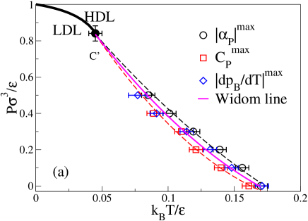
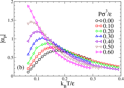
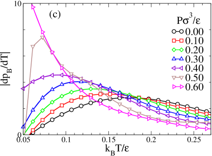
Figure 1: (color online) (a) The relevant part of the liquid phase diagram for the LLCP scenario. $C^{\prime}$ is the LDL-HDL critical point at the end of the first-order phase transition line (thick line) fs , $T_{W}(P)$ (thin line) is the Widom line, which we take to be the average between $T(|\alpha_{P}|^{\rm max})$ ($\bigcirc$) and $T(C_{P}^{\rm max})$ ($\Box$) from panel (b), and Fig. 2(a), respectively. Upper and lower dashed line are quadratic fits of $|\alpha_{P}|^{\rm max}$ and $C_{P}^{\rm max}$, respectively, merging at the $C^{\prime}$. $T(|\alpha_{P}|^{\rm max})$ and $T(C_{P}^{\rm max})$ overlap within the error bars. (b) $|\alpha_{P}|$ as a function of $T$ for different $P$. (c) $|dp_{\rm B}/dT|$, the temperature derivative of $p_{\rm B}$, as a function of $T$ for different $P$. In panel (a), $T(|dp_{\rm B}/dT|^{\rm max})$ ($\Diamond$) overlaps $T_{W}(P)$.

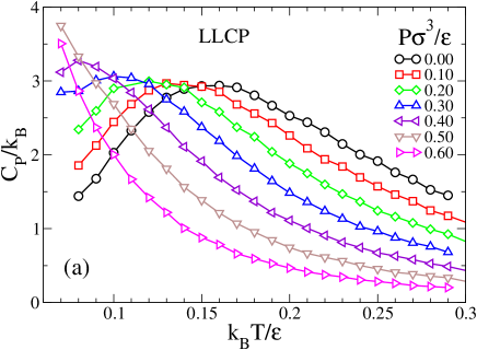
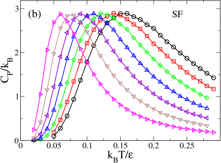
Figure 2: (color online) Temperature dependence of the specific heat $C_{P}$ for both the LLCP and the SF scenarios, for seven values of $P$. (a) For the LLCP scenario, $C_{P}$ has a maximum, the size of which increases with increasing pressure and diverges as $P\rightarrow P_{C^{\prime}}$. (b) For the SF scenario, $C_{P}$ also has a maximum, but its size does not increase with increasing pressure, consistent with the findings of the mean field calculations of Ref. sdss .

• The liquid-liquid critical point (LLCP) scenario hypothesizes that supercooled water has a liquid-liquid phase transition line that separates a low-density liquid (LDL) at low temperature $T$ and low pressure $P$ and a high-density liquid (HDL) at high $T$ and $P$ and terminates at a critical point $C^{\prime}$ Mishima1998nature . From $C^{\prime}$ emanates the Widom line $T_{W}(P)$, the line of maximum correlation length in the $(T,P)$ plane. Response functions, such as the isobaric heat capacity $C_{P}$, the coefficient of thermal expansion $\alpha_{P}$, and the isothermal compressibility $K_{T}$, have maxima along lines that converge toward $T_{W}(P)$ upon approaching $C^{\prime}$ [Figs. 1 and 2(a)].

• The singularity-free (SF) scenario hypothesizes the presence of a line of temperatures of maximum density $T_{\rm MD}(P)$ with negative slope in the $(T,P)$ plane. As a consequence, $K_{T}$ and $|\alpha_{P}|$ have maxima that increase upon increasing $P$, as shown using a cell model of water. The maxima in $C_{P}$ do not increase with $P$, suggesting that there is no singularity sdss [Fig. 2(b)].

Above the homogeneous nucleation line $T_{H}(P)$ where data are available, the two scenarios predict roughly the same equilibrium phase diagram. Here we show that dynamic measurements should reveal a striking difference between the two scenarios. Specifically, the low-$T$ dynamics depends on local structural changes, quantified by the variation of the number of hydrogen bonds, that are affected by pressure differently for each scenario. We find this result by studying—using Monte Carlo (MC) simulations and mean field calculations—a cell model which has the property that by tuning a parameter its predictions conform to those of either the LLCP or the SF scenario. This cell model is based on the experimental observations that on decreasing $P$ at constant $T$, or on decreasing $T$ at constant $P$, (i) water displays an increasing local tetrahedrality Darrigo81 , (ii) the volume per molecule increases at sufficiently low $P$ or $T$, and (iii) the O-O-O angular correlation increases Bosio83 .

The entire system is divided into cells $i\in[1,\ldots,N]$, each containing a molecule with volume $v\equiv V/N$, where $V\geq Nv_{\rm hc}$ is the total volume of the system, and $v_{\rm hc}$ is the hard-core volume of one molecule. The cell volume $v$ is a continuous variable that gives, in $d$ dimensions, the mean distance $r\equiv v^{1/d}$ between molecules. The van der Waals interaction is represented by a potential with attractive energy $\epsilon>0$ between nearest-neighbor (n.n.) molecules and a hard-core repulsion at $R_{\rm hc}\equiv v_{\rm hc}^{1/d}$.

For a regular square lattice, each molecule $i$ has four bond indices $\sigma_{ij}\in[1,\ldots,q]$, corresponding to the four n.n. cells $j$, giving rise to $q^{4}$ different molecular orientations. Bonding and intramolecular (IM) interactions are accounted for by the two Hamiltonian terms

$${\cal H}_{\rm B}\equiv-J\sum_{\langle i,j\rangle}\delta_{\sigma_{ij}\sigma_{ji}},$$ (1)

where the sum is over n.n. cells, $0<J<\epsilon$ is the bond energy, $\delta_{a,b}=1$ if $a=b$ and $\delta_{a,b}=0$ otherwise, and

$${\cal H}_{\rm IM}\equiv-J_{\sigma}\sum_{i}\sum_{(k,\ell)_{i}}\delta_{\sigma_{ik}\sigma_{i\ell}},$$ (2)

where $\sum_{(k,\ell)_{i}}$ denotes the sum over the IM bond indices $(k,l)$ of the molecule $i$ and $J_{\sigma}>0$ is the IM interaction energy with $J_{\sigma}<J$, which models the angular correlation between the bonds on the same molecule. The total energy of the system is the sum of the van der Waals interaction and Eqs. (1) and (2).

At constant $P$, the density of water decreases for $T<T_{\rm MD}(P)$ which the model takes into account by increasing the total volume by an amount $v_{\rm B}>0$ for each bond formed. Hence the total molar volume $v$ of the system is

$$v=v_{\rm free}+2p_{\rm B}v_{\rm B},$$ (3)

where $v_{\rm free}$ is a variable for the molar volume without taking into account the bonds, $p_{\rm B}=N_{B}/(2N)$ is the fraction of bonds formed and $N_{B}$ is the number of bonds fs ; sdss .

We perform simulations in the $NPT$ ensemble fs for $q=6$, $v_{\rm B}/v_{\rm hc}=0.5$, $J/\epsilon=0.5$, and for two different values of $J_{\sigma}/\epsilon$: (i) $J_{\sigma}/\epsilon=0.05$, which gives rise to a phase diagram with a LLCP [Fig. 1(a)], and (ii) $J_{\sigma}=0$, which leads to the SF scenario sdss . We study two square lattices with 900 and 3600 cells, and find no appreciable size effects. We collect statistics over $10^{6}$ MC steps after equilibrating the system for all $P$ and $T$.

For $J_{\sigma}/\epsilon=0.05$, $|\alpha_{P}|$ for $P<P_{C^{\prime}}$ displays a maximum, $\alpha_{P}^{\rm max}$ [Fig. 1(b)]. As $P$ increases, $\alpha_{P}^{\rm max}$ increases and shifts to lower $T$, converging toward $T_{W}(P)$ [Fig. 1(a)]. We find that the number of bonds, $N_{B}$, increases on decreasing $T$, and at constant $T$ decreases for increasing $P$, and is almost constant at $T_{W}(P)$ 0.8S . This is consistent with trends seen both in experiments Darrigo81 and in simulations Kumar07PNAS , suggesting that for $T>T_{W}(P)$ the liquid is less structured and more HDL-like, while for $T<T_{W}(P)$ it is more structured and more LDL-like.

We find that $|dp_{\rm B}/dT|$ shows a clear maximum for all $P<P_{C^{\prime}}$ which shifts to lower $T$ upon increasing $P$ [Fig. 1(c)]. Remarkably, we also find that the locus of $|dp_{\rm B}/dT|^{\rm max}$ coincides with the Widom line $T_{W}(P)$ [Fig. 1(a)] and that the value of $|dp_{\rm B}/dT|^{\rm max}$ increases on approaching $P_{C^{\prime}}$. This is the same qualitative behavior as $|\alpha_{P}(T)|^{\rm max}$ and $C_{P}(T)^{\rm max}$, which are used to locate $T_{W}(P)$ [Figs. 1(b) and 2(a)]. The relation of $|dp_{\rm B}/dT|$ with the fluctuations is revealed by its proportionality to $|\alpha_{P}(T)|$ and to the fluctuation of the number of bonds

$$\langle N_{B}^{2}\rangle-\langle N_{B}\rangle^{2}=\frac{2Nk_{B}T^{2}}{J-Pv_{B}}\left|\frac{dp_{\rm B}}{dT}\right|,$$ (4)

where $k_{B}$ is the Boltzmann constant.

For $J_{\sigma}=0$ (SF scenario) we observe no difference for the behavior of $N_{B}$ and $|dp_{\rm B}/dT|$. We further verify the prediction of the SF scenario sdss that $C_{P}^{\rm max}$ remains a constant upon increasing $P$ [Fig. 2(b)].

Next, we study how this different behavior affects the dynamics. Previous simulations Xu2005 found a crossover from non-Arrhenius to Arrhenius dynamics for the diffusion constant of models that display a LLCP, and showed the temperature of this crossover coincided with $T_{W}(P)$. We calculate, for both scenarios, the relaxation time $\tau$ of $S_{i}\equiv\sum_{j}\sigma_{ij}/4$, which quantifies the degree of total bond ordering for site $i$. Specifically, we identify $\tau$ as the time for the spin autocorrelation function $C_{\sigma\sigma}(t)\equiv\langle S_{i}(t)S_{i}(0)\rangle/\langle S_{i}^{2}(0)\rangle$ to decay to the value $1/e$.

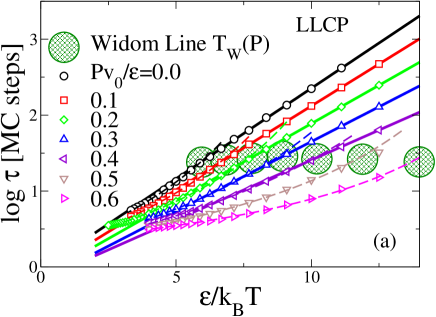
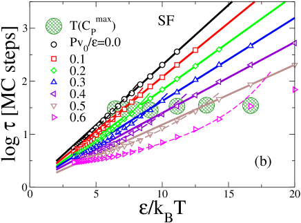
Figure 3: Dynamic crossover—large hatched circles of a radius approximately equal to the error bar—in the orientational relaxation time $\tau$ for a range of different pressures. (a) The LLCP scenario, with crossover temperature at $T_{W}(P)$. (b) The SF scenario, with crossover temperature at $T(C_{P}^{\rm max})$. Solid and dashed lines represent Arrhenius and VFT fits, respectively. Notice that the dynamic crossover occurs at approximately the same value of $\tau$ for all seven values of pressure studied.

For both scenarios we find a dynamic crossover (Fig. 3). At high $T$, we fit $\tau$ with the Vogel-Fulcher-Tamman (VFT) function

$$\tau^{\rm VFT}\equiv\tau_{0}^{\rm VFT}\exp\left[{T_{1}\over T-T_{0}}\right],$$ (5)

where $\tau_{0}^{\rm VFT}$, $T_{1}$, and $T_{0}$ are three fitting parameters. We find that $\tau$ has an Arrhenius $T$ dependence at low $T$, $\tau=\tau_{0}\exp[E_{\rm A}/k_{B}T]$, where $\tau_{0}$ is the relaxation time in the high-$T$ limit, and $E_{\rm A}$ is a $T$-independent activation energy. We find that for $J_{\sigma}/\epsilon=0.05$ the crossover occurs at $T_{W}(P)$ for $P<P_{C^{\prime}}$ [Fig. 3(a)], and that for $J_{\sigma}=0$ the crossover is at $T(C_{P}^{\rm max})$, the temperature of $C_{P}^{\rm max}$ [Fig. 3(b)]. We note that for both scenarios the crossover is isochronic, i.e. the value of the crossover time $\tau_{\rm C}$ is approximately independent of pressure. We find $\tau_{\rm C}\simeq 10^{3/2}$ MC steps.

We next calculate the Arrhenius activation energy $E_{\rm A}(P)$ from the low-$T$ slope of $\log\tau$ vs. $1/T$ [Fig. 4(a)]. We extrapolate the temperature $T_{\rm A}(P)$ at which $\tau$ reaches a fixed macroscopic time $\tau_{\rm A}\geq\tau_{\rm C}$. We choose $\tau_{\rm A}=10^{14}$ MC steps $>100$ sec kfbs06 [Fig. 4(b)]. We find that $E_{\rm A}(P)$ and $T_{\rm A}(P)$ decrease upon increasing $P$ in both scenarios, providing no distinction between the two interpretations. Instead, we find a dramatic difference in the $P$ dependence of the quantity $E_{\rm A}/(k_{B}T_{\rm A})$ in the two scenarios, increasing for the LLCP scenario and approximately constant for the SF scenario [Fig. 4(c)].

We can better understand our findings by developing an expression for $\tau$ in terms of thermodynamic quantities, which will then allow us to explicitly calculate $E_{\rm A}/(k_{B}T_{\rm A})$ for both scenarios. For any activated process, in which the relaxation from an initial state to a final state passes through an excited transition state, $\ln(\tau/\tau_{0})=\Delta(U+PV-TS)/(k_{B}T)$, where $\Delta(U+PV-TS)$ is the difference in free energy between the transition state and the initial state. Consistent with results from simulations and experiments Laage-Hynes2006 ; Tokmakoff , we propose that at low $T$ the mechanism to relax from a less structured state (lower tetrahedral order) to a more structured state (higher tetrahedral order) corresponds to the breaking of a bond and the simultaneous molecular reorientation for the formation of a new bond. The transition state is represented by the molecule with a broken bond and more tetrahedral IM order. Hence,

$$\Delta(U+PV-TS)=Jp_{\rm B}-J_{\sigma}p_{\rm IM}-Pv_{\rm B}-T\Delta S,$$ (6)

where $p_{\rm B}$ and $p_{\rm IM}$, the probability of a satisfied IM interaction, can be directly calculated. To estimate $\Delta S$, the increase of entropy due to the breaking of a bond, we use the mean field expression $\Delta S=k_{B}[\ln(2Np_{\rm B})-\ln(1+2N(1-p_{\rm B}))]\bar{p}_{\rm B}$, where $\bar{p}_{\rm B}$ is the average value of $p_{\rm B}$ above and below $T_{W}(P)$.

We next test that the expression of $\ln(\tau/\tau_{0})$, in terms of $\Delta S$ and Eq.(6),

$$\ln\frac{\tau}{\tau_{0}}=\frac{Jp_{\rm B}-J_{\sigma}p_{\rm IM}-Pv_{\rm B}}{k_{B}T}-\bar{p}_{\rm B}\ln\frac{2Np_{\rm B}}{1+2N(1-p_{\rm B})}$$ (7)

describes the simulations well, with minor corrections at high $T$. Here $\tau_{0}\equiv\tau_{0}(P)$ is a free fitting parameter equal to the relaxation time for $T\to\infty$. From Eq.(7) we find that the ratio $E_{\rm A}/(k_{B}T_{\rm A})$ calculated at low $T$ increases with $P$ for $J_{\sigma}/\epsilon=0.05$, while it is constant for $J_{\sigma}=0$, as from our simulations [Fig. 4(d)].

In summary, we have seen that both the LLCP and SF scenarios exhibit a dynamic crossover at a temperature close to $T(C_{P}^{\rm max})$, which decreases for increasing $P$. We interpret the dynamic crossover as a consequence of a local breaking and reorientation of the bonds for the formation of new and more tetrahedrally oriented bonds. Above $T(C_{P}^{\rm max})$, when $T$ decreases, the number of hydrogen bonds increases, giving rise to an increasing activation energy $E_{\rm A}$ and to a non-Arrhenius dynamics. As $T$ decreases, entropy must decrease. A major contributor to entropy is the orientational disorder, that is a function of $p_{\rm B}$, as described by the mean field expression for $\Delta S$. We find that, as $T$ decreases, $p_{\rm B}$ — hence the orientational order — increases. We find that the rate of increase has a maximum at $T(C_{P}^{\rm max})$, and as $T$ continues to decrease this rate drops rapidly to zero — meaning that for $T<T(C_{P}^{\rm max})$, the local orientational order rapidly becomes temperature-independent and the activation energy $E_{\rm A}$ also becomes approximately temperature-independent, for the Eq.(6). Corresponding to this fact the dynamics becomes approximately Arrhenius.

We find that the crossover is approximately isochronic (independent of the pressure) consistent with our calculations of an almost constant number of bonds at $T(C_{P}^{\rm max})$. In both scenarios, $E_{\rm A}$ and $T_{\rm A}$ decrease upon increasing $P$, but the $P$ dependence of the quantity $E_{\rm A}/(k_{B}T_{\rm A})$ has a dramatically different behavior in the two scenarios. For the LLCP scenario it increases as $P\to P_{C^{\prime}}$, while it is approximately constant in the SF scenario. We interpret this difference as a consequence of the larger increase of the rate of change of $p_{\rm B}$ in the LLCP scenario, where $p_{\rm B}$ diverges at finite $T_{C^{\prime}}$, compared to the SF scenario, where $p_{\rm B}$ can possibly diverge only at $T=0$. Since experiments can detect local changes of water structure from HDL-like to LDL-like, (e. g. Li05 ), it is possible that our prediction on the dynamic consequences of this local change may be experimentally testable.

We thank C. A. Angell, M.-C. Bellissent-Funel, W. Kob, L. Liu and S. Sastry for helpful discussions and NSF grant CHE0616489 for support. G. F. also thanks the Spanish Ministerio de Educación y Ciencia (Programa Ramón y Cajal and Grant No. FIS2004-03454).

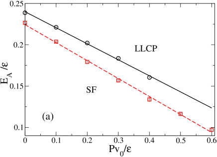
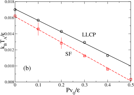
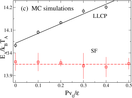
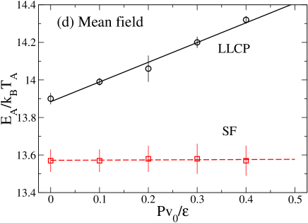
Figure 4: Effect of pressure on the activation energy $E_{\rm A}$. (a) Demonstration that $E_{\rm A}$ decreases linearly for increasing $P$ for both the LLCP and the SF scenarios. The lines are linear fits to the simulation results (symbols). (b) $T_{\rm A}$, defined such that $\tau(T_{\rm A})=10^{14}$ MC steps $>100$ sec kfbs06 , decreases linearly with $P$ for both scenarios. (c) $P$ dependence of the quantity $E_{\rm A}/(k_{B}T_{\rm A})$ is different in the two scenarios. In the LLCP scenario, $E_{\rm A}/(k_{B}T_{\rm A})$ increases with increasing $P$, and it is approximately constant in the SF scenario. The lines are guides to the eyes. (d) Demonstration that the same behavior is found using the mean field approximation. In all the panels, where not shown, the error bars are smaller than the symbol sizes.

References

- (1) C. A. Angell, Ann. Rev. Phys. Chem. 55, 559 (2004).
- (2) P. G. Debenedetti, J. Phys.: Condens. Matter 15, R1669 (2003).
- (3) P. H. Poole et al., Nature 360, 324 (1992).
- (4) S. Sastry et al., Phys. Rev. E 53, 6144 (1996); L. P. N. Rebelo et al., J. Chem. Phys. 109, 626 (1998).
- (5) G. D’Arrigo et al., J. Chem. Phys. 75, 4264 (1981); C. A. Angell and V. Rodgers ibid. 80, 6245 (1984).
- (6) A. K. Soper and M. A. Ricci, Phys. Rev. Lett. 84, 2881 (2000) and references cited therein. For simulations see E. Schwegler et al., Phys. Rev. Lett. 84, 2429 (2000); P. Raiteri et al., ibid. 93, 087801 (2004) and references cited therein.
- (7) G. Franzese and H. E. Stanley, Physica A 314, 508 (2002); J. Phys.: Cond. Mat. 14, 2193 (2002); G. Franzese et al., Phys. Rev. E. 67, 011103 (2003).
- (8) We find at , being somewhat smaller for increasing , consistent with the value 0.795 used in sdss to trace the temperature of maximum for . We find that for polynomial extrapolations of at up to the fifth order lead to a value of . Mean field calculations of compare well with simulations for and for .
- (9) P. Kumar et. al., Proc. Nat. Acad. Sci. 104, 9575 (2007).
- (10) L. Xu et al., Proc. Natl. Acad. Sci. 102, 16558 (2005); P. Kumar et al., Phys. Rev. Lett. 97, 177802 (2006).
- (11) Comparison with [P. Kumar et al., Phys. Rev. E 73, 041505 (2006)] shows that 1 MC step ps, the -relaxation time in supercooled water.
- (12) D. Laage and J. T. Hynes, Science 311, 832 (2006).
- (13) A. Tokmakoff, Science 317, 54 (2007) and references therein.
- (14) F. F. Li et al. J. Chem. Phys. 123, 174511 (2005).