Density-functional formulations for quantum chains

Abstract

We show that a lattice formulation of density-functional theory (DFT), guided by renormalization-group concepts, can be used to obtain numerical predictions of energy gaps, spin-density profiles, critical exponents, sound velocities, surface energies and conformal anomalies of spatially inhomogeneous quantum spin chains. To this end we (i) cast the formalism of DFT in the notation of quantum-spin chains, to make the powerful methods and concepts developed in ab initio DFT available to workers in this field; (ii) explore to what extent simple local approximations in the spirit of the local-density approximation (LDA), can be used to predict critical exponents and conformal anomalies of quantum spin models; (iii) propose and explore various nonlocal approximations, depending on the size of the system, or on its average density in addition to the local density. These nonlocal functionals turn out to be superior to LDA functionals.

I Introduction

In this work we show that a lattice formulation of density-functional theory (DFT), guided by renormalization-group concepts, can be used to obtain numerical predictions of energy gaps, spin-density profiles, critical exponents and conformal anomalies of spatially inhomogeneous quantum spin chains.

Density functional theory emerged over the years as an efficient and powerfull tool for electronic-structure theory in condensed matter physics, material science and quantum chemistry. In spite of these successful applications of DFT to continuum systems,kohnrmp ; dftbook DFT is not much used for interacting discrete systems, i.e., systems where the operators are defined on a lattice. Previous applications of DFT for discrete systems were to the one-dimensional Hubbard model describing electrons in solidsah1 ; ah2 ; ah3 ; ah4 ; ah5 or atoms in optical lattices,ah6 ; ah7 ; ah8 and to the Heisenberg spin-$\frac{1}{2}$ model in d-dimensions,ahe1 ; ahe2 ; ahe3 ; ahe4 employing local approximations similar to the local-density approximation (LDA) of ab initio electronic structure theory. The difficulty in treating such systems resides in the construction of a good functional. In Ref. ah3, , an LDA was constructed for the Hubbard model by exploiting the exact Bethe ansatz solution for the ground state of the infinite, spatially homogeneous, system. In Ref. ahe1, , LDA-like functionals for the Heisenberg model were obtained from an approximate spin-wave theory for the infinite homogeneous system, improved by adding numerical corrections from density-matrix renormalization-group calculations.

The purpose of this paper is to introduce a possible DFT formulation appropriate for general quantum chains, in particular near their quantum critical points. The construction of approximate density functionals exploits two seminal concepts from the theory of critical phenomena: the renormalization group and the conformal invariance of critical systems. From the renormalization group, it is known that the critical systems can be classified in universality classes. In each of these classes the low-energy physics is described by distinct homogeneous systems (fixed points) with correlation functions defined by appropriate critical exponents. Moreover, the underlying field theory describing most of these universality classes is conformally invariant. This symmetry classifies these classes by the conformal anomaly $c$, or the central charge of the conformal algebra, and the critical exponents are given in terms of the highest weights representations of this algebra.BPZ These facts lead us to expect that a single density functional could describe the whole family of critical models of a given universality class of critical behavior. In principle, the construction of such functionals can proceed by exploiting the exact results provided along the years by the Bethe ansatzbethe in its several formulations.

It is believed that for each universality class of critical behavior there is at least one exactly integrable quantum chain. The exact solution of that quantum chain underlies the construction of the functional for several models belonging to the universality class. In order to test this general idea we restrict ourselves to one of the most important universality classes of critical behavior, namely, the $c=1$ conformal invariant models, with continuously varying critical exponents. Models in this universality class are the Gaussian model,gaussian the anisotropic antiferromagnetic Heisenberg model with half-odd integer spin,ab2 ; alc-moreo the ferromagnetic version of the exact integrable Taktajan-Babujian models,alc-martins the anisotropic biquadratic spin $1$ chain,biqua the Ashkin-Teller quantum chain,ab2 etc.

As a representative of this class of models we are going to consider the exactly integrable spin-$\frac{1}{2}$ anisotropic Heisenberg model or the XXZ quantum chain. This model is considered a paradigm of integrability, and its critical exponents are known exactly.

Due to the conformal invariance, the leading finite-size corrections of the eigenenergies of the quantum chains are ruled by the conformal anomaly and the critical exponents of the critical chains.anomaly ; cardy The exact knowledge of the ground state energy in the bulk limit and in the finite geometry will allow us to construct good LDA approximations for the functionals. Some of these LDAs will be good enough to reproduce the exact values of the conformal anomaly and critical exponents. Such LDA approximations, although applied in this paper only to the XXZ chain, reveal interesting general features, that certainly will be helpful for other discrete quantum systems. Our analysis reveals the essential ingredients and the degree of accuracy we should demand from a density functional to obtain from it reliable results for the conformal anomaly and critical exponents.

Once such a functional is available, numerical analysis of complex Hamiltonians is greatly simplified. As an example, in the case we are mainly concerned with below, the XXZ chain, full exact diagonalization becomes hard for more than $\approx 12$ sites, Lanczos methods allow one to reach about three times as much, whereas density-functional techniques can still be applied for systems with thousands of sites, even if translational invariance is broken.

The layout of this papers is as follows. In Sec. II we give an introduction to the general framework of DFT for spin chains (Sec. II.1) and to local approximations that make this framework useful in practice (Sec. II.2). In Sec. III we then describe the representative spin chain we are mainly concerned with in this work: the XXZ model. Section IV is devoted to the construction of local approximations for the XXZ chain, and an exploration of their performance for systems with periodic (Sec. IV.1), twisted (Sec. IV.2) and open (Sec. IV.3) boundary conditions. In Sec. V we then go beyond local approximations, and construct nonlocal functionals (Sec. V.1), which are applied to systems with open boundary conditions (Sec. V.2) and in the presence of spatially varying magnetic fields (Sec. V.3). Section VI contains our conclusions.

II Density-functional approach to quantum spin chains

II.1 General aspects of DFT for quantum spin chains

Density-functional theory is a formally exact way to cast the many-body problem in terms of densities instead of wave functions. For a large class of Hamiltonians — characterized by a stable ground state and containing a density-like intensive variable coupled to an external field — the fundamental Hohenberg-Kohn theorem shows that the density variable determines the ground state wave function, which implies that all ground state observables are functionals of the density.kohnrmp ; dftbook

This general theorem does not tell one how to obtain these functionals, how to calculate the density, what the physical nature of the external field is — and not even how to select the density variable in the first place. All of these questions must be answered before applying DFT to a specific class of problems. Here we attempt to do this for a large family of spin Hamiltonians, by combining concepts from DFT with renormalization-group ideas.

In practice, the density variable is typically chosen to represent the charge or spin distribution in a continuous space or on a lattice. The ground state energy becomes a functional of this distribution, which is minimized to provide the ground state density. Of course, the energy functional is not known exactly for nontrivial many-body systems. Successful approximation schemes are based on the local-density concept, which takes as an input the ground state energy of a spatially homogeneous system, in which the density distribution is uniform. The corresponding energy density is then evaluated point by point at the actual densities of the inhomogeneous system under study.

While this means that DFT in the local-density approximation (LDA) requires as an input a good solution to the spatial homogeneous system (which in itself may be hard to obtain), it also implies that once that solution is avaliable, the LDA can be used to obtain approximations to the ground state energy and density distributions of inhomogeneous systems. In ab initio applications of DFT, the homogeneous system is the electron liquid, the external potential is produced by the nuclei, and the resulting inhomogeneous systems are atoms, molecules and solids.kohnrmp ; dftbook

For model Hamiltonians defined on lattices, the homogeneous system is one in which all sites are equivalent, and inhomogeneous systems can have boundaries, impurities, confining potentials, or other translation-symmetry breaking terms. Since model Hamiltonians are typically much better controlled than the ab initio one, much more information is available for constructing the LDA and for testing its predictions. This additional information provides a two-pronged opportunity: (i) Learn about inhomogeneous model Hamiltonians, which have too few symmetries to be integrable and require too large matrices to be numerically diagonalizable, by means of LDA calculations. (ii) Learn about DFT, the LDA, and its improvements, by studying them in the context of model Hamiltonians. Here we explore both aspects for spin Hamiltonians, and inquire, in particular, if and how LDA-type functionals can be used to predict the critical exponents and conformal anomalies associated with the quantum critical points of these Hamiltonians.

II.2 Local density functionals for quantum spin chains

The family of quantum chains for which we are going to seek a DFT formulation, describes quantum spin operators attached to $L$ sites ($i=1,\ldots,L$) of a one dimensional lattice, with Hamiltonian

$$H=H_{0}+V^{\mbox{\scriptsize ext}}.$$ (1)

The operator $H_{0}$ may contain, e.g., the kinetic energy operator and the static interaction energy among the spins on distinct sites, while $V^{\mbox{\scriptsize ext}}$ is the on-site potential.

Here, we consider Hamiltonians of the form (1) that commute with the global charge $\hat{N}=\sum_{i=1}^{L}\hat{n}_{i}$, whose eigenvalues take a discrete set of values ($N=0,1,2,\ldots$). Moreover the on-site potential in (1) is a function of the local density operators $\hat{n}_{i}$, having the general form

$$V^{\mbox{\scriptsize ext}}=\sum_{i=1}^{L}v_{i}^{\mbox{\scriptsize ext}}\hat{n}_{i},$$ (2)

where $v_{i}^{\mbox{\scriptsize ext}}$ ($i=1,\ldots,L$) are arbitrary site-dependent couplings that fix the profile of the spacial inhomogeneities of the quantum chain. Examples of models in this family are the spin $S$ Heisenberg models, where $\hat{N}$ is related to the $S^{z}$-magnetization, and the Hubbardlieb-wu and t-J models, where $\hat{N}$ is related to the number of fermions.

For this class of models we can separate the Hilbert space associated to (1) into block disjoint sectors labelled by the eigenvalues $N=0,1,2,\ldots$. The variational principle, restricted to a given sector of total charge $N=\sum_{i=1}^{L}n_{i}$, give us the lowest eigenenergy on the sector

$$E_{0}=\mbox{min}_{|\Psi>}<\Psi^{(N)}|H|\Psi^{(N)}>=<\Psi_{0}^{(N)}|H|\Psi_{0}^{(N)}>,$$ (3)

where $|\Psi^{(N)}_{0}>$ is the eigenfunction corresponding to this lowest eigenenergy.

The minimization procedure of (3) can be done conveniently in two steps by following the constrained-search approach of Levylevy and Lieb.lieb In the first step we consider, for a given density distribution $n_{i}$ ($i=1,\ldots,L$), restricted to $\sum_{i=1}^{L}n_{i}=N$, the ensemble of states $\{|\Psi>\}_{n_{1},\ldots,n_{L}}$ such that $<\Psi|\hat{n}_{i}|\Psi>=n_{i}$ ($i=1,\ldots,L$). On this ensemble we minimize $<\Psi|H|\Psi>$, i.e.,

$$\mbox{min}_{|\Psi>_{n_{1},\ldots,n_{L}}}<\Psi|H|\Psi>=F_{I}[n]+\sum_{i=1}^{L}v_{i}^{\mbox{\scriptsize ext}}n_{i},$$ (4)

where the special form of (2) was used, and

$$F_{I}[n]=\mbox{min}_{|\Psi>_{n_{1},\ldots,n_{L}}}<\Psi|H_{0}|\Psi>$$ (5)

is in general a functional of the density $n$. On a lattice, $F_{I}[n]$ reduces to a function of the $L$ independent variables $n_{1},\ldots,n_{L}$, but for consistency with the ab initio literature we continue to employ the expression ’functional’. For notational convenience, we below frequently employ $n$ in the argument of a functional, i.e., between square brackets, to denote the entire discrete distribution of values $n_{1},\ldots,n_{L}$. When used on its own, or as an argument of a simple function of one variable, $n$ represents just one value, which can be site dependent ($n_{i}$) or constant ($n=N/L$).

In the second step we minimize (4) over all densities satisfying $\sum_{i=1}^{L}n_{i}=N$, i.e.,

$$\delta\left[F_{I}[n]-\sum_{i=1}^{L}v_{i}^{\mbox{\scriptsize ext}}n_{i}-\mu\sum_{i=1}^{L}n_{i}\right]=0,$$ (6)

where $\mu$ is a Lagrange multiplier and plays the role of a chemical potential. We have then reduced the variational problem (3) to (5) and (6). Unless we have a good approximation for $F_{I}[n]$, this procedure is, of course, purely formal.

In order to proceed, we now suppose that we can define a simple Hamiltonian $H_{0}^{s}$ acting on the same Hilbert space as (1) and having the following three properties. (i) It has the same global symmetries as $H_{0}$ in (1). (ii) We are able to calculate its ground state even in the presence of external inhomogeneous on-site potentials of the type given in (2), where the Hamiltonian is given by

$$H_{s}=H_{0}^{s}+\sum_{i=1}^{L}v_{i}^{s}\hat{n}_{i},$$ (7)

with $v_{i}^{s}$ ($i=1,\ldots,L$) arbitrary. (iii) There exists a special choice of $v_{i}^{s}$ ($i=1,\ldots,L$) such that the ground state of (7) has the same density $\{n_{i}\}$ as the ground state of the nontrivial interacting Hamiltonian (1). The auxiliary Hamiltonian $H_{s}$ is the Kohn-Sham Hamiltonian of DFT. It is not intended to approximate the complex problem posed by the Hamiltonian $H$, but to obtain the ground state densities and energies of $H$.kohnrmp ; dftbook

Property (i) is not rigorously necessary, but it simplifies our analysis without too much restricting its generality. It allows us to consider $H_{s}$ on the sectors labelled by the eigenvalues $N=0,1,2,\ldots$ of the commuting operator $\hat{N}$. Property (ii) is needed to make the formulation practical, as it ensures that we can calculate the ground state energy and density of the simpler Hamiltonian (7). Property (iii) is equivalent to a v-representability assumption,dftbook and is essential for the procedure to work.

Given these three properties, we can use the variational procedure (3)-(6) to obtain the ground state energy from the minimization

$$\delta\left[F_{s}[n]-\sum_{i=1}^{L}v_{i}^{s}n_{i}-\mu^{s}\sum_{i=1}^{L}n_{i}\right]=0,$$ (8)

where, as in (5),

$$F_{s}[n]=\mbox{min}_{|\Psi>_{n_{1},\ldots,n_{L}}}<\Psi|H_{0}^{s}|\Psi>,$$ (9)

and $\mu^{s}$ is a Lagrange multiplier. Comparison of (8) and (6) implies that the density profile ($n_{1},\ldots,n_{L}$) corresponding to the ground state of the complicated Hamiltonian (1) is the same as that of the ground state of the simple Hamiltonian $H_{s}$, provide we choose

$$\sum_{i=1}^{L}v_{i}^{s}n_{i}=\sum_{i=1}^{L}v_{i}^{\mbox{\scriptsize ext}}n_{i}+W[n]+(\mu-\mu^{s})N,$$ (10)

where

$$W[n]=F_{I}[n]-F_{s}[n].$$ (11)

This implies

$$v_{i}^{s}=v_{i}^{\mbox{\scriptsize ext}}+\frac{\partial W[n]}{\partial n_{i}}+\mu-\mu^{s}.$$ (12)

For a given site $i$, the potential $v_{i}^{s}$ depends on the entire distribution of local densities $n_{1},\ldots,n_{L}$. We have then to solve (7) selfconsistently for the ground state energy $E_{s}$ and the corresponding densities $\{n_{1},\ldots,n_{L}\}$. The difference $\mu-\mu^{s}$ in (10) and (12) is just a harmless constant in the above selfconsistent procedure, since we are always in a sector with a fixed value of $N$, and hence we may choose $\mu=\mu^{s}$. As a consequence of (10) and (3)-(5), the ground state energy of the complicated Hamiltonian (1) is

$$E[n]=E_{s}[n]-\sum_{i=1}^{L}\frac{\partial W[n]}{\partial n_{i}}n_{i}+W[n],$$ (13)

which can be calculated once the density is known.

The success of this DFT formulation will depend on our ability to produce good approximations for $W[n]$. In ab initio DFT, the functional $F_{s}$ is just the kinetic energy $T_{s}$ of the noninteracting Hamiltonian $H_{s}$, and the functional $F_{I}[n]$ is decomposed asdftbook

$$F_{I}[n]=T_{s}[n]+E_{H}[n]+E_{xc}[n],$$ (14)

where $E_{H}$ is the Hartree energy (the mean-field approximation to the Coulomb interaction energy) and $E_{xc}$ the exchange-correlation energy. $E_{xc}$ is unknown, and must be approximated. $E_{H}$ is known explicitly, and $T_{s}$, although not known explicitly as a density functional, is easily obtained from solving the Hamiltonian $H_{s}$. For general model Hamiltonians, the various terms in $F_{I}$ need not have the same physical interpretation. We therefore simply write $F_{I}[n]=F_{s}[n]+W[n]$, as above, and develop approximations for $W[n]$.

If $F_{I}$ contains pieces that are known exactly, it is advantageous to treat these separately, and approximate only the remainder (e.g., $E_{xc}$ in the ab initio case). A typical case is the mean-field approximation to the interaction energy, leading to a Hartree-like contribution to $W$. Below we develop local approximations to $W[n]$, but in the models we are concerned with the Hartree term itself is local, so that nothing is gained by giving it special treatment at this stage.

In order to turn the formulation into a practical tool, we require approximate expressions for $W[n]$ that keep the essential ingredients of the exact unknown functional. A general prescription for systematically producing such approximations is to split the functional $W[n]$ into $L$ identical parts, according to

$$W(n_{1},\ldots,n_{L})=\sum_{i=1}^{L}w_{i}$$ (15)

where

$$w_{i}\equiv\frac{W(n_{1},\ldots,n_{L})}{L},\;\;i=1,\ldots,L.$$ (16)

We now expand, for a given inhomogeneous distribution $n_{1},\ldots,n_{L}$, each of the $L$ terms $w_{i}$ around a distinct homogeneous distribution,

$$w_{i} = \frac{W(n_{i},\ldots,n_{i})}{L}+\sum_{j=1}^{L}\alpha_{j}[n_{i}](n_{j}-n_{i})$$ (17)

$$+ \sum_{j=1}^{L}\sum_{l=1}^{L}\beta_{j,l}[n_{i}](n_{j}-n_{i})(n_{l}-n_{i})+\cdots.$$

The i’th term is thus expanded around a homogeneous distribution in which all sites have the density $n_{i}$ of the i’th site in the inhomogeneous distribution. Here $\alpha_{j}[n_{i}]$ and $\beta_{j,l}[n]$ depend on the local densities,

$$\alpha_{j}[n_{i}] = \frac{1}{L}\frac{\partial W(n_{1},\ldots,n_{L})}{\partial n_{j}}{\Bigg{|}}_{n_{1}=\cdots=n_{L}=n_{i}},$$

$$\beta_{j,l}[n_{i}] = \frac{1}{2L}\frac{\partial^{2}W}{\partial n_{i}\partial n_{l}}{\Bigg{|}}_{n_{1}=\cdots=n_{L}=n_{i}}.$$ (18)

The first term in this expansion provides a local density approximation (LDA) to the functionals. The second and higher-order terms yield non-local contributions similar to those obtained in gradient expansions of the density functional for Coulomb-interacting electronic systems.

Most of our analysis in the next sections is based on the LDA, i.e., the first term in (17)

$$W^{\mbox{\scriptsize LDA}}(n_{1},\ldots,n_{L})=\sum_{i=1}^{L}\frac{W(n_{i},n_{i},\ldots,n_{i})}{L}.$$ (19)

The exact functional $W$ evaluated at an infinite and homogeneous density distribution $n_{1}=\cdots=n_{L}=n_{i}$, reduces to the functional of the infinite homogeneous system, depending only on the variable $n_{i}$, whose value per site we denote as $w^{\infty}(n)$. The LDA then assumes the more familiar form

$$W^{\mbox{\scriptsize LDA},\infty}(n_{1},\ldots,n_{L})=\sum_{i=1}^{L}w^{\infty}(n)|_{n=n_{i}}.$$ (20)

To compare this with the LDA in use in electronic-structure theory, recall that there the Hartree term is nonlocal, and the local approximation is only applied to the difference $E_{xc}=F_{I}-F_{s}-E_{H}$, whereas here we apply it directly to $W=F_{I}-F_{s}$.

In this paper we explore the possibility to obtain the critical exponents and conformal anomaly of critical Hamiltonians, by means of simple functionals constructed following the above prescription. As a consequence of conformal invariance,cardy these quantities are obtained from the amplitudes of the $O(1/L^{2})$ finite-size corrections of the energies per site of the quantum chains of size $L$. A finite-size quantum chain can still be homogeneous, if all sites have the same spin, and periodic boundary conditions are applied. Although the LDA becomes exact in the infinite homogeneous system, in a finite homogeneous system it will have an additional error. If such error is of $O(1/L^{2})$, we are going to obtain wrong critical exponents.

An improvement is obtained by using the ground state energy per site of a translationally invariant Hamiltonian with $L$ sites, instead of that of the infinite system. In this case the functional depends on the size $L$ of the system, and can be written as

$$W^{\mbox{\scriptsize LDA,L}}(n_{1},\ldots,n_{L})=\sum_{i=1}^{L}w^{(L)}(n)|_{n=n_{i}},$$ (21)

where $e^{(L)}(n_{i})$ is the ground state energy per site of the Hamiltonian $H_{0}$.

Note that this LDA-like expression is not, strictly speaking, a local functional, as it depends on the size of the system (i.e., the number of elements in the set $\{n_{1}\ldots n_{L}\}$), which is a highly nonlocal function of $n_{i}$. The resulting effective magnetic field $h_{i}^{s}$ at site $i$ does not depend only on the density at that site (as it does in local approximations), but on the number of sites. In applications reported below, this nonlocality endows the functional with superior properties, compared to the usual LDA. In spite of this nonlocality, we call this latter functional the finite-size LDA, because of its conceptual similarity with the usual (infinite-size) LDA, deriving from the thermodynamic limit. A different type of nonlocality is explored in Sec. V.

Both local-density approximations, (20) and (21), as well as the gradient expansion (15)-(II.2), are applicable to very general classes of model Hamiltonians. In the remainder of this paper, we employ concepts arising in the context of the renormalization group, in order to exemplify and test these approximations. The concept of universality classes of models near criticality allows us to consider one representative of critical quantum spin chains, and deduce from it results expected to be valid for the entire class. Specifically, we use the LDAs (20) and (21) to obtain the energies of the XXZ chain and test the possibility of obtaining the conformal anomaly and critical exponents from LDA. The conformal invariance of the model allows us to obtain predictions for these quantities from energies of finite chains. (Later on, in Sec. V, conformal invariance is used not only to extract information from functionals, but also to construct nonlocal approximations.) For Kohn-Sham Hamiltonians that belong to the same universality class as the interacting Hamiltonians, universality guarantees that LDA critical exponents are given correctly. Nonuniversal quantities, such as the sound velocity, are predicted wrongly by some forms of LDA, but a suitable rescaling of the Hamiltonian can be used to cure this defect.

III The XXZ quantum chain

Critical quantum chains belonging to the same universality class have the same critical exponents and, in the case of conformally invariant systems, the same conformal anomaly $c$. We expect that density functionals for such systems will share the same general features. In this section we consider the universality class comprising the $c=1$ conformally invariant quantum chains. These quantum chains exhibit a critical line with continuously varying critical exponents. The underlying field theory describing the long-distance physics of such models is the Gaussian model (or Coulomb gas).gaussian This field theory is described by operators $\Phi_{n,m}$ composed of a spin-wave excitation index $n$ and a ”vortex” excitation of vorticity $m$. The anomalous dimensions of these operators, related to the critical exponents of the quantum chain, are given by

$$x_{n,m}=n^{2}x+\frac{m^{2}}{4x},\;\;\;n,m=0,\pm 1,\pm 2,\ldots.$$ (22)

The parameter $x$ varies continuously along the critical line and its value depends on the interactions entering the particular model.gaussian-note Examples of models exhibiting such critical behavior are the anisotropic spin-$S$ Heisenberg model,alc-moreo the Ashkin-Teller model,ab2 the anisotropic triplet spin model introduced in Ref. alc-barber, , the ferromagnetic spin-$S$ Babujian-Taktajan models,alc-martins the anisotropic biquadratic spin $1$ chain,biqua etc.

The most studied model in this family of $c=1$ models is the anisotropic spin-$\frac{1}{2}$ Heisenberg chain, also known as the XXZ chain, whose Hamiltonian is given by

$$H^{\mbox{\scriptsize XXZ}}(\Delta)=-\frac{1}{2}\sum_{j=1}^{L}(\sigma_{j}^{x}\sigma_{j+1}^{x}+\sigma_{j}^{y}\sigma_{j+1}^{y}+\Delta\sigma_{j}^{z}\sigma_{j+1}^{z}).$$ (23)

Here $\vec{\sigma}\equiv(\sigma^{x},\sigma^{y},\sigma^{z})$ are Pauli matrices, $L$ is the lattice size and $\Delta$ is the anisotropy, which in the DFT framework plays the role of a spin-spin interaction. This Hamiltonian is exactly integrable through the Bethe ansatz.yang-yang Its exact solution shows that, in the bulk limit $L\rightarrow\infty$, the model is critical (gapless) for anisotropies $-1\leq\Delta=-\cos\gamma\leq 1$. As a consequence of the conformal invariance of the model, the critical exponents are exactly given by Eq (22),ab2 ; hamer with the model dependent parameter $x=x_{\Delta}$ given by

$$x_{\Delta}=\frac{\pi-\gamma}{2\pi},\;\;\;\Delta=-\cos\gamma,\;\;0\leq\gamma\leq\pi.$$ (24)

The XXZ quantum chain is then a natural candidate to develop approximate functionals for DFT applications to critical models in the $c=1$ universality class. The exactly known finite-size corrections of the modelab2 will allow us to test the general ideas presented in Sec. II.

As in Sec. II.2, we consider a non integrable generalization of (23) where besides the intersite spin-spin interactions we also include the on-site interactions of the spins with an inhomogeneous site-dependent external magnetic field $h_{i}^{\mbox{\scriptsize ext}}$ ($i=1,\ldots,L$), namely,

$$H^{\mbox{\scriptsize XXZ}}(\Delta,\{h_{i}\})=H_{0}^{\mbox{\scriptsize XXZ}}(\Delta)+V^{\mbox{\scriptsize ext}}$$

$$=\frac{1}{2}\sum_{j=1}^{L}(\sigma_{j}^{x}\sigma_{j+1}^{x}+\sigma_{j}^{y}\sigma_{j+1}^{y}+\Delta\sigma_{j}^{z}\sigma_{j+1}^{z})$$

$$-\frac{1}{2}\sum_{j=1}^{L}h_{j}^{\mbox{\scriptsize ext}}(\sigma_{j}^{z}+1),$$ (25)

where we added a convenient constant. In this paper we study the Hamiltonian (III) with several types of boundary conditions. For periodic ($p=1$) and open boundary conditions ($p=0$) we have

$$\vec{\sigma}_{L+1}=p\vec{\sigma}_{1},\;\;\;p=0,1,$$ (26)

whereas for twisted boundary conditions

$${\sigma^{\pm}}_{L+1}=e^{\pm i\phi}{\sigma}^{\pm}_{1},\;\;\;\sigma_{L+1}^{z}=\sigma_{1}^{z},$$ (27)

where $0\leq\phi\leq 2\pi$ and $\sigma^{\pm}=\frac{1}{2}(\sigma^{x}\pm i\sigma^{y})$ are the usual raising and lowering $SU(2)$ spin operators.

The inhomogeneous Hamiltonian (III) is suitable for the DFT approach presented in Sec. II. It has a $U(1)$ symmetry, and it is easy to obtain a simple Hamiltonian $H^{s}$, as in (7), with the properties (i)-(iii) discussed in Sec. II. The Hamiltonian (III) commutes with the global charge

$$\hat{N}=\sum_{i=1}^{L}\hat{n}_{i},\;\;\;\hat{n}_{i}=\frac{\sigma_{i}^{z}+1}{2},\;\;i=1,\ldots,L,$$ (28)

which gives the total number of up spins in the $\sigma^{z}$-basis. By comparing (1), (2) and (III) we identify

$$V^{\mbox{\scriptsize ext}}=\sum_{i=1}^{L}v_{i}^{\mbox{\scriptsize ext}}\hat{n}_{i},\;\;\;v_{i}^{\mbox{\scriptsize ext}}=-h_{i},\;\;\;\ i=1,\ldots,L.$$ (29)

The simple Hamiltonian that plays the role of the Kohn-Sham Hamiltonian is obtained by setting $\Delta=0$ in (III), i.e.,

$$H_{s}(\{h_{i}^{s}\})=H^{\mbox{\scriptsize XXZ}}(\Delta=0,\{h_{i}^{s}\})=H^{\mbox{\scriptsize XXZ}}(0)-\sum_{i=1}^{L}h_{i}^{s}\hat{n}_{i}.$$ (30)

This simple Hamiltonian is the well known XY model in the presence of site-dependent magnetic fields $h_{i}^{s}$ ($i=1,\ldots,L$). Through a Jordan-Wigner transformationjordan-wigner $H_{s}$ is tranformed into a Hamiltonian describing $L$ non-interacting spinless fermions. The $2^{L}$ eigenenergies of $H_{s}$ are given by arbitrary combinations of free fermion energies, given in terms of the eigenvalues of a $L\times L$ matrix, whose elements depend on the boundary condition in (30) and the values of the magnetic fields $h_{i}^{s}$ ($i=1,\ldots,L$). This implies that with reasonable computing efforts we can diagonalize $H_{s}$ for lattice sizes up to $L=L_{\mbox{\scriptsize max}}\approx 5000$. This is certainly much more we could reach for the $2^{L}\times 2^{L}$ interacting Hamiltonian (III).

The inhomogeneous magnetic field $h_{i}^{s}$ ($i=1,\ldots,L$) are fixed, as in (12), by imposing that the ground state eigenfunction of (30) and (III), on a given sector with fixed number $N$ of up spins, share the same density distribution $n_{i}$ ($i=1,\ldots,L$) of up spins:

$$h_{i}^{s}=h_{i}^{\mbox{\scriptsize ext}}-\frac{\partial W[n]}{\partial n},\;\;\;\ i=1,\ldots,L.$$ (31)

As in (33), $W[n]$ is given by the difference of the functionals of the interacting (5) and non-interacting (9) models. Since in the present case $H_{s}$ is obtained from $H$ by setting $\Delta=0$, the corresponding functionals are related and we can write

$$W[n]=F_{\Delta}[n]-F_{\Delta=0}[n],$$ (32)

where $F_{\Delta}$ is the functional obtained by using in (5) the Hamiltonian $H^{\mbox{\scriptsize XXZ}}(\Delta)$ given in (23), i.e.,

$$F_{\Delta}[n]=\mbox{min}_{|\Psi>_{n_{1},\ldots,n_{L}}}<\Psi|H^{\mbox{\scriptsize XXZ}}(\Delta)|\Psi>.$$ (33)

The density profile $n^{0}=(n_{1}^{0},\ldots,n_{L}^{0})$ of the ground state of $H^{\mbox{\scriptsize XXZ}}(\Delta,\{h_{i}\})$ restricted to the sector with $N$ up spins, is obtained by solving self-consistently (30) with (31). From (13) the ground state energy of the inhomogeneous interacting model (III) is given by

$$E_{N}=E[n^{0}]=E_{s}(\{h_{i}^{s}\})-\sum_{i=1}^{L}\frac{\partial W[n^{0}]}{\partial n_{i}^{0}}n_{i}^{0}+W[n^{0}].$$ (34)

Here $E_{s}(\{h_{i}^{s}\})$ is the ground state energy of the free fermion XY Hamiltonian $H^{\mbox{\scriptsize XXZ}}(\Delta=0,\{h_{i}^{s}\})$, with $N=\sum_{i=1}^{L}n_{i}^{0}$ up spins.

All difficulties in obtaining the energies $E_{N}$ in (34) now reduce to the derivation of the functional $W_{\Delta}[n]$ in (32). Following the approximations considered in Sec. II, we next consider the XXZ chain with distinct boundary conditions and inhomogeneities.

IV Local approximations for the XXZ chain

In the absence of external fields $h_{i}$, the only source of inhomogeneity (i.e., breaking of translational invariance) are the boundaries. In this section we consider the Hamiltonian (23) on finite chains, for periodic, twisted and open boundary conditions.

IV.1 Periodic boundary conditions

In this case, beyond the conservation of the total number of up spins, the Hamiltonian (23) is also translationally invariant. As a consequence, we can separate the Hilbert space associated with the interacting model $H^{\mbox{\scriptsize XXZ}}(\Delta)$, as well as that of the auxiliary Kohn-Sham Hamiltonian $H^{\mbox{\scriptsize XXZ}}(\Delta=0)$, into block-disjoint sectors labelled by the density of up spins $n=\frac{N}{L}$, ($n=0,\frac{1}{L},\frac{2}{L},\ldots,1$) and momentum $p=\frac{2\pi}{L}j$ ($j=0,1,\ldots,L-1$). In each of these sectors we can apply the DFT-LDA procedure of section II to calculate the lowest energy $E_{0}(L,n,p)$.

Let $|\phi>$ be any vector on the arbitrary sector ($n,p$), i.e., $\sum_{i=1}^{L}{\hat{n}}_{i}/L|\phi>=n|\phi>$ and $\hat{T}|\phi>=e^{ip}|\phi>$, where $\hat{T}$ is the translation operator. It is simple to show that

$$n_{i}=\frac{<\phi|\hat{n}_{i}|\phi>}{<\phi|\phi>}=\frac{\sum_{i=1}^{L}n_{i}}{L}=\frac{N}{L}=n,\;\;\;i=1,\ldots,L.$$ (35)

This implies that any eigenvector of $H^{\mbox{\scriptsize XXZ}}(\Delta)$ has a uniform distribution of densities $n_{i}=n$ ($i=1,\ldots,L$).

The functional $F_{\Delta}[n,p]=F_{\Delta}(n,p)$, for general values of $\Delta$, is in the present case a simple function of the two variables $n=N/L$ and $p$. Consequently the local magnetic fields $\{h_{i}^{s}\}$ in the auxiliary Hamiltonian (30) are site independent:

$$h_{i}^{s}=-\frac{dW_{\Delta}(n,p)}{dn}=-\frac{d}{dn}(F_{\Delta}(n,p)-F_{0}(n,p))\equiv h^{s}.$$ (36)

$H_{s}(\{h_{i}^{s}\})$, in this case, is just the XY model in the presence of a uniform magnetic field $h_{s}$. The lowest energy of this auxiliary Hamiltonian, in the sector $(n,p)$, is given by

$$E_{s}(h^{s})=Le^{L,\mbox{\scriptsize per}}_{\Delta=0}(n,p)-Lh^{s}n,$$ (37)

where $e^{L,\mbox{\scriptsize per}}_{\Delta=0}(n,p)=e^{L,\mbox{\scriptsize per}}_{0}(n,p)$ is the lowest eigenenergy per site in the sector $(n,p)$ of the XY model in the absence of external magnetic fields.

In order to obtain the lowest eigenenergies of the interacting model on the sector $(n,p)$, from (34), it is necessary to know the functional $W_{\Delta}(n,p)$. Following the discussions of Sec. III, we use the local approximations (20) and (21) for this functional. In the present case they are given by

$$W_{\Delta}^{\mbox{\scriptsize LDA},L}(n,p)=\sum_{i=1}^{L}w_{\Delta}^{L,\mbox{\scriptsize per}}(n,p)=Lw_{\Delta}^{L,\mbox{\scriptsize per}}(n,p),$$ (38)

$$W_{\Delta}^{\mbox{\scriptsize LDA},\infty}(n,p)=\sum_{i=1}^{L}w_{\Delta}^{\infty}(n,p)=Lw_{\Delta}^{\infty}(n,p).$$ (39)

Here $w_{\Delta}^{L,\mbox{\scriptsize per}}(n,p)=e_{\Delta}^{L,\mbox{\scriptsize per}}(n,p)-e_{0}^{L,\mbox{\scriptsize per}}(n,p)$ and $w_{\Delta}^{\infty}(n,p)=e_{\Delta}^{\infty}(n,p)-e_{0}^{\infty}(n,p)$ are the interaction energies per site, and $e_{\Delta}^{L,\mbox{\scriptsize per}}(n,p)$ and $e_{\Delta}^{\infty}(n,p)$ represent the lowest total energy per site in the sector $(n,p)$ of the periodic Hamiltonian $H^{\mbox{\scriptsize XXZ}}(\Delta,p)$ with $L$ sites and with an infinite number of sites, respectively. The Hamiltonian $H^{\mbox{\scriptsize XXZ}}(\Delta,0)$, with periodic boundaries, is exactly integrable through the Bethe ansatz.yang-yang The eigenenergies for lattice size $L$, are obtained by solving a set of $N=nL$ coupled non-linear equations. This can be done,ab2 at least for the lower eigenenergies of sectors $(n,p)$, either for lattice sizes up to $L\approx 1000$ or in the bulk limit ($L\rightarrow\infty$).

Suppose, for the moment, that we have evaluated exactly $e_{\Delta}^{L,\mbox{\scriptsize per}}(n,p)$ and the LDA functional (38) and (39). The lowest eigenenergy, in the sector $(n,p)$, is obtained by inserting (37) in (34) and using one of the approximations (38) or (39). From the finite-size LDA functional (38) we obtain

$$E_{\Delta}^{\mbox{\scriptsize LDA},L}(L,n,p)=Le^{L,\mbox{\scriptsize per}}_{0}(n,p)-Lh^{s}n$$

$$-\sum_{i=1}^{L}n\frac{\partial W_{\Delta}(n,p)}{\partial n}+W_{\Delta}(n,p).$$ (40)

The relation (36) gives, in this case, the exact result

$$E_{0}^{\mbox{\scriptsize LDA},L}(L,n,p)=Le_{\Delta}^{L,\mbox{\scriptsize per}}(n,p).$$ (41)

This result is expected, since the density distribution of up spins for any of the eigenlevels is spatially homogeneous, and we only need to keep the first term in the expansion (15)-(II.2). The conformal anomaly and critical exponents that are calculated from the leading finite-size corrections of the eigenenergies, are then obtained exactly.

This is not the case for the LDA functional (39), which derives from the infinite chain. If we use (39) and (37) in (34), we obtain

$$E_{\Delta}^{\mbox{\scriptsize LDA},\infty}(L,n,p)=Le_{0}^{L,\mbox{\scriptsize per}}(n,p)-Lh^{s}n$$

$$-\sum_{i=1}^{L}[\frac{\partial}{\partial n}(e_{\Delta}^{\infty}(n,p)-e_{0}^{\infty}(n,p))]n$$

$$+L(e_{\Delta}^{\infty}(n,p)-e_{0}^{\infty}(n,p)).$$ (42)

Equation (36) gives

$$E_{\Delta}^{\mbox{\scriptsize LDA},\infty}(L,n,p)=$$

$$L[e_{\Delta}^{\infty}(n,p)+e_{0}^{L,\mbox{\scriptsize per}}(n,p)-e_{0}^{\infty}(n,p)].$$ (43)

This result is certainly not exact for all orders of $1/L$, unlike that obtained from the finite-size LDA functional (38). However, in typical applications of LDA in ab initio electronic-structure theory, as well as to the Hubbard and the Heisenberg model, one employs an LDA functional deriving from the corresponding infinite system, for any calculation on finite-size systems. In the present work, this approach is represented by the infinite-size LDA functional (39). It is therefore interesting to evaluate the leading finite-size corrections of (IV.1), obtained from (39), to see if we can, from this more standard LDA, still obtain exact results for the conformal anomaly and critical exponents.

The ground state of the XXZ chain has zero momentum. It belongs to the half-filled sector with $n=\frac{N}{L}=\frac{1}{2}$, for even values of $L$, and to the sector $n=\frac{1}{2}\pm\frac{1}{L}$ in the case of odd values of $L$. Let us restrict ourselves to the case where $L$ is even. The asymptotic behavior of the ground state energy is exactly knownab2 ; hamer

$$E_{\Delta}^{\mbox{\scriptsize per}}(L;\frac{1}{2},0)=Le_{\Delta}^{L,\mbox{\scriptsize per}}(\frac{1}{2},0)$$

$$=Le_{\Delta}^{\infty}(\frac{1}{2},0)-\frac{\pi v_{\Delta}c_{\Delta}}{6L}+o(\frac{1}{L}),$$ (44)

where $c_{\Delta}=1$ is the conformal anomaly and

$$v_{\Delta}=\frac{\pi\sin\gamma}{\gamma},\;\;\;-1\leq\Delta=-\cos\gamma<1,$$ (45)

is the $\Delta$-dependent sound velocity. Using (IV.1) with $\Delta=0$ in (IV.1) we obtain the LDA prediction for the asymptotic behavior of the ground state energy

$$E_{\Delta}^{\mbox{\scriptsize LDA},\infty}(L;\frac{1}{2},0)=Le_{\Delta}^{\infty}(\frac{1}{2},0)-\pi c_{\Delta}v_{0}/6L+o(\frac{1}{L}),$$ (46)

where $v_{0}=v_{\Delta=0}=2.$

Upon comparing (46) with (IV.1), we see that the LDA (39) yields an incorrect amplitude for the $O(1/L)$ term. The sound velocity predicted is not given by (45) but by its value at $\Delta=0$ ($\gamma=\frac{\pi}{2}$). This means that the LDA (39) does not allow an exact prediction of the conformal anomaly.

The critical exponents, as a consequence of the conformal invariance of the infinite system, are obtained from the finite-size corrections of the energy gaps of the quantum chain. The lowest eigenenergies on the sectors with $N=\frac{L}{2}+\nu$ ($\nu=0,\pm 1,\pm 2,\ldots$) up spins (density $n=\frac{N}{L}=\frac{1}{2}+\frac{\nu}{L}$) are zero-momentum states. The asymptotic behavior of these energies is exactly knownab2 ; hamer

$$E_{\Delta}(L;\frac{1}{2}+\frac{\nu}{L},0)=Le_{\Delta}^{L,\mbox{\scriptsize per}}(\frac{1}{2}+\frac{\nu}{L},0)=$$

$$Le_{\Delta}^{\infty}(\frac{1}{2}+\frac{\nu}{L},0)-\frac{\pi v_{\Delta}c_{\Delta}}{6L}+\frac{2\pi}{L}v_{\Delta}x_{\Delta}\nu^{2}+o(\frac{1}{L}),$$ (47)

where $x_{\Delta}$ is given by (24). The energy gaps related to the eigenenergies (IV.1) then give us the parameter $x_{\Delta}$ that characterizes the particular $c=1$ conformal theory:

$$G_{L}^{\nu}=E_{\Delta}(L;\frac{1}{2}+\frac{\nu}{L},0)-E_{\Delta}(L;\frac{1}{2},0)=\frac{2\pi}{L}v_{\Delta}x_{\Delta}\nu^{2}+o(\frac{1}{L}),$$ (48)

where $\nu=\pm 1\pm 2,\ldots$.

The gaps (48) predicted by the LDA functional (39) are obtained from (IV.1)

$$G_{L}^{{\mbox{\scriptsize}LDA},\nu}=$$

$$E_{\Delta}^{\mbox{\scriptsize LDA},\infty}(L;\frac{1}{2}+\frac{\nu}{L},0)-E_{\Delta}^{\mbox{\scriptsize LDA},\infty}(L;\frac{1}{2},0)$$

$$=L(e_{0}^{L,\mbox{\scriptsize per}}(\frac{1}{2}+\frac{\nu}{L},0)-e_{0}^{L,\mbox{\scriptsize per}}(\frac{1}{2},0))$$

$$+L(e_{\Delta}^{\infty}(\frac{1}{2}+\frac{\nu}{L},0)-e_{\Delta}^{\infty}(\frac{1}{2},0))$$

$$-L(e_{0}^{\infty}(\frac{1}{2}+\frac{\nu}{L},0)-e_{0}^{\infty}(\frac{1}{2},0)).$$ (49)

The leading behavior, as $L\rightarrow\infty$, of the energies in the first parenthesis of the last expression is given by (IV.1) with $\Delta=0$. In order to find the leading finite-size corrections of the gaps (IV.1), we need to calculate those corrections for $e_{\Delta}^{\infty}(\frac{1}{2}+\frac{\nu}{L},0)$. This is the lowest eigenenergy of the infinite system with finite density $n=\frac{1}{2}+\frac{\nu}{L}$ of up spins and zero momentum. It is important to stress that $\nu/L$ is small but finite. From (IV.1) we have the exact behavior

$$e_{\Delta}^{\infty}(\frac{1}{2}+\frac{\nu}{L},0)=\lim_{L^{\prime}\to\infty}E_{\Delta}(L^{\prime},\frac{1}{2}+\frac{\nu}{L},0)/L^{\prime}$$

$$=e_{\Delta}^{\infty}(\frac{1}{2},0)+\frac{2\pi}{L^{\prime 2}}(\frac{L^{\prime}\nu}{L})^{2}x_{\Delta}v_{\Delta}+o(\frac{1}{L^{2}})$$

$$=e_{\Delta}^{\infty}(\frac{1}{2},0)+\frac{2\pi v_{\Delta}x_{\Delta}}{L^{2}}\nu^{2}+o(\frac{1}{L^{2}}).$$ (50)

By substituting (IV.1) and (IV.1) in (IV.1) we find

$$G_{L}^{\mbox{\scriptsize LDA},\nu}=\frac{2\pi}{L}v_{\Delta}x_{\Delta}\nu^{2}+o(\frac{1}{L}),\;\;\nu=\pm 1,\pm 2,\ldots,$$ (51)

which reproduces the exact result (48). This means that although the infinite-size LDA (39) does not give an exact value for the conformal anomaly $c$, it produces exact results for the critical exponents $x_{\Delta}\nu^{2}$. In order to obtain the exact results (51), it is crucial to use the exact result for the energy per site of the homogeneous model, $e_{\Delta}^{\infty}(n,p)$, which can be obtained from the Bethe ansatz solution of the model.yang-yang For completeness we give, in the appendix, the relevant integral equations that produce exact values for $e_{\Delta}^{\infty}(n,p)$. In Sec. V we introduce an analytical approximation for the functional (39) that contains all relevant ingredients to reproduce the exact results of the critical exponents given in (51).

Let us now consider the LDA predictions for the mass gap amplitudes related to the sectors with momentum $p$. The energy-momentum dispersion relation gives

$$G_{L}^{p}=L(e_{\Delta}^{L,\mbox{\scriptsize per}}(L;\frac{1}{2},p)-e_{\Delta}^{L,\mbox{ \scriptsize per}}(L;\frac{1}{2},0))=v_{\Delta}p,$$ (52)

where $v_{\Delta}$ is the sound velocity (45) and $p=\frac{2\pi}{L}j$ ($j=0,1,\ldots$). From this last expression we also obtain

$$e_{\Delta}^{\infty}(\frac{1}{2},p)-e_{\Delta}^{\infty}(\frac{1}{2},0)=$$

$$=\lim_{L^{\prime}\to\infty}\frac{1}{L^{\prime}}[L^{\prime}(e_{\Delta}^{L^{\prime},\mbox{\scriptsize per}}(L^{\prime};\frac{1}{2},p)-e_{\Delta}^{L^{\prime},\mbox{\scriptsize per}}(L^{\prime};\frac{1}{2},0))]$$

$$=\lim_{L^{\prime}\to\infty}v_{\Delta}p/L^{\prime}=0.$$ (53)

From (IV.1), (52) and (IV.1) we obtain the LDA prediction for the momentum mass gap

$$G_{L}^{\mbox{\scriptsize LDA},p}=v_{0}p,\;\;\;v_{0}=2.$$ (54)

Again, as in (46), we obtain the same incorrect prediction for the sound velocity of the model, i.e., the value of the non interacting XY model. However, the sound velocity is a model-dependent quantity. Its value changes if the Hamiltonian is multiplied by an arbitrary positive constant, without changing the ratios of mass gaps that are related to the critical exponents. On the other hand, the underlying conformal field theory governing the critical line of the model should have a fixed sound velocity. This expectation is bourn out by the XXZ quantum chain if we consider in (23) the rescaled Hamiltonian $H^{\mbox{XXZ}}(\Delta)/v_{\Delta}$, where $v_{\Delta}$ is given by (45). In this case the sound velocity becomes unity for any value of $\Delta$ and we obtain, even from the infinite-size LDA (39), exact results for the sound velocity ($v_{\Delta}=1$), conformal anomaly ($c=1$) and critical exponents ($x_{\Delta}\nu^{2}$).

Before finishing our discussion of the periodic case, it is also interesting to consider the mass-gap amplitudes related to the special sector with momentum $p=\pi$. The numerical solution of the Bethe ansatz equations for finite chains,ab2 and the conformal invariance of the infinite system predict, from the finite-size corrections related to this gap, the critical exponent $x_{0,1}=1/4x_{\Delta}$, where $x_{\Delta}$ is given by (24). As before, the infinite-size LDA (39) reproduces this exact result.

IV.2 Twisted boundary conditions

In this case, the boundary condition (27) is specified by the angle $0\leq\phi<2\pi$, the periodic case corresponding to $\phi=0$. The total density $n$ of up spins remains a good quantum number. Moreover, the quantum chain also displays a generalized translation invariance for arbitrary values of $\phi$ (see Ref. mome, for the proper definition of translations on the lattice). As a consequence of this invariance, as in Eq. (45), the density obtained from any given eigenstate of the Hamiltonian is homogeneous, i.e., $n_{i}=N/L=n$ ($i=1,\ldots,L$). For the sake of simplicity, in the following we restrict ourselves to states with zero generalized momentum. The LDA functionals, obtained from (19) and (20), are generalizations of (38) and (39), and now take the form

$$W_{\Delta}^{\mbox{\scriptsize LDA},\phi}(n)=Lw_{\Delta}^{L,\phi}(n),$$ (55)

and

$$W_{\Delta}^{\mbox{\scriptsize LDA},\infty}(n)=Lw_{\Delta}^{\infty}(n).$$ (56)

Here $w_{\Delta}^{L,\phi}(n)=e_{\Delta}^{L,\phi}(n)-e_{0}^{L,\phi}(n)$ and $w_{\Delta}^{\infty}(n)=e_{\Delta}^{\infty}(n)-e_{0}^{\infty}(n)$ are the interaction energies, per site, in the eigensector with density $n$ of up spins and lowest energy $e_{\Delta}^{L,\phi}(n)$ or $e_{\Delta}^{\infty}(n)$ of the XXZ chain with twisted boundary conditions specified by the angle $\phi$.

Let us restrict ourselves to the case where $L$ is even. The ground state energy belongs to the eigensector labelled by the density $n=1/2$ of up spins. The Bethe ansatz gives the asymptotic behavior of the ground state energy for $L\rightarrow\infty$,

$$E_{\Delta}^{\phi}(L,\frac{1}{2})=Le_{\Delta}^{\infty}(\frac{1}{2})-\frac{\pi v_{\Delta}}{6L}\tilde{c}_{\Delta}+o(\frac{1}{L}).$$ (57)

Here $e_{\Delta}^{\infty}(\frac{1}{2})$ is the ground state energy, per site, in the bulk limit, and

$$\tilde{c}_{\Delta}=1-12x_{0,\frac{\phi}{\pi}}=1-12(\frac{\phi}{\pi})^{2}/4x_{\Delta},$$ (58)

is the conformal anomaly of an effective model described by the XXZ quantum chain with twisted boundary condition specified by $\phi$.ab2 The parameters $x_{n,m}$, $v_{\Delta}$ and $x_{\Delta}$ in Eqs. (57) -(58) are given by Eqs. (22),(45) and (24), respectively. The exact resultsab2 for the leading behavior of the mass gaps of the eigensectors with density $n=\frac{1}{2}+\frac{\nu}{L}$ ($\nu=\pm 1,\pm 2,\ldots$) of up spins yield

$$G_{L}^{\nu,\phi}=E_{\Delta}^{\phi}(L,\frac{1}{2}+\frac{\nu}{L})-E_{\Delta}^{\phi}(L,\frac{1}{2})=\frac{2\pi}{L}v_{\Delta}x_{\Delta}\nu^{2}+o(\frac{1}{L}),$$ (59)

independently of the boundary angle $\phi$.

As in the periodic case, we now test the possibility to recover the asymptotic behavior specified by Eqs. (57) and (59) from the LDA functionals (55) and (56). Similarly to the case $\phi=0$ (periodic boundary conditions), if we use the finite-size LDA (55) we obtain the exact result

$$E_{0}^{\mbox{\scriptsize LDA},L,\infty}(L,n)=Le_{\Delta}^{L,\phi}(n),$$ (60)

and thus the correct value for the effective conformal anomaly $\tilde{c}_{\Delta}$ and the critical exponent $x_{\Delta}\nu^{2}$. This happens because in this case (55) is exact. For any eigenstate of the Hamiltonian the density is homogeneous ($n_{1}=\cdots=n_{L}$) and the only nonvanishing term in the expansion (17) is the first one.

Let us now consider the infinite-size LDA functional (56). The expressions for the LDA eigenenergies, which for the periodic case ($\phi=0$) were given by (IV.1), are now replaced by

$$E_{\Delta}^{\mbox{\scriptsize LDA},\infty}(n)=L[e_{\Delta}^{\infty}(n)+e_{0}^{L,\phi}(n)-e_{0}^{\infty}(n)].$$ (61)

By evaluating Eq. (57) for $\Delta=0$ we obtain from Eq. (61) the asymptotic behavior of the ground state energy, as $L\rightarrow\infty$,

$$E_{\Delta}^{\mbox{\scriptsize LDA},\infty}(\frac{1}{2})=Le_{\Delta}^{\infty,\phi}(\frac{1}{2},0)-\pi\tilde{c}_{\Delta}v_{0}/6L+o(1/L).$$ (62)

Comparing (62) with (57) we obtain, as in the $\phi=0$ case, the sound velocity $v_{0}=2$ of the XY model instead of the correct $v_{\Delta}$, given in (45).

As in the periodic case, in order to evaluate the critical exponents, we need the asymptotic large-$L$ behavior of $e_{\Delta}^{\infty}(\frac{1}{2}+\frac{\nu}{L})$, with $\frac{\nu}{L}$ small but finite ($\nu=\pm 1,\pm 2,\ldots$). This is obtained from (59) in a similar way as we got (IV.1) from (IV.1):

$$e_{\Delta}^{\infty}(\frac{1}{2}+\frac{\nu}{L})=e_{\Delta}^{\infty}(\frac{1}{2})+2\pi v_{\Delta}x_{\Delta}\nu^{2}/L^{2}+o(1/L^{2}).$$ (63)

By inserting the LDA energies (61) in (59), and using (63), we obtain

$$G_{L}^{\mbox{\scriptsize LDA},\nu,\infty}=\frac{2\pi}{L}v_{\Delta}x_{\Delta}\nu^{2}+o(1/L).$$ (64)

Thus, as in the periodic case, the infinite-size LDA (56) gives exact results for the critical exponents, although it is not the exact functional for the finite-size chain.

The wrong estimate obtained for the sound velocity is a consequence of the distinct sound velocities $v_{\Delta}$ and $v_{0}=2$ of the interacting and non-interacting Hamiltonians. If we consider the rescaled Hamiltonian $H^{\mbox{\scriptsize XXZ}}(\Delta)/v_{\Delta}$, similar to what we did in the periodic case, the sound velocity is now unity for both Hamiltonians, and the prediction from the LDA (56) is now exact both for the conformal anomaly and critical exponents.

IV.3 Open boundary conditions

For open boundary conditions, the quantum chain (23) still conserves the total number $N$ of up spins, but now is not translationally invariant. In general, the eigenfunctions belonging to the eigensectors with total density $n=N/L$ of up spins produce inhomogeneous distributions of local densities $n_{1},\ldots,n_{L}$. Let us restrict ourselves, in the following, to cases where the lattice size $L$ is an even number.

The Hamiltonian (23) with open boundaries commutes with the spin reversal and total $z$-magnetization operators,

$$\hat{R}=\prod_{i=1}^{L}\sigma_{i}^{x},\;\;\;\;\;S^{z}=\sum_{i=1}^{L}\sigma_{i}^{z}.$$ (65)

When restricted to the sector where $S^{z}=0$, these operators also commute with each other, $[\hat{R},\hat{S}]=0$. This implies that in the eigensector with density $n=N/L=1/2$ of up spins, the parity under spin reversal is also a good quantum number. It is then simple to show that an arbitrary eigenfunction $|\Psi>$, on this sector, produces a homogeneous local density, namely,

$$n_{i}=<\Psi|(\sigma_{i}^{z}+1)/2|\Psi>/<\Psi|\Psi>=\frac{1}{2},\;\;\;\ i=1,\ldots,L.$$ (66)

Here we will only consider this case, whose analysis is similar to that presented for periodic and twisted boundary conditions. The general case, in which the density is spatially inhomogeneous, is treated by means of an improved functional in Sec. V.2.

The ground state of (23) belongs to the special sector where $n=N/L=1/2$. The XXZ quantum chain with open boundaries is also exactly integrable through the Bethe ansatz.ab3q The exact asymptotic behavior of the ground state energy is knownab3q to be

$$E_{\Delta}^{\mbox{\scriptsize open}}(L,\frac{1}{2})$$

$$=Le_{\Delta}^{L,\mbox{\scriptsize open}}=Le_{\Delta}^{\infty}(\frac{1}{2})+f_{\Delta}^{s}-\frac{\pi c_{\Delta}v_{\Delta}}{24L}+o(\frac{1}{L}),$$ (67)

where $c_{\Delta}=1$, $v_{\Delta}$ is given by (45), and $f_{\Delta}^{s}$ is the surface energy due to the open ends of the lattice. According to conformal invarianceab3q the leading behavior of the mass gap associated to the eigensector with density $n=\frac{1}{2}+\frac{\nu}{L}$ ($\nu=\pm 1,\pm 2,\ldots$) of up spins is given by

$$G_{L}^{\nu,\mbox{\scriptsize open}}=E_{\Delta}^{\mbox{\scriptsize open}}(L,\frac{1}{2}+\frac{\nu}{L})-E_{\Delta}^{\mbox{\scriptsize open}}(L,\frac{1}{2})$$

$$=\frac{\pi}{L}v_{\Delta}x_{\Delta}^{s,\nu}+o(\frac{1}{L}),$$ (68)

where $x_{\Delta}^{s,\nu}$ is a surface critical exponent. The finite-size analysis of the modelab3q gives the exact result

$$x_{\Delta}^{s,\nu}=2x_{\Delta}\nu^{2},$$ (69)

where $x_{\Delta}$ is given by (24). Comparing (IV.3) with (59) and using (69) we verify that the lower mass gaps ($\nu=\pm 1,\pm 2,\ldots$) does not depend on the boundary condition, up to order $(1/L)$.

We next verify whether the exact results (IV.3) and (IV.3)-(69) can be obtained from the LDA functionals introduced in Sec. III, whose infinite-size and finite-size versions now become

$$W_{\Delta}^{\mbox{\scriptsize LDA},L,\mbox{\scriptsize open}}(n_{1},\ldots,n_{L})\equiv\sum_{i=1}^{L}w_{\Delta}^{L,\mbox{\scriptsize open}}(n_{i}),$$ (70)

and

$$W_{\Delta}^{\mbox{\scriptsize LDA},\infty}(n_{1},\ldots,n_{L})\equiv\sum_{i=1}^{L}w_{\Delta}^{\infty}(n_{i}).$$ (71)

When the latter approximation is applied to an open system, it misses corrections of order $L^{0}$, which arise from the fact that in a finite-size open system one nearest-neighbor interaction is missing, as compared to the finite periodic case. In the thermodynamic limit the resulting error is negligible, but for finite systems it can be approximately corrected by replacing the preceding equation by

$$W_{\Delta}^{\mbox{\scriptsize LDA},\infty}(n_{1},\ldots,n_{L})\approx\frac{L-1}{L}\sum_{i=1}^{L}w_{\Delta}^{\infty}(n_{i}),$$ (72)

which we take as our definition of $W_{\Delta}^{\mbox{\scriptsize LDA},\infty}$ in this case.

The ground state belongs to the special eigensector $n=1/2$, where we have a homogeneous distribution of densities of up spins. This means that, as in the periodic case, use the finite-size LDA (70) yields the exact result

$$E^{\mbox{\scriptsize LDA},L,\mbox{\scriptsize open}}(L,\frac{1}{2})=Le_{\Delta}^{L,\mbox{\scriptsize open}}(\frac{1}{2}),$$ (73)

implying exact predictions for the conformal anomaly, sound velocity and surface energy. It is interesting to mention that in order to obtain the exact result (73) it was crucial to use $e_{\Delta}^{L,\mbox{\scriptsize open}}(n)$ in the LDA (70). If we used $(L-1)e_{\Delta}^{L,\mbox{\scriptsize per}}/L$ instead, we would get an inexact result, and wrong predictions for the sound velocity and surface energy.

Let us now consider the results for the ground state energy following from the LDA (71). In this case we can derive the results from those obtained from the LDA (39), appropriate to the periodic case. The external magnetic field (31) used for the Kohn-Sham auxiliary Hamiltonian (30) is the XY model with open boundaries in the presence of an uniform magnetic field. The ground state energy of the Kohn-Sham Hamiltonian is now given by

$$E_{s}(h_{s})=Le_{\Delta=0}^{L,\mbox{\scriptsize open}}(\frac{1}{2})-Lh^{s}\frac{1}{2}.$$ (74)

By plugging the LDA (71) in (34) we obtain

$$E^{\mbox{\scriptsize LDA},\infty}(L,\frac{1}{2})=$$

$$L[e_{0}^{L,\mbox{\scriptsize open}}(\frac{1}{2})+\frac{L-1}{L}(e_{\Delta}^{\infty}(\frac{1}{2})-e_{0}^{\infty}(\frac{1}{2}))],$$ (75)

where we have used (74) and the magnetic field given in (36). The asymptotic behavior (IV.1) and (IV.3) gives us, as $L\rightarrow\infty$,

$$E^{\mbox{\scriptsize LDA},\infty}(L,\frac{1}{2})=Le_{\Delta}^{\infty}(\frac{1}{2})$$

$$+[f_{0}^{s}-e_{\Delta}^{\infty}(\frac{1}{2})+e_{0}^{\infty}(\frac{1}{2})]-\frac{\pi c_{0}v_{0}}{24L}+o(\frac{1}{L}).$$ (76)

Upon comparing (IV.3) with the exact result (IV.3), we see that the LDA (71) gives wrong results for the surface energy, sound velocity and conformal anomaly.

The sound velocity $v_{\Delta}$ and the surface energy $f_{s}$ are non universal quantities. Consequently is not a surprise, due to our experience with the periodic case, that the LDA (71) does not give exact predictions in the present case. The underlying conformal field theory governing the fluctuations of the quantum chain is defined on a half plane and has a fixed sound velocity and surface energy.anomaly ; cardy We can also obtain a quantum chain with this property by considering the rescaled Hamiltonian

$$\tilde{H}^{\mbox{\scriptsize XXZ}}(\Delta)=({H}^{\mbox{\scriptsize XXZ}}(\Delta)-Le_{\Delta}^{\infty}-f_{\Delta}^{s})/v_{\Delta},$$ (77)

where $H^{\mbox{\scriptsize XXZ}}(\Delta)$ is the Hamiltonian (23) with open boundary conditions. For this Hamiltonian, the ground state energy $\tilde{e}^{\infty}=0$, the sound velocity $\tilde{v}_{\Delta}=1$ and the surface energy $\tilde{f}_{\Delta}^{s}=0$ are constants. The infinite-size LDA (71), applied to (77), recovers the correct results.

In order to evaluate the energy gaps, in the case of open boundaries, we need to consider the lowest eigenenergy in the sector with average density $n=\frac{N}{L}\neq\frac{1}{2}$. In this case the density distribution is not homogeneous anymore and we must diagonalize the Kohn-Sham Hamiltonian numerically, and solve self-consistently for the densities. These calculations are presented in Sec. V.2. Before performing these calculations, we introduce, in Sec. V.1, approximate analytical expressions of the functionals.

V Nonlocal approximations for the XXZ chain

In the preceding section we applied the finite-size and the infinite-size LDA functionals to systems in which the only source of inhomogeneity are boundaries. The finite-size LDA, due to its nonlocal dependence on the system size, turns out to be superior, but even the more conventional infinite-size LDA produces correct critical exponents, and, for rescaled Hamiltonians, also correct conformal anomalies. However, neither LDA is guaranteed to be reliable for systems in which the density distributions is inhomogeneous also in the bulk, as is the case in the presence of site-dependent external fields $h_{i}^{\mbox{\scriptsize ext}}$. We now develop and test nonlocal approximations for such inhomogeneous systems.

V.1 Construction of nonlocal functionals

In order to calculate the ground state energies produced by inhomogeneous density distributions it is necessary to solve selfconsistently the Kohn-Sham Hamiltonian (30) with $h_{i}^{s}$ given by (31)-(33). The quality of the results will depend on the approximation used for the functional $W$, i.e., on the number of terms kept in the expansion (15).

In section IV we considered only the first term in (15), producing the functionals (38)-(39), (55)-(56) and (70)-(71), for periodic, twisted and open boundary conditions, respectively. These functionals are exact for completely homogeneous systems, and produce reasonable approximations for weakly inhomogeneous situations. To improve the results also in more strongly inhomogeneous cases, we now additionally consider the second term in (15). As we shall see, this extra term is necessary for the correct evaluation of the mass gaps of the quantum chain with open boundaries.

On periodic lattices, the functionals exhibit generalized translation invariance in the sense that for any integer $m$, $F_{a}(n_{1},\ldots,n_{L})=F_{a}(n_{1}+m,\ldots,n_{L}+m)$, where $a=I,s$, $n_{j+L}=n_{j}$ ($j=1,\ldots,L$). In this case the functions $\alpha_{1}[n]=\cdots=\alpha_{L}[n]=\alpha[n]$ defined in (II.2) are site independent and the second term in (17) reduces to

$$\sum_{j=1}^{L}\alpha_{j}[n_{j}](n_{j}-n_{i})=L\alpha[n_{i}](\frac{N}{L}-n_{i}).$$ (78)

From (15)-(19) we then have

$$W_{\Delta}^{\mbox{\scriptsize LDA},\infty}(n_{1},\ldots,n_{L})=$$ (79)

$$\sum_{i=1}^{L}w_{\Delta}^{\infty}(n)|_{n=n_{i}}+\sum_{i=1}^{L}L\alpha[n_{i}](\frac{N}{L}-n_{i}),$$ (80)

where $\sum_{i=1}^{L}n_{i}=N$, $w_{\Delta}^{\infty}(n)=e_{\Delta}^{\infty}(n)-e_{0}^{\infty}$, $e_{\Delta}^{\infty}(n)$ is the ground state energy per site of the infinite homogeneous system with total density $n$ of up spins, and

$$\alpha[n_{i}]=\lim_{\delta\to 0}\frac{1}{L}\frac{W_{\Delta}(\ldots,n_{i},n_{i}+\delta,n_{i},\ldots)-W_{\Delta}(n_{i},\ldots,n_{i})}{\delta}.$$ (81)

In order to estimate $\alpha[n]$ we approximate

$$W_{\Delta}(\ldots,n_{i},n_{i}+\delta,n_{i},\ldots)\approx(L-1)w_{\Delta}^{\infty}(n_{i})+w_{\Delta}^{\infty}(n_{i}+\gamma\delta/2),$$ (82)

where $\gamma\approx 1$. The last term gives the contribution due to the inhomogeneity $n_{i}+\delta$. Since the Hamiltonian is composed of two-body interactions we expect that the contribution due to the inhomogeneity is given by the energy evaluated around the average density $(n_{i}+(n_{i}+\delta))/2$, and hencegamma $\gamma\approx 1$. By plugging (82) in (81) we obtain

$$\alpha[n_{i}]=\frac{1}{L}\frac{\partial w_{\Delta}^{\infty}(n+\gamma\delta/2)}{\partial\delta}=\frac{\gamma}{2L}\frac{\partial w_{\Delta}^{\infty}(n_{i})}{\partial n_{i}},$$ (83)

and hence,

$$W_{\Delta}^{\mbox{\scriptsize LADA},\infty}(n_{1},\ldots,n_{L})=$$

$$\sum_{i=1}^{L}w_{\Delta}^{\infty}(n_{i})+\frac{\gamma}{2}\sum_{i=1}^{L}(\frac{N}{L}-n_{i})\frac{\partial w_{\Delta}^{\infty}}{\partial n}(n){\Bigg{|}}_{n=n_{i}}.$$ (84)

In the case of open boundaries, differently from the periodic case, the number of links on the lattice is $(L-1)$. Moreover, the second term on the expansion in (17) is now site dependent. An approximate functional for this case is obtained by taking the contributions of the boundary sites $1$ and $L$ to be half that of the other sites $i=2,\ldots,L-1$. Similar arguments as those used to obtain (71) for the first term and (82) for the second term in (17), then give the functional

$$W_{\Delta}^{\mbox{\scriptsize LDA},\infty}(n_{1},\ldots,n_{L})=\frac{L-1}{L}\left[\sum_{i=1}^{L}w_{\Delta}^{\infty}(n_{i})\right.$$

$$\left.+\frac{\gamma}{4}\sum_{i=1}^{L}(2-\delta_{i,1}-\delta_{i,L})(\frac{N}{L}-n_{i})\frac{\partial w_{\Delta}^{\infty}}{\partial n}(n){\Bigg{|}}_{n=n_{i}}\right].$$ (85)

Approximations (V.1) and (V.1), for periodic and open chains respectively, can be used, up to this point, for any quantum chain. Note that although we started out from a functional depending on the lattice gradient $n_{j}-n_{i}$, the final expressions depend only on the differences $N/L-n_{i}$, i.e., on the deviation of the local density from the average density of the system. This average makes these functionals highly nonlocal, in a similar way as described below Eq. (21) for the finite-size LDA. The present functionals, however, depend on $L$ in a more complex way than the finite-size LDA, and additionally depend on $N$. For these reasons we refer to (V.1) and (V.1) as local and average density approximation (LADA), highlighting thus its simultaneous local and nonlocal dependence on $n_{i}$. (In fact, there is a remote conceptual similarity to the average-density approximation of ab initio DFT,dftbook which also displays a nonlocal dependence on the density via an integral of $n({\bf r})$ over a certain region in space.)

To make these functionals useful in practice, it is necessary to evaluate the ground state energy per site $e_{\Delta}^{\infty}(n)$ for fixed density $n$. Actually this gives us a general procedure to produce a good approximate functional for an arbitrary non integrable quantum chain. Numerical diagonalization of small chains, through the Lanczos or the density matrix renormalization group (DMRG) methods, can give us an estimate for the ground state energy as a function of the density. This estimate is then used to produce the functional (V.1) and 6.6. The advantage of studying a chain whose homogeneous limit is exactly integrable is precisely the exact evaluation of these quantities. For the XXZ chain, they are obtained by solving the coupled integral equations (98)-(A) of the appendix. We could solve these equations numerically for a set of discrete densities and use the obtained results to numerically define $e_{\Delta}^{\infty}(n)$ for arbitrary densities $0<n<1$. Alternatively, we can use all known information from the exact solution and the conformal invariance of the XXZ model, to produce a good analytical parametrization, $e_{\Delta}^{\mbox{\scriptsize par}}(n)$, for $e_{\Delta}^{\infty}(n)$. Below we follow the second, analytical, route, but test the resulting parametrization by comparing it to numerical data.

The Bethe ansatz solution of the XXZ chain at $\Delta=0$ and $\Delta\rightarrow-\infty$ indicates that at those couplings the model describes spinless non interacting fermions (up spins). The model with $\Delta=0$ is the standard XY model where the up spins have a hard-core interaction of unit size, in lattice space units, that forbids double occupancy of up spins on one lattice site. The model with $\Delta\rightarrow-\infty$, on the other hand, is related to an effective model that forbids the occupation of pairs of up spins at distances smaller or equal to unity, in lattice space units.size-note Effectively, apart from harmless constants, these models describe spinless particles with hard-core sizes $s$ ($s=1$ for $\Delta=0$ and $s=2$ for $\Delta\rightarrow-\infty$). In these cases an analytical solution, for arbitrary densities $0<n<1$, can be derivedsize

$$e_{\Delta}^{\infty}(n)=$$

$$-\frac{2}{\pi}(1-(s-1)n)\sin(\frac{\pi n}{1-(s-1)n})-\frac{\Delta}{2}(1-4n),$$ (86)

where $s=1$ for $\Delta=0$ and $s=2$ for $\Delta\rightarrow-\infty$. On the other hand, for $-1\leq\Delta<1$ the model is gapless and the ground state belongs to the sector with $N=L/2$ up spins, or average density $n=N/L=1/2$ of up spins. Spin-reversal symmetry gives

$$e_{\Delta}^{\infty}(n)=e_{\Delta}^{\infty}(1-n),\;\;\;\;\;0<n<1.$$ (87)

Moreover, for arbitrary values of $-1\leq\Delta<1$ conformal invariance implies for the eigensectors with $N=\frac{L}{2}+\nu$ ($|\nu|<<L$) of up spins the leading finite-size behavior

$$e_{\Delta}^{L,\mbox{\scriptsize per}}(\frac{\frac{L}{2}+\nu}{L})=e_{\Delta}^{L,\mbox{\scriptsize per}}(\frac{1}{2})+\frac{2\pi v_{\Delta}x_{\Delta}\nu^{2}}{L^{2}}+o(\frac{1}{L^{2}}),$$ (88)

or equivalently

$$e_{\Delta}^{L,\mbox{\scriptsize per}}(n)=e_{\Delta}^{L,\mbox{\scriptsize per}}(\frac{1}{2})+2\pi v_{\Delta}x_{\Delta}(n-\frac{1}{2})^{2}+o(\frac{1}{L^{2}}),$$ (89)

for $n\approx 1/2$. The parameter $x_{\Delta}$ is given by Eq. (24) and gives the critical exponents (see Eq. (22)), and $v_{\Delta}$ is the sound velocity given by Eq. (45). This means that

$$\frac{de_{\Delta}^{L,\mbox{\scriptsize per}}(n)}{dn}{\Bigg{|}}_{n=\frac{1}{2}}=0,\;\;\;\;\frac{d^{2}e_{\Delta}^{L,\mbox{\scriptsize per}}(n)}{d^{2}n}{\Bigg{|}}_{n=\frac{1}{2}}=4\pi v_{\Delta}x_{\Delta}.$$ (90)

Collecting the information in Eqs. (V.1),(87) and (90) we obtain an approximate analytical parametrization of the ground state energy at arbitrary densities for $-1\leq\Delta<1$

$$e_{\Delta}^{\mbox{\scriptsize par}}(n)=-\frac{2}{\pi}(1-(s-1)n)\sin(\frac{\pi n}{1-(s-1)n})$$

$$-\frac{\Delta}{2}(1-4n)+c_{1}+\frac{1}{2}c_{2}(n-\frac{1}{2})^{2},\;\;\;(n<\frac{1}{2}),$$ (91)

and

$$e_{\Delta}^{\mbox{\scriptsize par}}(n)=e_{\Delta}^{\mbox{\scriptsize par}}(1-n),\;\;\;(n>\frac{1}{2}).$$ (92)

The parameter $s$ is obtained by imposing the first condition in (90), i.e., by solving the equation

$$\frac{s-1}{\pi}\sin(\frac{\pi}{3-s})-\frac{2}{3-s}\cos(\frac{\pi}{3-s})+\Delta=0.$$ (93)

The parameter $c_{2}$ is obtained from the second condition in (90), namely

$$c_{2}=4\pi v_{\Delta}x_{\Delta}-\frac{16\pi}{(3-s)^{3}}\sin(\frac{\pi}{3-s}).$$ (94)

Finally, the parameter $c_{1}$ (a harmless constant for the evaluation of gaps) can be obtained by imposing that at $n=\frac{1}{2}$, $e_{\Delta}^{\mbox{\scriptsize par}}(\frac{1}{2})$ coincides with the exact result $e_{\Delta}^{\infty}(\frac{1}{2})$. This is obtained by solving the Bethe ansatz equation in the appendix with $\Lambda\rightarrow\infty$.

The parametrization (V.1)-(92) is then obtained from the solution, for each $\Delta$, of (93) (giving the parameter $s$) and by solving the Bethe ansatz equations (98)-(A) at the density $n=\frac{1}{2}$. This procedure is certainly much simpler than the brute force numerical solution, for each density $n$, of the integral equations (98)-(A). The parameter $s$ in (V.1)-(92) plays the role of a generalized interaction range, or effective size, of the hard-core interactions among the up spins. It varies from $s=1$ to $s=2$ as $\Delta$ goes from $0$ to $-\infty$. As $\Delta$ decreases from zero, this parameter is smaller than unity, reflecting the decrease of the repulsion among the up spins, since now the static term, controlled by $\Delta$, is attractive. In table 1 we show, for some values of $\Delta$, the parameters entering the parametrization (V.1)-(92).

Table 1: Parameters defining the parametrization $e_{\Delta}^{\mbox{\scriptsize par}}$ given in (V.1)-(92) for several values of the anisotropy $\Delta=-\cos\gamma$.

$\gamma$	$\Delta$	$s$	$c_{2}$	$c_{1}$
$\frac{5\pi}{6}$	0.866025	-1.691654	0.326211	-0.013096
$\frac{3\pi}{4}$	0.707107	-0.385388	0.444007	-0.013299
$\frac{2\pi}{3}$	0.5	0.295398	0.389751	-0.009221
$\frac{\pi}{2}$	0	1	0	0
$\frac{\pi}{3}$	-0.5	1.349051	0.323765	-0.003210
$\frac{\pi}{4}$	-0.707107	1.454903	1.133043	-0.010000
$\frac{\pi}{6}$	-0.866025	1.527244	2.395693	-0.017932
0	-1	1.583761	5.625124	-0.026728

In order to compare qualitatively our parametrization (V.1)-(92) with the exact result we show in Fig. 1 and Fig. 2 $e_{\Delta}^{\infty}(n)$ and $e_{\Delta}^{\mbox{\scriptsize par}}(n)$ at anisotropies $\Delta=-\frac{1}{2}$ and $\Delta=\frac{1}{2}$. We see from these figures that for $0.4<n<0.6$ the largest deviation is around $0.2\%$. This means that for inhomogeneous density distributions $\{n_{i},i=1,\ldots,L\}$ with $0.4<n_{i}<0.6$ the exact result $e_{\Delta}^{\infty}(n)$ can be replaced for our parametrization $e_{\Delta}^{\mbox{\scriptsize par}}$ of the functionals (V.1) and (V.1), with excellent accuracy. For large inhomogeneities one must numerically solve the Bethe ansatz equations, requiring additional computational effort.

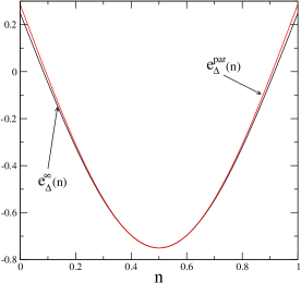
Figure 1: (Color online) Parametrization of $e_{\Delta}^{\mbox{\scriptsize par}}(n)$, given by Eqs. (V.1)-(92), compared to the exact ground state energy, $e_{\Delta}^{\infty}(n)$, for anisotropy $\Delta=-1/2$.

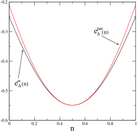
Figure 2: (Color online) Parametrization of $e_{\Delta}^{\mbox{\scriptsize par}}(n)$, given by Eqs. (V.1)-(92), compared to the exact ground state energy $e_{\Delta}^{\infty}(n)$ for anisotropy $\Delta=1/2$.

It is important to stress that the density of the interacting system is reproduced via the site-dependent magnetic fields $\{h_{i}^{s}\}$ of the non-interacting Kohn-Sham Hamiltonian (30). These effective fields depend on the difference of derivatives of the functionals at the anisotropy $\Delta$ and $\Delta=0$, i.e.,

$$h_{i}^{s}=h_{i}^{\mbox{\scriptsize ext}}+\frac{d}{dn}W_{\Delta}^{\mbox{\scriptsize LDA},\infty}(n)|_{n=n_{i}}.$$ (95)

In order to compare the effective magnetic fields produced by our parametrization $e_{\Delta}^{\mbox{\scriptsize par}}(n)$ with those obtained from the exact values for $e_{\Delta}^{\infty}(n)$, we show in Fig. 3 these fields, for $h_{i}^{\mbox{\scriptsize ext}}=0$, for two values of the anisotropies, in a system with constant density $n_{1}=\cdots=n_{L}=n$. In this case $h_{1}^{s},\ldots,h_{L}^{s}=h^{s}$. The exact results are obtained within computer accuracy from the numerical solutions of the Bethe ansatz equations given in the appendix, and the derivatives were obtained by using a cubic spline fitting of the numerical data. We see from this figure that for $0.4<n<0.6$ our parametrization (V.1)-(92) produces a rather good approximation for the local potentials in the Kohn-Sham Hamiltonian.

It is interesting to observe from Fig. 3 that the magnitude and even the sign of $h^{s}$ depend on the site density and on the value of the anisotropy $\Delta$. In Fig. 4 we show the effective magnetic field $h^{s}(n)$ obtained from the parametrization (90)-(V.1) for several values of the anisotropy $\Delta$. We see from this figure that while for $\Delta<0$ the magnetic field $h^{s}$ increases with the density $n$ of up spins, for $\Delta>0$ we have the opposite behavior. This is quite reasonable, since for $\Delta<0$ ($\Delta>0$) the net effect of the anisotropy is to increase (decrease) the energy as the density increases and the up spins are forced, in competition with the kinetic energy, to occupy nearest neighbor sites.

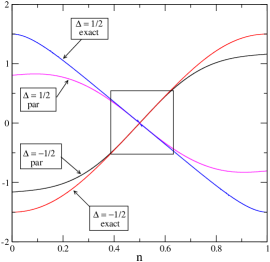
Figure 3: (Color online) Effective field $h^{s}=h_{1}^{s}=\cdots=h_{L}^{s}$ obtained from (95) with $h_{i}^{\mbox{\scriptsize ext}}=0$ as a function of the density $n=n_{1}=\cdots=n_{L}$ for two values of the anisotropies. The exact and approximate curves are obtained by using in (95) the parametrization (V.1)-(92) and the exact result, respectively.

Figure 4: (Color online) Effective field $h^{s}=h_{1}^{s}=\cdots=h_{L}^{s}$ obtained from (95) with $h_{i}^{\mbox{\scriptsize ext}}=0$ as a function of the density $n=n_{1}=\cdots=n_{L}$, for several values of the anisotropies. The curves were obtained by using the parametrization (V.1)-(92) in (V.1) and (95).

Next, we apply the LADA functionals (V.1) and (V.1), with (90)-(V.1), to several quantum chains whose ground state exhibits a spatially inhomogeneous distribution of up spins. Such inhomogeneities can be produced either by boundary conditions or by the presence of inhomogeneous external fields. We are going to consider example of both cases in the following subsections.

V.2 Open boundary conditions

As discussed in Sec. IV.3, except for the eigensector with total density $n=1/2$ of up spins ($L$ even), the eigenstates of the XXZ chain with open boundary conditions produce inhomogeneous density distributions even in the absence of external fields.

We have used the LADA approximation (V.1), with $e_{\Delta}^{\infty}(n)$ approximated by the parametrization for $e_{\Delta}^{\mbox{\scriptsize par}}(n)$ given by (V.1)-(94), to obtain the effective magnetic fields $\{h_{1}^{s},\ldots,h_{L}^{s}\}$ entering the Kohn-Sham Hamiltonian (30). Through a Jordan-Wigner transformationjordan-wigner this Hamiltonian is easily diagonalized for lattice sizes up to $L\approx 3000$. The density of up spins in the ground state is then calculated by diagonalizing (30) with (95). In order to compare our LADA predictions with exact results for small chains, we present in table 2 some of our spectral calculations at anisotropy $\Delta=-1/2$. The table displays the lowest energies $E_{\Delta}^{\mbox{\scriptsize open}}(L,\frac{1}{2}+\frac{\nu}{L})$ and the mass gaps $G_{L}^{\nu}$ (see (IV.3)) in the sectors with $N=\frac{L}{2}+\nu$ up spins ($\nu=0,1,2$) and lattice sizes $L=4$ to $24$. The exact results were obtained by a direct diagonalization of (III), and $\gamma=1$ was used in the LADA functional (V.1). We observe good agreement of the LADA predictions with the exact data, becoming better as the lattice size increases.

Table 2: Lowest eigenenergies in the sector with $N=\frac{L}{2}+\nu$ ($\nu=0,1$) up spins of the XXZ chain with open boundaries with $\Delta=-\frac{1}{2}$ and $L=4-24$. The 2nd and 4th (3rd and 5th) columns are the exact results (LADA results). The exact and LADA results for the gaps are shown in the 6th and 7th columns, respectively.

L	$E_{\Delta}^{\mbox{\scriptsize open}}(L,\frac{1}{2})$	$E^{\mbox{\scriptsize LADA},L,\mbox{\scriptsize open}}(L,\frac{1}{2})$	$E_{\Delta}^{\mbox{\scriptsize open}}(L,\frac{1}{2}+\frac{1}{L})$	$E^{\mbox{\scriptsize LADA},L,\mbox{\scriptsize open}}(L,\frac{1}{2}+\frac{1}{L})$	$LG_{L}^{1,\mbox{\scriptsize open}}$	$LG_{L}^{1,\mbox{\scriptsize LADA,open}}$
4	-0.678043	-0.644052	-0.437500	-0.387850	0.962172	2.624810
6	-0.699296	-0.676810	-0.581496	-0.549768	0.706798	0.762252
8	-0.710812	-0.694054	-0.640983	-0.618987	0.558637	0.600536
10	-0.718050	-0.704710	-0.671853	-0.655200	0.461971	0.495100
12	-0.723025	-0.711951	-0.690197	-0.676901	0.393828	0.420600
14	-0.726656	-0.717194	-0.702125	-0.691102	0.343425	0.365288
16	-0.729424	-0.721166	-0.710396	-0.700999	0.304446	0.321712
18	-0.731604	-0.724279	-0.713276	-0.708232	0.273446	0.288846
20	-0.733365	-0.726786	-0.720956	-0.713716	0.248198	0.261400
22	-0.734819	-0.728847	-0.724490	-0.717998	0.227235	0.238678
24	-0.736039	-0.730572	-0.727307	-0.721423	0.209568	0.219576

As discussed in Sec. IV, the mass-gap amplitudes of the finite-size corrections give the surface critical exponents $x_{\Delta}^{s,\nu}$ of the models (see Eq. (IV.3)). We verified, for arbitrary values of $\Delta$, that the LADA functional (V.1) with $\gamma=1$ and the parametrization (V.1) gives quite good predictions for the surface exponents. In tables 3 and 4 we show some of our estimates obtained for lattice sizes up to $L=512$. The finite-size estimates for the exponent $x_{\Delta}^{s,\nu}$ with $\nu=1$ and the ratio $x_{\Delta}^{s,2}/x_{\Delta}^{s,1}$ are presented in the last columns of these tables. Exact results in the thermodynamical limit $L\rightarrow\infty$ are shown in the last line of the tables. These results were derived from the Bethe ansatz equations (see appendix) and conformal invariance (see (69) and (24)).

Table 3: Lowest eigenenergies in the sector with $N=\frac{L}{2}+\nu$ ($\nu=0,1,2$) up spins of the XXZ chain with open boundaries and anisotropy $\Delta=-\frac{1}{2}$. The results were obtained by taking $\gamma=1$ and using the parametrization (V.1)-(92) in the LADA (V.1). In the 5th and 6th columns we show the finite-size estimates for the surface critical exponents $x_{\Delta}^{s,1}$ and the ratios $x_{\Delta}^{s,2}/x_{\Delta}^{s,1}$, respectively. The last line gives the expected exact results in the bulk limit ($L\rightarrow\infty$).

L	$a=E^{\mbox{\scriptsize open}}_{\Delta}(L,\frac{1}{2})/L$	$b=E^{\mbox{\scriptsize open}}_{\Delta}(L,\frac{1}{2}+\frac{1}{L})/L$	$c=E^{\mbox{\scriptsize open}}_{\Delta}(L,\frac{1}{2}+\frac{2}{L})/L$	$(b-c)L^{2}/\pi$	$\frac{c-a}{b-a}$
16	-0.721166	-0.700999	-0.641516	1.643310	3.949620
32	-0.735349	-0.730155	-0.714603	1.693019	3.994144
64	-0.742614	-0.741299	-0.737349	1.714280	4.003604
128	-0.746291	-0.745961	-0.744968	1.723679	4.003837
256	-0.748142	-0.748059	-0.747810	1.728007	4.002522
512	-0.749070	-0.749049	-0.748987	1.730070	4.001427
1024	-0.749535	-0.749529	-0.749513	1.731081	4.000765
1224	-0.749611	-0.749607	-0.749596	1.731302	4.000506
1424	-0.749665	-0.749663	-0.749655	1.731408	4.000439
${\infty\atop{({\rm exact})}}$	-0.75	-0.75	-0.75	1.732051	4

It is interesting, at this point, to discuss the effect of the parameter $\gamma$ in our LADA functional (V.1) (or (V.1)). Strictly speaking, $\gamma$ is a phenomenological parameter whose value was argued to be $\gamma\approx 1$ in Sec. V.1. The results presented in table 3 and 4 were obtained by setting $\gamma=1$. We have also calculated the quantities presented in table 3 and 4 for other values of $\gamma$. For $\Delta<0$ we got good results even from $\gamma=0$, where the nonlocal correction vanishes and the LADA functional reduces to the LDA. However for $\Delta>0$ (ferromagnetic regime) we get non-vanishing gaps for $\gamma=0$. This means that in this regime nonlocality is important for inhomogeneous density profiles and cannot be neglected. Good results are obtained for all values of $-1\leq\Delta<1$, as long as $0.98<\gamma<1.03$, which is consistent with our a priori expectation $\gamma\approx 1$.

Table 4: Same as table 3, but for anisotropy value $\Delta=+\frac{1}{2}$.

L	$a=E^{\mbox{\scriptsize open}}_{\Delta}(L,\frac{1}{2})/L$	$b=E^{\mbox{\scriptsize open}}_{\Delta}(L,\frac{1}{2}+\frac{1}{L})/L$	$c=E^{\mbox{\scriptsize open}}_{\Delta}(L,\frac{1}{2}+\frac{2}{L})/L$	$(b-c)L^{2}/\pi$	$\frac{c-a}{b-a}$
16	-0.532764	-0.528385	-0.513800	0.35684	4.330570
32	-0.540667	-0.539536	-0.535933	0.368617	4.186629
64	-0.544792	-0.544495	-0.543580	0.386752	4.084184
128	-0.546900	-0.546822	-0.546587	0.403868	4.029560
256	-0.547865	-0.547945	-0.547885	0.416341	4.008144
512	-0.548500	-0.548495	-0.548480	0.424043	4.001793
1024	-0.548769	-0.548768	-0.548764	0.428364	4.000165
1224	-0.548813	-0.548812	-0.548809	0.429098	4.000075
1424	-0.548845	-0.548844	-0.548842	0.429645	3.999887
${\infty\atop{({\rm exact})}}$	-0.549038	-0.549038	-0.549038	0.4330131	4

Let us now consider the density profiles $\{n_{1},\ldots,n_{L}\}$ of up spins on finite lattices. The Bethe ansatz for the finite chains, which would give the exact results for the density profiles, is impractical to solve. We have therefore considered lattice sizes we are able to diagonalize numerically. In Fig 5 we show, for $L=24$ sites, an example of the exact and LADA prediction for the density profile $\{n_{1},\ldots,n_{24}\}$ of the XXZ chain with open boundaries. The densities shown in the figure are obtained from the lowest eigenenergy in the sector with $n=11$ up spins and anisotropy $\Delta=-\frac{1}{2}$. We see from this figure that although the LADA amplitudes are smaller than the exact ones, they exhibit the same spacial oscillations. These spacial oscillations should decrease in amplitude as the lattice size increases. In Fig 6 we show the density profiles predicted by our LADA functional (V.1) with the parametrization function (V.1) and $\gamma=1$, for several lattice sizes. The density profiles correspond to the lowest eigenstate in the sector with $N=\frac{L}{2}+1$ spins at anisotropy $\Delta=-\frac{1}{2}$. We have scaled the vertical and horizontal axis of Fig. 6, in order to display simultaneously the density profiles of distinct lattice sizes. This figure shows that the amplitude of the oscillations decreases as $O(L^{-1})$, as the lattice size increases.

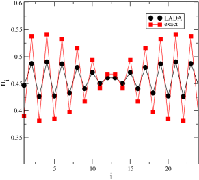
Figure 5: (Color online) Exact and LADA predictions for the density profile $n(i)$ of up spins for the XXZ quantum chain with open boundaries and $\Delta=-\frac{1}{2}$. The profiles correspond to the lowest eigenenergy in the sector with $N=11$ up spins of the quantum chain with $L=24$ sites.

V.3 Periodic boundary condition with inhomogeneous external magnetic fields

A physically distinct way to produce inhomogeneous density profiles $\{n_{1},\ldots,n_{L}\}$ of up spins is the presence of external magnetic fields $\{h_{1}^{\mbox{\scriptsize ext}},\ldots,h_{L}^{\mbox{\scriptsize ext}}\}$. In this case, as in the case of open boundaries, we have to solve the Kohn-Sham Hamiltonian (30)-(31) selfconsistently.

In order to compare our results to the exact ones, we show in Fig. 7 the density profile obtained by using the LADA functional (V.1) with $e_{\Delta}^{\infty}(n)$ replaced by $e_{\Delta}^{\mbox{\scriptsize par}}(n)$ given by (V.1). The density profiles of Fig. 7 correspond to the lowest energy in the sector with $N=12$ up spins of the periodic XXZ chain with $L=24$ sites and anisotropy $\Delta=-\frac{1}{2}$. The external local magnetic fields are chosen to be $h_{i}^{\mbox{\scriptsize ext}}=\delta_{i,11}$. Similar to Fig. 5, the LADA densities have smaller amplitudes than the exact ones, but exhibit the same spacial oscillations.

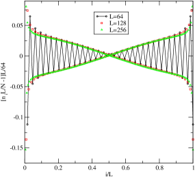
Figure 6: (Color online) LADA predictions for the density profiles $n(i)$. The profiles correspond to the lowest eigenenergy in the sector with $N=\frac{L}{2}-1$ up spins of the XXZ quantum chain with $L$ sites ($L=64,128,256$), open boundaries and anisotropy $\Delta=-\frac{1}{2}$.

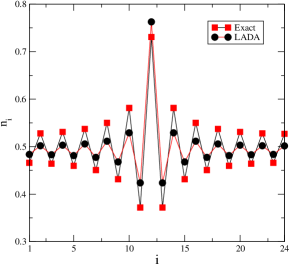
Figure 7: (Color online) Exact and LADA results for the density profiles corresponding to the ground state of the XXZ quantum chain with periodic boundaries and inhomogeneous magnetic fields. The profiles correspond to the quantum chain with $L=24$ sites, $N=12$ up spins, anisotropy $\Delta=-\frac{1}{2}$, and inhomogeneous magnetic fields $h_{i}^{\mbox{\scriptsize ext}}=\delta_{i,11}$ ($i=1,\ldots,24$).

One of the main purposes of this paper is to present density functionals that are able to predict the critical exponents of critical chains from finite-size corrections to the mass gap. In order to test the LADA functional (V.1) with (V.1) we study the periodic XXZ chain with a single impurity, represented by the external magnetic field $h_{i}^{\mbox{\scriptsize ext}}=\delta_{i,1}$ ($i=1,\ldots,L$). The presence of such impurity breaks spin reversal symmetry, but we expect, as $L\rightarrow\infty$, the leading behavior for the average mass gap

$$\bar{G}_{L}^{\nu\mbox{\scriptsize per}}=\frac{1}{2}[E_{\Delta}^{\mbox{\scriptsize per}}(L,\frac{1}{2}+\frac{\nu}{L})+E_{\Delta}^{\mbox{\scriptsize per}}(L,\frac{1}{2}-\frac{\nu}{L})$$

$$-2E_{\Delta}^{\mbox{\scriptsize per}}(L,\frac{1}{2})]$$ (96)

$$=\frac{\pi}{L}v_{\Delta}x_{\Delta}^{s,\nu}+o(\frac{1}{L}),$$ (97)

where $v_{\Delta}$ is the sound velocity (45) and $x_{\Delta}^{s,\nu}$ the surface exponents ($\nu=1,2,\ldots$). In Eq. (V.3) $E_{\Delta}^{\mbox{per}}(L,n)$ is the lowest energy in the sector with $N=nL$ up spins of the periodic chain with anisotropy $\Delta$ and $L$ sites. In table 5 we present the finite-size estimates for the critical exponents $x_{\Delta}^{s,\nu}$ of the quantum chain with $\Delta=-\frac{1}{2}$ and lattice sizes up to $L=1024$. In the last line we show the expected exact results in the bulk limit $L\rightarrow\infty$. Clearly, the LADA functional (V.1) with parametrization (V.1) gives reliable results for the critical exponents.

Table 5: LADA predictions for the ground state energy and finite-size estimates of the average mass gaps (V.3) for the XXZ chain with periodic boundaries and inhomogeneous magnetic fields. The results were derived for the anisotropy value $\Delta=-\frac{1}{2}$ and inhomogeneous fields $h_{i}^{\mbox{\scriptsize ext}}=\delta_{i,L/2}$ ($i=1,\ldots,L$). In the last line it is shown the expected results in the bulk limit ($L\rightarrow\infty$).

L	$E_{\Delta}^{\mbox{\scriptsize per}}(L,\frac{1}{2})$	$L{\bar{G}}_{L}^{1,\mbox{\scriptsize per}}\pi$	$L{\bar{G}}_{L}^{2,\mbox{\scriptsize per}}\pi$	${\bar{G}}_{L}^{2,\mbox{\scriptsize per}}/{\bar{G}}_{L}^{1,\mbox{\scriptsize per}}$
8	-0.736502	1.646049	6.211188	3.773392
16	-0.738800	1.685301	6.657321	3.950226
32	-0.743287	1.707394	6.816070	3.992090
64	-0.746363	1.719601	6.879476	4.000623
128	-0.748111	1.725632	6.905708	4.001843
256	-0.749038	1.728826	6.917514	4.001278
512	-0.749515	1.730444	6.923041	4.000730
1024	-0.749756	1.731253	6.925686	4.000389
${\infty\atop{({\rm exact})}}$	-0.75	1.732051	6.928204	4

VI Conclusions

In this work we explored the possibility to obtain reliable results for critical exponents, conformal anomalies, and related quantities of quantum chains from density functionals. Due to conformal invariance, the critical exponents are obtained from the $O(1/L)$ finite-size corrections of the mass gaps of the quantum chains in finite geometries. These finite-size corrections can be obtained approximately from DFT. In order to test our general approach, we performed an extensive study of various LDA and beyond LDA functionals for the exactly integrable XXZ quantum chain in the critical regime $-1\leq\Delta<1$.

Our functionals are obtained from a formal gradient expansion of the unknown exact functional around homogeneous distributions of the infinite system. The first term of this expansion gives LDA functionals, appropriate for cases where the density distribution in the chain is weakly inhomogeneous, or fully homogeneous. The latter is the case when the quantum chain is defined on translationally invariant lattices, with periodic and twisted boundary conditions (see Eqs. (39) and (56)). As we saw in Sec. IV, even a simple LDA can give exact critical exponents, but a direct evaluation of the conformal anomaly from these functionals gives wrong results because the sound velocity, a nonuniversal constant, has distinct values for the interacting Hamiltonian and the non-interacting auxiliary Kohn-Sham Hamiltonian. A correct LDA prediction of the conformal anomaly $c=1$, for any value of the anisotropy $\Delta$, can be obtained only if we rescale the interacting and non interacting quantum chain by its appropriate sound velocity. This is certainly a problem for general quantum chains whose sound velocity is unknown. A possible solution is the use of a size-dependent LDA, which embodies nonlocal corrections in a simple way.

In the case of open boundaries, only eigenstates belonging to the sector with $N=L/2$ up spins have a homogeneous distribution on the quantum chain with finite size $L$. In this case, the surface energy of the quantum chain is predicted incorrectly, for the same reason discussed above for the sound velocity and conformal anomaly. However, as we showed in Sec. IV (see Eq. (77)), application to a properly rescaled Hamiltonian gives correct results, as does use of a finite-size LDA.

If the density distribution is inhomogeneous, our results indicate that we must also consider at least the second term of the expansion (15)-(II.2) of the exact functional. The LADA functional derived from this term for quantum chains with periodic and open boundary conditions is given by (V.1) and (V.1), respectively. These functionals can be used, in principle, for a general quantum chain, by replacing $e_{\Delta}^{\infty}(n)$ by an approximate expression $e^{\mbox{\scriptsize hom}}(n)$ for the ground state energy per site of the infinite system with density $n$. In this general case, the quality of the resulting prediction of critical exponents, via evaluation of gaps, depends on the quality of approximations for $e^{\mbox{\scriptsize hom}}(n)$. For an exactly integrable chain, like the XXZ quantum chain, the energy per site $e_{\Delta}^{\infty}(n)$ can be obtained exactly, e.g., by solving the integral equation derived from the Bethe ansatz (see (98)-(A) in the appendix). Instead of using such numerical results for $e_{\Delta}^{\infty}(n)$ we proposed, in Sec. V, an approximate parametrization $e_{\Delta}^{\mbox{\scriptsize par}}(n)$, Eq. (V.1), containing all essential ingredients to furnish good estimates for the critical exponents of the XXZ quantum chain in the presence of small inhomogeneities.

Both the finite-size LDA and the LADA functional are nonlocal density functionals, the former depending on the local density and the size of the system, the latter depending on the local and the average density. Unlike the usual (infinite-size) LDA, these functionals also depend, in a known way, on the boundary conditions (open, periodic, or twisted). As a consequence of this nonlocality, the finite-size LDA and the LADA functional each cure certain defects of the LDA. For finite homogeneous chains, the LDA reproduces the correct critical exponents, but predicts a wrong conformal anomaly, whereas the finite-size LDA correctly reproduces both. For inhomogeneous chains, the LADA functional yields better energies and gaps than the LDA. For finite homogeneous chains, the LADA functional reduces to the LDA. The combination of both improvements, i.e., the construction of a finite-size LADA is a promissing project for the future.

Another interesting question concerns possible extensions of the LADA functional (V.1)-(V.1) to other quantum chains in the $c=1$ universality class. Consider a general homogeneous model on this universality class. The introduction of a homogeneous magnetic field (or chemical potential) $h(n)$ that couples to the density operator $\hat{n}_{i}$ will produce a ground state with energy per site $e(n)$ and homogeneous density $n$. In order to fix the density $n$, this magnetic field should satisfy $h(n)=\frac{de(n)}{dn}$. The critical exponents with such external field are given by Eq. (22) with $x=x(n)$, depending on the particular density fixed by $h(n)$. Besides $x(n)$ and $h(n)$, the quantum chain is also characterized by the non-universal sound velocity $v(n)$ that fixes the scale of the momentum-energy dispersion relation. The results coming from conformal invariance for this class of models give us a generalization of Eq. (48) for arbitrary densities, i.e., $\frac{d^{2}e(n)}{dn^{2}}=4\pi v(n)x(n)$.

In order to obtain the density distribution $\{n_{i}\}$ when inhomogeneous external fields or boundaries are added to the homogeneous system we may proceed in two ways. If the local density never exceeds unity, the XY model (30) can be used as the auxiliary non-interacting (Kohn-Sham) system. If this is not the case, the only remaining possibility is the direct use of the approximate functional for $F_{I}$ in the Euler equation (6). The first case is preferable, since the LDA functional is not exact and the auxiliary non-interacting chain will give a more precise evaluation of the kinetic energy contained in $F_{s}$. In both approaches, the necessary quantities for the evaluation of the density are $h(n)$ and $4\pi v(n)x(n)$.

To conclude, let us briefly discuss some possible future developments of the present work. The functional we produce gives us mass gaps of finite chains that produce reasonable, in some cases even exact, estimates for the critical exponents. A second possibility to obtain the critical exponents is from the power-law decay of the Friedel density oscillations due to the presence of impurities on the quantum chain.friedel Tests with the LADA functionals (V.1) or (V.1) for the XXZ chain with open and periodic boundary condition indicate poor results in this case. This means that the correct decay of the Friedel density oscillations can only be obtained by considering higher order terms in the expansion (15)-(II.2). This is certainly an interesting point for the future.

*

Appendix A Integral equations derived from the Bethe ansatz solution of the XXZ quantum chain

The ground state energy per site, $e_{\Delta}^{\infty}(n)$, of the XXZ chain, in the bulk limit, can be obtained from the Bethe ansatz solution of the model (see e.g. Ref. hamer, ).

For $-1\leq\Delta<1$, by setting $\Delta=-\cos\gamma$

$$e_{\Delta}^{\infty}(n)=\frac{\cos\gamma}{2}-2\int_{-\Lambda}^{\Lambda}\frac{\sin^{2}\gamma}{\cosh\eta-\cos\gamma}R(\eta)d\eta,$$ (98)

where the parameter $\Lambda$ fix the density $n$ through

$$\int_{-\Lambda}^{\Lambda}R(\eta)d\eta=n.$$ (99)

The function $R(\eta)$ is obtained by solving the integral equation

$$R(\eta)=\frac{1}{2\pi}\left[\frac{\sin\gamma}{\cosh\eta-\cos\gamma}\right.$$

$$\left.-\int_{-\Lambda}^{\Lambda}\frac{\sin 2\gamma}{\cosh(\eta-\eta^{\prime})-\cos 2\gamma}R(\eta^{\prime})d\eta^{\prime}\right].$$ (100)