Loschmidt echoes in two-body random matrix ensembles

Abstract

Fidelity decay is studied for quantum many-body systems with a dominant independent particle Hamiltonian resulting e.g. from a mean field theory with a weak two-body interaction. The diagonal terms of the interaction are included in the unperturbed Hamiltonian, while the off-diagonal terms constitute the perturbation that distorts the echo. We give the linear response solution for this problem in a random matrix framework. While the ensemble average shows no surprising behavior, we find that the typical ensemble member as represented by the median displays a very slow fidelity decay known as “freeze”. Numerical calculations confirm this result and show that the ground state even on average displays the freeze. This may contribute to explanation of the “unreasonable” success of mean field theories.

I Introduction

Wigner wigner1 proposed the use of random matrix theory, in particular of the classical ensembles cartan ; brody to explain statistical properties of nuclear spectra. Balian balian showed that this amounts to using a minimum information approach, where symmetry is the only characteristics taken into account. An essential element for the widespread success guhr resides in the ergodicity of the results obtained for classical ensembles. Yet it was soon noticed frenchPL33B ; bohigasPL34B that the essential two-body character of the underlying interaction requires embedded ensembles, in particular the two-body random matrix ensemble (TBRE). While the original work carried the full weight of a three dimensional few nucleon system, soon abstract models with structureless fermions were introduced french2 to understand more easily embedded ensembles in general and the TBRE in particular. Two problems beset these studies: one is the apparent non-ergodicity of these ensembles, the other is the difficulty to obtain any analytical results (see benet for a review). After individual unfolding of each spectrum brody ; bohigasPL34B spectral statistics of the classical ensembles are recovered and this marginated the interest in embedded ensembles for some time. Interest was rekindled recently mainly by studies of interesting properties at the edge of the spectra concerning ground states bertsch1 ; papenbrockweiden ; frank . The question whether the ensemble is actually ergodic or not remains open benet , but French french3 ; benet has shown that it is somewhat academic, as even the spectral density has fluctuations of the order $1/\log N$ where $N$ is the dimension of the Hilbert space. This makes individual unfolding essential for any statistical analysis of spectra. The reason why individual unfolding does lead to the right answers is not understood to this day. The renewed interest in the TBRE has spread to various fields including applications benet ; zelevinsky ; floresseligman and extensions to bosons kota ; benet .

Fidelity analysis for the stability of quantum systems under perturbation, first proposed by Peres peresPRA30 , has become very fashionable since the advent of quantum information where it provides a standard criterion nielsenbook of stability; for a recent review see fidelityreview . It seems reasonable to check how a small residual two-body interaction affects the stability of the solution of an independent particle Hamiltonian. The diagonal part of this interaction does not affect the eigenstates and is usually included in the independent particle term, known as the mean field approximation.

We focus on the validity of the mean field approximation, given by the stability of the time-dependent solution of the mean field Hamiltonian which is measured by fidelity. This is also the main physical motivation behind defining the random matrix model in the present paper.

Fidelity has been calculated by the method of stationary phase applied to time-dependent propagator for semi-classical considerations jalabert ; cucchietti ; lewenkopf ; vanicek and by super-symmetric techniques stoeckmannNJP ; stoeckmannPRE73 for a random matrix model presented in gorinNJP6 . In both contexts most of the relevant results can be obtained by perturbative or linear response techniques, which actually do not require either model as a basis P02 ; PZ02 ; Progress ; gorinNJP6 ; fidelityreview ; G-prl . Even in the regime where fidelity is not anymore close to one, a simple exponentiation of the leading term yields excellent results far beyond this regime Progress ; fidelityreview . Crossovers between semiclassical and perturbative considerations (the latter also known as Fermi Golden rule regime) have been discussed in jacquodPRE ; cerruti . A drastic reduction of fidelity decay termed “fidelity freeze” occurs when the perturbation is strictly off diagonal (or more generally, when its time average is zero) freezeint ; freezech ; G-prl . Such a situation can occur when perturbation breaks the antiunitary symmetry (like time-reversal) of the unperturbed Hamiltonian in an optimal way G-prl , which can perhaps be experimentally realized by some magnetic interactions.

In case of high level fidelity freeze the dynamics is stable for a very long time. The question is whether we can see this effect in the situation under consideration. On the one hand our system looks promising, due to the inclusion of the diagonal part of the interaction in the “unperturbed” independent particle Hamiltonian. On the other hand the occurrence of the freeze in random matrix models depends heavily on level repulsion implicit in a GOE or a GUE for the unperturbed system. Clearly the independent particle model does not have this repulsion and indeed we can expect results similar to those of a random spectrum where absence of a diagonal perturbation to lowest order only suppresses the quadratic decay fidelityreview .

Our analysis will show that the ensemble average does not display fidelity freeze. The typical ensemble member however does show this freeze. This is confirmed when we consider the median of fidelity rather than its average. This fact is important by itself as it shows that quantum evolution of the full problem will follow that of the independent particle problem or mean field approximation for a very long time for most systems. It also is important because it shows that RMT models can describe physical situations qualitatively, even when the average behavior is completely off. The last point can also be reformulated as a necessity to look at the right quantities i.e. quantities whose distributions have no long tails. If we had replaced fidelity by distortion as introduced in an elastic problem weaver , then the average and median would coincide. This results because distortion is defined as the logarithm of one minus fidelity gorin-weaver . Indeed in other contexts taking averages of the logarithm is a common remedy to eliminate exaggerated effects of tails in distributions leyvraz-privat . Furthermore we will see that for the ground state and the first excited state of the independent particle model the freeze will occur even on average.

After introducing basics about fidelity and the Hamiltonian we will see that under specific assumptions for the independent particle spectrum we can obtain ensemble averaged fidelity decay of a TBRE in the linear response regime. The result essentially yields the linear decay. Yet a numerical inspection of individual Hamiltonians in the ensemble shows the existence of fidelity freeze. A more careful numerical analysis shows that the median fidelity for the ensemble indeed displays the freeze. Thus we can consider it as typical. This result is quantitatively reconfirmed by showing that the ensemble averaged logarithm of one minus fidelity also displays the freeze. We relate this behavior directly to the existence of a gap in the nearest neighbor spacing distribution of the independent particle spectrum. Furthermore we find that the fidelity decay of the ground and first excited state of the independent particle Hamiltonian display the freeze even on average. Next we numerically check different options for the single particle spectrum to obtain a better feeling of the non-ergodicity, which plays a central role in this context. Finally we give some conclusions.

II Fidelity amplitude

The fidelity amplitude measures the overlap between two quantum states $\psi_{0}(t^{\prime})$ and $\psi(t^{\prime})$ evolving from the same initial state $\psi(0)$ but propagated with slightly different Hamiltonians $H_{0}$ and $H=H_{0}+\lambda V$ respectively

$$f(t^{\prime})=\langle\psi_{0}(t^{\prime})|\psi(t^{\prime})\rangle=\langle\psi(0)|\mathrm{e}^{\frac{\mathrm{i}}{\hbar}t^{\prime}H_{0}}\mathrm{e}^{-\frac{\mathrm{i}}{\hbar}t^{\prime}H}|\psi(0)\rangle.$$ (1)

For small perturbation strength $\lambda$ it is convenient to use a linear response or Born expansion P02 ; PZ02 ; fidelityreview . We shall follow the notation established in gorinNJP6 as it is well adapted to RMT. In the interaction picture the wave function reads as $x(t^{\prime})=\mathrm{e}^{\frac{\mathrm{i}}{\hbar}H_{0}t^{\prime}}\psi(t^{\prime})$. Time $t^{\prime}$ can be replaced by dimensionless time $t$ measured in units of the Heisenberg time $t_{H}=2\pi\hbar/d$ where $d$ denotes the average level spacing in the spectra of $H_{0}$ which can and will be set to one. Therefore, the time will always be given in units of $t_{H}$. Time evolution of a state $x(t)$ up to the second order $x^{(2)}(t)=X(t)x(0)$ in perturbation strength $\lambda$ can be expressed as

$$X(t) = 1-2\pi\lambda\mathrm{i}\int_{0}^{t}\mathrm{d}t_{1}V_{I}(t_{1})$$ (2)

$$- (2\pi\lambda)^{2}\int_{0}^{t}\mathrm{d}t_{1}\int_{0}^{t_{1}}\mathrm{d}t_{2}V_{I}(t_{1})V_{I}(t_{2})$$

where $V_{I}(t)$ is the abbreviation for the perturbation in the interaction picture $V_{I}(t)=\mathrm{e}^{2\pi\mathrm{i}H_{0}}V\mathrm{e}^{-2\pi\mathrm{i}H_{0}}$. Please note that the expansion in (2) is valid even for times much longer than the Heisenberg time ($t\gg 1$), if only the perturbation strength is small enough.

The fidelity amplitude for an initial state ${|x(0)\rangle}=\sum_{j}x_{\alpha}|\alpha\rangle$ written as a superposition of independent particle states, i.e. state eigenstates of the unperturbed Hamiltonian ${|\alpha\rangle}$, then reads

$$f(t)=\langle x(0)|X(t)|x(0)\rangle=\sum_{\alpha,\beta=0}^{\mathcal{N}}X_{\alpha\beta}x_{\alpha}^{*}x_{\beta}.$$ (3)

Later we consider ensemble averages. Then the linear term in (2) vanishes and the matrix element $X_{\alpha\beta}$ is reduced to contributions from the quadratic term only.

III The Hamiltonian

Although a simple RMT of full Gaussian matrices often yields impressively accurate results, it, strictly speaking, only applies to dynamical systems where all levels are coupled by the interaction. More realistic physical systems such as nuclear or atomic shell models or quantum dots do not possess that property. The interaction involves two particles only. In the framework of RMT it should be described by Two-Body Random Ensembles (TBRE) frenchPL33B ; bohigasPL34B ; brody ; zelevinsky ; benet . We consider a system of $M$ “spinless” Fermi particles in $N$ orbitals in the presence of fermion-fermion interaction. We shall use second quantization notation with fermion creation and annihilation operators $c_{i}^{\dagger}$ and $c_{i}$ fulfilling the usual anticommutation relations and creating or annihilating a fermion in the $i$th eigenstate of the single particle Hamiltonian defined by the mean field. The $M$ particle eigenstate ${|\alpha\rangle}=(c_{0}^{\dagger})^{\alpha_{0}}\cdots(c_{N-1}^{\dagger})^{\alpha_{N-1}}{|0\rangle}$ (where exactly $M$ binary digits $\alpha_{i}$ of integer $\alpha$ are equal to $1$) of the independent particle Hamiltonian is then a product of $M$ creation operators with distinct indices applied to a vacuum state. The Hamiltonian is written in the usual manner as

$$H=\sum_{i}e_{i}c_{i}^{\dagger}c_{i}+\lambda\sum_{i<j,k<l}V_{ijkl}c_{i}^{\dagger}c_{j}^{\dagger}c_{l}c_{k},$$ (4)

where all Latin indices are running from $0$ to $N-1$, and where the $e_{i}$ are ordered single-particle energies, $V_{ijkl}$ are properly antisymmetrized two-body matrix elements and $\lambda$ is the perturbation strength. The unperturbed Hamiltonian $H_{0}$ will correspond to the Mean Field Approximation and will hence be chosen as the one-body terms $\sum_{i}e_{i}c_{i}^{\dagger}c_{i}$ plus the diagonal part of the interaction $\lambda\sum_{i<j}V_{ijij}c_{i}^{\dagger}c_{j}^{\dagger}c_{j}c_{i}$. A natural question is how the remaining part of $V$, which we shall consider as perturbation, affects the dynamics.

The inclusion of the diagonal part of the interaction in the unperturbed system is crucial to our argument. On one hand it does not affect the eigenfunctions of the one-particle term and thus it seems of little importance. Yet in the calculation of fidelity the dephasing it produces, becomes the dominant term. On the other hand, if included in the unperturbed part it will only enter the result to the fourth order in ${\lambda}$ because the spectral two-point function will only enter to order $\lambda^{2}$ and it, in turn, will only be affected to order $\lambda^{2}$ by the diagonal terms.

So far we have not put any constraints on the spectral properties of $H_{0}$ nor on the perturbation $V$. The latter consists of independent two-body matrix elements, where the weight coefficients $V_{ijkl}$ are chosen as independent random Gaussian complex numbers with vanishing mean and $\langle V_{ijkl}V_{mnop}\rangle_{V}=v^{-2}\delta_{ij,op}\delta_{kl,mn}$, where the variance $v^{-2}$ is set to normalize the perturbation as $\langle{\rm tr}[V^{2}]\rangle=\mathcal{N}$ where $\mathcal{N}={N\choose M}$ is the dimension of full Hilbert space. The unperturbed dynamics is given by $N$ single-particle levels $e_{j}$. We shall often choose them as the eigenvalues of the $N\times N$ Hermitian matrix chosen from the GUE, but we shall mention other options and their consequences. Similar models have recently been widely studied e.g. in nuclear physics flambaum and for studying chaotic quantum dots alhassid .

Two-body operators $c_{i}^{\dagger}c_{j}^{\dagger}c_{l}c_{k}$ can be split into three groups by inspecting indices $i,j,k,l$: diagonal terms with two pairs of equal indices, three-orbital terms with one pair of equal indices, and four-orbital terms without pairs of equal indices. The non-zero matrix elements $V_{\alpha\beta}$ in the full Hilbert space therefore couple many-particle states which differ by at most two single-particle states and these states are the only intermediate states in a two-fold transition described by $V_{I}(t_{1})V_{I}(t_{2})$ in (2). After averaging over an ensemble of two-body interactions all products of independent $V_{ijkl}$ vanish and our interest is narrowed to transitions with the same initial and final state described by averaged matrix elements $\langle[V(t_{1})V(t_{2})]_{\alpha\beta}\rangle_{V}=\delta_{\alpha\beta}C_{\alpha}(t_{1}-t_{2})$ which only depend on the time difference and are denoted by the correlation function $C_{\alpha}(\tau)$. Using $H_{0}\equiv{\rm diag}(h_{\alpha})$, which $h_{\alpha}$ is either single particle Hamiltonian $h_{\alpha}={\langle\alpha|}\sum_{i}{\hat{n}_{i}}e_{i}{|\alpha\rangle}$, ${\hat{n}_{i}}=c_{i}^{\dagger}c_{i}$, or the mean field Hamiltonian $h_{\alpha}={\langle\alpha|}\sum_{i}{\hat{n}_{i}}e_{i}+\lambda\sum_{i<j}V_{ijij}{\hat{n}_{i}}{\hat{n}_{j}}{|\alpha\rangle}$, the correlation function can be written as

$$C_{\alpha}(\tau) = \sum_{\gamma}\langle\mathrm{e}^{2\pi\mathrm{i}h_{\alpha}}V_{\alpha\gamma}\mathrm{e}^{-2\pi\mathrm{i}h_{\gamma}}V_{\gamma\alpha}\rangle_{V}$$ (5)

$$= \sum_{\gamma}\langle\mathrm{e}^{-2\pi\mathrm{i}(h_{\gamma}-h_{\alpha})}\rangle_{V}\langle V_{\alpha\gamma}V_{\gamma\alpha}\rangle_{V}.$$

The first average is nontrivial in the mean field case where the energy differences $h_{\gamma}-h_{\alpha}$ contain also diagonal two-body terms (mean field). The correction to $\mathrm{e}^{-2\pi\mathrm{i}\sum_{j}({\langle\gamma|}{\hat{n}_{j}}{|\gamma\rangle}-{\langle\alpha|}{\hat{n}_{j}}{|\alpha\rangle})e_{j}}$ due to mean field is of order $\mathcal{O}(\lambda^{2})$. As mentioned above, since the correlation function will enter the linear response formula for fidelity gorinNJP6 with a prefactor $\lambda^{2}$, the overall correction to the fidelity amplitude is $\mathcal{O}(\lambda^{4})$ and will be neglected. We split the $C_{\alpha}(\tau)$ into three groups according to the classification of two-body transitions

$$C_{\alpha}(\tau) = \langle\alpha|v^{-2}\sum_{kl}c_{k}^{\dagger}c_{l}^{\dagger}c_{l}c_{k}c_{k}^{\dagger}c_{l}^{\dagger}c_{l}c_{k}$$

$$+ v^{-2}\sum_{i\neq k,j}c_{k}^{\dagger}c_{j}^{\dagger}c_{j}c_{i}c_{i}^{\dagger}c_{j}^{\dagger}c_{j}c_{k}\mathrm{e}^{-2\pi\mathrm{i}(e_{i}-e_{k})\tau}$$

$$+ v^{-2}\!\!\!\sum_{i<j\neq k<l}\!\!\!c_{k}^{\dagger}c_{l}^{\dagger}c_{j}c_{i}c_{i}^{\dagger}c_{j}^{\dagger}c_{l}c_{k}\mathrm{e}^{-2\pi\mathrm{i}(e_{i}+e_{j}-e_{k}-e_{l})\tau}|\alpha\rangle.$$

The abbreviation in the last sum means that indices $i,j,k,l$ are all different. The first term of (III) is actually only present if we would be interested in considering the full two-body term as perturbation and thus consider the corresponding dephasing . Partially summing the expression yields

$$C_{\alpha}(\tau) = v^{-2}{M\choose 2}+v^{-2}(M-1)\sum_{ik}n_{k}{\bar{n}_{i}}\mathrm{e}^{-2\pi\mathrm{i}(e_{i}-e_{k})\tau}$$ (7)

$$+ v^{-2}\frac{1}{4}\sum_{ijkl}{\bar{n}_{i}}{\bar{n}_{j}}n_{k}n_{l}\mathrm{e}^{-2\pi\mathrm{i}(e_{i}+e_{j}-e_{k}-e_{l})\tau}$$

Here $n_{i}\!=\!\langle\alpha|c_{i}^{\dagger}c_{i}|\alpha\rangle$ indicates the Fermion occupation number and we use the convention ${\bar{n}_{i}}\!=\!1\!-\!n_{i}$. The relation between the fidelity amplitude and the correlation function after averaging over the interaction reads

$$\langle f(t)\rangle_{V}=\sum_{\alpha}|x_{\alpha}|^{2}\Big{[}1-4\pi^{2}\lambda^{2}\int_{0}^{t}\!\mathrm{d}t_{1}\int_{0}^{t_{1}}\!\mathrm{d}t_{2}C_{\alpha}(t_{1}-t_{2})\Big{]}.$$ (8)

If the spectrum of $H_{0}$ is known, this allows us to determine the fidelity amplitude by integrating the correlation function in (III) twice for each eigenstate $\alpha$ and evaluate the sum in (8). Actually we are more interested in ensemble behavior which we shall study in the next two subsections.

IV Ensemble averaged fidelity amplitude

Relation (8) can be simplified if we average over initial states or select a random initial state by choosing Gaussian random coefficients $x_{\alpha}$ normalized by the requirement $\langle|x_{\alpha}|^{2}\rangle_{0}=1/\mathcal{N}$. The correlation function can be averaged as $C(\tau)=\frac{1}{\mathcal{N}}\sum_{\alpha}\langle C_{\alpha}(\tau)\rangle_{0}$ which implies averaging over all distributions of $M$ particles on $N$ orbitals. We find

$$C(\tau) = \frac{v^{-2}}{\mathcal{N}}(M-1){N-2\choose M-1}\sum_{m\neq n}\langle\mathrm{e}^{-2\pi\mathrm{i}(e_{m}-e_{n})\tau}\rangle_{0}+$$ (9)

$$+ \frac{v^{-2}}{\mathcal{N}}{N-4\choose M-2}\!\!\sum_{m\neq n\neq p\neq q}\!\!\!\!\!\!\!\langle\mathrm{e}^{-2\pi\mathrm{i}(e_{m}+e_{n}-e_{p}-e_{q})\tau}\rangle_{0}.$$

A closer inspection of first term in (9) shows that it is connected with the probability distribution of pairs of energies of two arbitrary orbitals which is given by Dyson’s two-point correlation function $R_{2}$ following the definition in mehtabook . The average can then be obtained by integration. A similar argument connects the second average with the four-point correlation function $R_{4}$. Finally, using the normalization factor $v^{2}={M\choose 2}\big{(}2(N-M)+{N-M\choose 2}\big{)}$ we rewrite the correlation function in compact form (using $\eta=\frac{N-M-1}{4}$)

$$C(t) = \frac{1}{1+\eta}\mathcal{F}[R_{2}]\left(\frac{2\pi\sqrt{2}t}{d}\right)+$$ (10)

$$+ \frac{1}{1+\eta^{-1}}\mathcal{F}[R_{4}]\left(\frac{2\pi\sqrt{2}t}{d}\right).$$

The functions $\mathcal{F}[R_{n}](t)$ are obtained by Fourier transformation of the correlation functions $R_{n}$ (see Appendix for precise definitions). In the case of GUE single-particle spectra, the functions $\mathcal{F}[R_{n}](t)$ can be calculated analytically and are given as products of finite polynomials in $t$ and Gaussians (see Appendix). They are normalized such that $\mathcal{F}[R_{2,4}](0)=1$.

The simulations have been performed both including and excluding the diagonal terms of the two-body interaction and coincide with the theoretical prediction in (10) (or the corresponding full calculation) if the random states are chosen from the whole energy spectrum or from its center. The ensemble and state averaged fidelity amplitude can now be obtained by integrating the averaged correlation function in (10) twice

$$\langle f(t)\rangle=1-4\pi^{2}\lambda^{2}\int_{0}^{t}\mathrm{d}t_{1}\int_{0}^{t_{1}}\mathrm{d}t_{2}C(t_{1}-t_{2}).$$ (11)

In the residual case where the perturbation $V$ has no diagonal terms (i.e. in the case of mean field unperturbed Hamiltonian) the correlation function has no constant term. The correlation integral can then be approximated by a linear function for fairly long times as long as the linear response formalism is justified. The simulation (Fig. 1) is done with random initial states from the center of the spectra and is in agreement with the full-spectra prediction. The residual case thus coincides qualitatively with the result of a general residual perturbation of a Hamiltonian with a random spectrum G-prl ; fidelityreview also known as POE dittes . Fidelity freeze is not found and we could easily conclude that this exercise is rather disappointing. Yet, considering the known non-ergodicity of the TBRE, it seems worthwhile to check whether the average behavior reflects the typical behavior.

Figure 1: Fidelity amplitude decay for $6$ particles in $12$ orbitals averaged over $2\cdot 10^{5}$ realizations of $V$, $H_{0}$ and initial states, with the perturbation strength $\lambda=10^{-4}$. For sufficiently long times the decay is quadratic in the case of full perturbation (upper) and linear in the residual case (lower). Initial states are taken from the center of spectra.

V Fidelity decay for a typical ensemble member

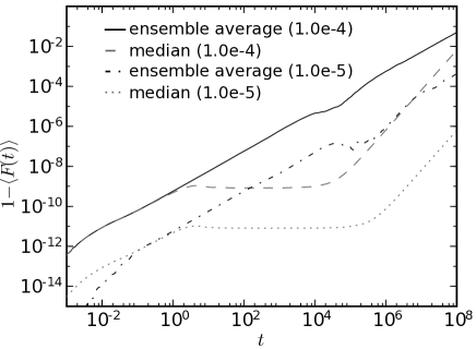
Figure 2: Average fidelity in $10^{5}$ realizations of $H_{0}$ and $V$ compared to the median fidelity for $6$ particles in $12$ orbitals and with two values of perturbation strengths $\lambda=10^{-4}$ and $\lambda=10^{-5}$. The median fidelity decay (long-dashed, dotted) shows a plateau practically absent in the ensemble average (full, short-dashed curves).

We therefore proceed to analyze the median of fidelity decay. For this purpose we use fidelity $F(t)=|f(t)|^{2}$, which is a real quantity, instead of fidelity amplitude $f(t)$. (We note however that the results are practically the same for the real part of fidelity amplitude.) We define median fidelity $F_{\textrm{m}}(t)$ such that at any time $F_{\textrm{m}}(t)$ is lower than fidelity $F(t)$ in half of the realizations. For a randomly chosen member of the ensemble there is thus a $0.5$ probability that a plateau in fidelity decay will last longer than the median fidelity plateau (Fig. 2).

A useful alternative in such situation is to consider the average of the logarithm of the quantity under consideration – in our case $\langle\ln(1-F(t))\rangle$. This quantity has been used in elastodynamics under the name distortion as we have discussed in the introduction. The distortion shown in figure 4 in the following section has essentially the same feature as the median. Note that it is not obvious how to obtain analytical results for either of these quantities, but the latter may be slightly more accessible.

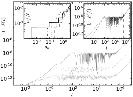
Figure 3: Fidelity decay in a few individual ensemble members for the residual case with $6$ particles and $12$ orbitals. The upper left inset shows a small region of the corresponding cumulative level spacing distribution of the unperturbed spectra $H_{0}$ (We plot a relative number of level spacing $n/{\cal N}$ below $s_{n}$.) The agreement with the minimum spacing only theory (dotted) is shown in the upper right inset, dashed line denotes the ending time $t_{\textrm{e}}$ (eq. (16).

It remains to be understood how the freeze, which is present in most realizations, comes about and is eventually completely averaged out. To elucidate this problem fidelity of a few individual ensemble members is presented (Fig. 3). However, the cases shown in the figure are not all equally probable; the upper one occurs rarely whereas the lower two curves truly represent the majority of cases. The upper left inset of Fig.3 shows the beginning of the cumulative level spacing distribution of $H_{0}$ corresponding to the fidelity curves shown in the main figure. Interestingly, the plateau properties of the exceptional large deviation cases with high plateaus are determined by the minimum energy spacing alone and the conjecture is that the plateau vanishes together with the smallest level spacing.

Another peculiarity results from the two-body nature of interaction which only connects certain levels as shown in section IV. Transitions involving three orbitals will very likely have big energy difference because of the level repulsion in single-particle spectra; this contrasts with the transitions involving four orbitals that can easily have small energy differences if one particle lowers the energy by roughly the same amount by which the other one raises it. The effect of a such two-body operator will be greater than the effect of any other operator.

Considering the established connection between the level spacing of four-orbital two-body operators and the fidelity amplitude plateau, an illustration is made where all three-orbital terms are omitted. Each four-orbital two-body operator $c_{i}^{\dagger}c_{j}^{\dagger}c_{l}c_{k}$ is in a unique way connected with the energy difference $\mu_{ijkl}:=e_{i}\!+\!e_{j}\!-\!e_{k}\!-\!e_{l}$ in the spectrum of $H_{0}$ and the four-orbital part of the correlation function (III) averaged over the perturbation becomes a sum over all possible positive spacings

$$C_{\alpha}(t) = v^{-2}\!\!\!\sum_{i<j\neq k<l}\Big{[}{\langle\alpha|}{\bar{n}_{i}}{\bar{n}_{j}}n_{l}n_{k}\mathrm{e}^{-2\pi\mathrm{i}|\mu_{ijkl}|}{|\alpha\rangle}$$ (12)

$$+ {\langle\alpha|}{\bar{n}_{k}}{\bar{n}_{l}}n_{j}n_{i}\mathrm{e}^{2\pi\mathrm{i}|\mu_{ijkl}|}{|\alpha\rangle}\Big{]}.$$

Assuming random initial states averaging can be performed

$$\frac{1}{\mathcal{N}}\sum_{\alpha}C_{\alpha}(t)=\frac{8(N-4)!}{N!(1+\frac{4}{N-M-1})}\sum_{q}\cos 2\pi\mu_{q}t$$ (13)

and the fidelity amplitude is obtained by integration (11) as

$$f(t)=1-\lambda^{2}\frac{8(N-4)!}{N!(1+\frac{4}{N-M-1})}\sum_{q}\frac{1-\cos 2\pi\mu_{q}t}{\mu_{q}^{2}}.$$ (14)

If the smallest degenerate spacing $\mu_{0}$ is orders of magnitude smaller than any other spacing, the sum above can be approximated by the smallest spacing term alone. All other terms are smaller by a factor $(\mu_{0}/\mu_{q})^{2}$. This approximation is very illustrative and can be used to estimate the beginning time $t_{\rm b}$ and the shift of the plateau by the condition $\mu_{0}t_{\rm b}=1$ and by removing the time-dependent part, respectively. Estimation of the ending time $t_{\rm e}$ of the plateau is a little more tedious. There we need the fourth-order terms in the linear response formula (2). Following the same principles and keeping the minimum spacing term only we obtain the fourth-order correction to fidelity of highest order in time (we are interested in very long times) as

$$f^{(4)}(t)=\frac{128\pi^{2}(N-4)!(N\!-\!M\!-\!1)}{N!(N\!-\!M)M(M\!-\!1)(N\!-\!M\!+\!3)^{2}}\frac{\lambda^{4}t^{2}}{\mu_{0}^{2}}.$$ (15)

The ending time $t_{\rm e}$ can then be estimated by comparing amplitudes of the second and fourth-order terms which gives the well knownfreezeint ; freezech $\lambda^{-1}$ dependence

$$t_{\rm e}=\frac{1}{2\pi\lambda}\sqrt{{M\choose 2}(N-M)(N-M+3)}.$$ (16)

The ending time does not depend on level spacings, which is again in agreement with the data shown in Fig. 3. If $t_{\rm b}\sim t_{\rm e}$ the plateau, which is a pure second-order phenomenon, would begin in the region where the second order approximation is no longer valid and hence cannot exist. The upper right inset on Fig. 3 shows that the second and fourth order terms together describe all important features of the fidelity amplitude decay for the uppermost realization in Fig 3 with an extremely small level spacing.

We now understand why the plateau, nearly always present in individual realizations, does not appear in the ensemble average. Realizations of the unperturbed spectrum with an extremely small level spacing occur rarely but when averaging the fidelity amplitude they eventually dominate the behavior and the plateaux are averaged out.

VI Comparison to other models

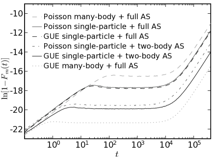
Figure 4: Median fidelity decay (left) and average natural logarithm of $1-F(t)$ (right) for various models (described in text and labeled in the figure - ordered from top to bottom) for $5$ particles in $10$ orbitals and perturbation strength $\lambda=10^{-4}$. Perturbation is always imaginary antisymmetric. The results are averaged over $2\cdot 10^{4}$ realizations.

The theory we have developed to describe the behavior of the model under consideration can be applied to other physical models and used to understand the differences between them. The key features of the model (4) are 1) level repulsion in single particle spectra and 2) sparse perturbation. By comparing to models with full random matrix spectra which correspond to chaotic dynamics on the one hand, and independent Poissonian spectra which corresponds to regular dynamics on the other hand, we find that our model lies somewhere in between as we can see from the Fig. 4. Besides the median fidelity which corresponds to the typical behavior, an alternative measure namely the average of the logarithm of $1-F(t)$ (also known a distortion) is considered in parallel. Although not completely identical, they both show essentially the same features and to some extent even quantitative agreement. In order to eliminate any potential effect of diagonal perturbation terms, we consider in the following models always purely imaginary antisymmetric perturbation, individually normalized in the usual way (${\rm tr}[V^{2}]=\mathcal{N}$). However, we will be switching between the cases of a full and a two-body perturbation matrix.

The first model under consideration (uppermost) has a random spectrum of $H_{0}$ such that the level spacing distribution is Poissonian. The perturbation is chosen from an ensemble of full antisymmetric matrices. The Poissonian level spacing distribution favors small spacings between spectral levels which contribute to fast (initially linear) fidelity decay. In this case the type of perturbation has no significant effect as small spacings are probable for any pair of levels. This is not true for $H_{0}$ constructed from independent single particle spectra which we take as Poissonian or GUE as in our original model (4). For the latter, small level spacing for some transitions (e.g. three-orbital two-body transitions) is very improbable. If the perturbation is a full matrix, the effect of such transitions is relatively small and there is no significant difference between the two cases. If, on the other hand, only a few levels are coupled as in the case of two-body interactions, three-orbital transitions in the case of Poissonian single particle spacings can and in the case of GUE spacings cannot involve small spacings. Thus in the former case they cannot be neglected. Typical decay of fidelity is in both cases slower than in the case of full perturbation. For illustration, also a completely different physical situation with random matrix many-body spectrum of $H_{0}$ is shown. Because of the level repulsion in many-body spectra, any transition will very unlikely have small level spacing. Only then, the plateau in fidelity decay is present not only in a typical case but also on average.

VII Ground state fidelity amplitude

Figure 5: Fidelity amplitude decay for the ground state and first excited state compared to higher excited state ${|s\rangle}$ (eq. (17)) for $6$ particles in $12$ orbitals and perturbation strength $\lambda=10^{-4}$. The results are averaged over $10^{4}$ realizations of perturbation and spectra.

We have up to now considered only random initial states, but the behavior of the ground state of the independent particle model $H_{0}$, i.e. the Hartree-Fock ground state, under a perturbation formed by residual interactions is also of interest. The correlation function can now no longer be simplified by state averaging. The main problem is to determine the matrix element $[V(t)V(0)]_{gg}=C_{g}(t)$ where ${|g\rangle}=c_{0}^{\dagger}\!\cdots\!c_{M-1}^{\dagger}{|0\rangle}$ is the ground state occupying the lowest $M$ single-particle levels. Regardless of the realization of the spectra of $H_{0}$, any non-diagonal two-body operator raises the energy for at least the minimum level spacing in the single-particle spectra where levels are unlikely to be close together. The same incidentally holds in the first excited state with the only difference that there the energy can also be lowered by the same amount. Note that more freedom does exist for higher excited states such as for example

$${|s\rangle}=c_{0}^{\dagger}\!\cdots\!c_{M-2}^{\dagger}c_{M}^{\dagger}c_{M+1}^{\dagger}{|0\rangle}$$ (17)

where the operator $c_{M-1}^{\dagger}c_{M+2}^{\dagger}c_{M+1}c_{M}$ or its hermitian conjugate increases or decreases energy by $e_{M-1}+e_{M+2}-e_{M}-e_{M+1}=(e_{M+2}-e_{M+1})-(e_{M}-e_{M-1})$ which indeed can be very small.

This leads to the suspicion that the freeze might exist on average for these two lowest independent particle initial states. The numerical results indeed show (Fig. 5) the plateau in the ensemble averaged fidelity amplitude for the ground and the first excited state.

VIII Conclusion

We have analyzed a very elementary many-fermion model in context of echo dynamics. The model describes spinless fermions whose underlying single-particle dynamics is chaotic and are perturbed by random two-body interactions. Our interest was focused on the stability of a mean field approximation where the diagonal terms of the interaction have been included in the unperturbed Hamiltonian. For weak perturbations the decay of the fidelity amplitude in this case typically displays a high-level plateau also known as freeze of fidelity. This freeze lasts for times long on the scale of the Heisenberg time. The unexpected point is that the freeze typically present in most realizations of members of the ensemble will vanish on average giving a very dramatic example of the non-ergodicity of the TBRE. To see the effect which should dominate most experiments and should hence be observable, we have to consider median behavior or consider logarithmic averages. This fact beyond the specific interest for the TBRE could pave the road for interesting new applications of random matrix theory analyzing non-ergodic situations.

*

Appendix A Analytical calculation of the correlation function

The final compact expression for the averaged correlation function $C(\tau)$ (see eq. 10) involves Fourier integrals of the Dyson’s correlation functions $R_{n}(\mathbf{x})$

$$\mathcal{F}[R_{n}](k)=\frac{(N\!-\!n)!}{N!}\int_{-\infty}^{\infty}\!\!\!R_{n}(\mathbf{x})\mathrm{e}^{-\mathrm{i}k\sum_{j=0}^{n-1}(-1)^{j}x_{j}}\mathrm{d}^{n}\mathbf{x}.$$ (18)

If the correlations functions $R_{n}$ correspond to GUE, such integrals can be analytically integrated and presented in terms of functions $J_{nm}(t)$:

$$J_{nm}(t)=\int_{-\infty}^{\infty}H_{n}(x)\mathrm{e}^{-x^{2}}H_{m}(x)\mathrm{e}^{-\mathrm{i}tx}\mathrm{d}x$$ (19)

where $H_{n}(x)$ are standard Hermite polynomials. It can easily be shown using recursion that a function $J_{mn}(t)$ can be written as finite series

$$J_{mn}(t)=\frac{\mathrm{e}^{-t^{2}/4}(-\mathrm{i}t)^{n+m}}{\sqrt{2^{n+m}n!m!}}\sum_{j=0}^{\textrm{min}(m,n)}\!\!\!(-2)^{j}j!{m\choose j}{n\choose j}\frac{1}{t^{2j}}.$$ (20)

The simplest case is the transformation of $R_{1}(x)=\sum_{n=0}^{N-1}\frac{1}{2^{n}n!\sqrt{\pi}}\mathrm{e}^{-x^{2}}H_{n}(x)^{2}$ which gives a simple result

$$\mathcal{F}[R_{1}](t)=\sum_{n=0}^{N-1}J_{nn}(t).$$ (21)

Higher level correlation functions $R_{n}$ are expressible by lower level $R_{n}$ and cluster functions $T_{2}$ mehtabook . Because $\mathcal{F}$ is a linear transformation it can also be expressed by lower order transformations where transformations of cluster functions involve terms without the sign factors $(-1)^{j}$ in the exponential in (18), denoted by $\mathcal{F}[T_{n}]^{+}$. Straight-forward calculation gives

$$\mathcal{F}[T_{2}]^{\mp}(t) = \sum_{nm}J_{nm}(t)J_{nm}(\mp t)$$ (22)

$$\mathcal{F}[T_{3}]^{\mp}(t) = \sum_{nmk}J_{mn}(t)J_{mk}(-t)J_{nk}(-t)$$ (23)

$$\mathcal{F}[T_{4}]^{\mp}(t) = \sum_{mnkl}J_{ml}(t)J_{mn}(t)J_{kl}(-t)J_{nk}(-t).\quad\quad$$ (24)

Finally, following the equality $R_{2}(x,y)=R_{1}(x)R_{1}(y)-T_{2}(x,y)$ and similarly for $R_{4}$ it finally holds

$$\mathcal{F}[R_{2}](t) = \mathcal{F}[R_{1}](t)^{2}-\mathcal{F}[T_{2}]^{-}(t)$$ (25)

$$\mathcal{F}[R_{4}](t) = \mathcal{F}[R_{1}](t)^{4}+\mathcal{F}[T_{2}]^{+}(t)^{2}+2\mathcal{F}[T_{2}]^{-}(t)^{2}$$ (26)

$$- 2\mathcal{F}[R_{1}](t)^{2}\mathcal{F}[T_{2}]^{+}(t)-4\mathcal{F}[R_{1}](t)^{2}\mathcal{F}[T_{2}]^{-}(t)$$

$$+ 8\mathcal{F}[R_{1}](t)\mathcal{F}[T_{3}](t)-6\mathcal{F}[T_{4}](t).$$

Hence, the averaged correlation function, although not as a compact expression, can be analytically evaluated using the above equations.

References

- (1) E. P. Wigner, Ann. Math. 53, 36 (1951); E. P. Wigner, Proc. Cambridge Philos. Soc. 47, 790 (1951).
- (2) E. Cartan, Abh. Math. Sem. Univ. Hamburg 11, 116 (1935).
- (3) T. Brody et al., Rev. Mod. Phys. 53, 385 (1981).
- (4) R. Balian, Nuovo Cimento B57, 183 (1958).
- (5) T. Guhr, A. Müller-Groeling, and H. A. Weidenmüller, Phys. Rep. 299, 189 (1998).
- (6) J. French and S. Wong, Phys. Lett. 33B, 449 (1970).
- (7) O. Bohigas and J. Flores, Phys. Lett. 34B, 261 (1971).
- (8) J. B. French and S. S. M. Wong, Phys. Lett. 35B, 5 (1971).
- (9) L. Benet and H. A. Weidenmüller, J. Phys. A: Math. Gen. 36, 3569 (2003).
- (10) C. W. Johnson, G. F. Bertsch, and D. J. Dean, Phys. Rev. Lett. 80, 2749 (1998); C. W. Johnson, G. F. Bertsch, D. J. Dean, and I. Talmi, Phys. Rev. C 61, 014311 (1999).
- (11) T. Papenbrock and H. A. Weidenmüller, Nucl. Phys. A 575, 422 (2005).
- (12) R. Bijker, A. Frank, and S. Pittel, Phys. Rev. C 60, 021302 (1999).
- (13) J. B. French, Rev. Mex. Fis. 22, 221 (1973).
- (14) V. Zelevinsky, B. A. Brown, N. Frazier, and M. Horoi, Phys. Rep. 276, 85 (1996).
- (15) J. Flores, M. Horoi, M. Müller, and T. H. Seligman, Phys. Rev. E 63, 026204 (2000).
- (16) V. K. B. Kota, Phys. Rep. 347, 223 (2001).
- (17) A. Peres, Phys. Rev. A 30, 1610 (1984).
- (18) M. A. Nielsen and I. L. Chuang, Quantum Computation and Quantum Information (Cambridge University Press, Cambridge, 2000).
- (19) T. Gorin, T. Prosen, T. H. Seligman, and M. Žnidarič, Phys. Rep. 435, 33 (2006).
- (20) R. F. Jalabert and H. M. Pastawski, Phys. Rev. Lett. 86, 2490 (2001).
- (21) F. Cucchietti, C. Lewenkopf, E. Mucciolo, H. Pastawski and R. Vallejos, Phys. Rev. E 65, 046209 (2002).
- (22) F. M. Cucchietti, D. A. R. Dalvit, J. P. Paz, and W. H. Zurek, Phys. Rev. Lett. 91, 210403 (2003).
- (23) J. Vanicek and E. Heller, Phys. Rev.E 68, 056208 (2003); J. Vanicek, Phys. Rev. E 70, 055201(R), (2004); ibid. 73, 046204 (2006).
- (24) H.-J. Stöckmann and R. Schäfer, New J. Physics 6, 199 (2004).
- (25) H.-J. Stöckmann and H. Kohler, Phys. Rev. E 73, 066212 (2006).
- (26) T. Gorin, T. Prosen, and T. H. Seligman, New J. of Physics 6, 20 (2004).
- (27) T. Prosen, Phys. Rev. E 65, 036208 (2002).
- (28) T. Prosen and M. Žnidarič, J. Phys. A 35, 1455 (2002).
- (29) T. Prosen, T. H. Seligman, and M. Žnidarič, Prog. Theor. Phys. Suppl. 150, 200 (2003).
- (30) T. Gorin et al., Phys. Rev. Lett. 96, 244105 (2006).
- (31) Ph. Jacquod, P. G. Silvestrov, and C. W. J. Beenakker, Phys. Rev. E 64, 055203(R) (2001).
- (32) N. R. Cerruti and S. Tomsovic, Phys. Rev. Lett. 88, 054103 (2002).
- (33) T. Prosen and M. Žnidarič, New J. Phys. 5, 109 (2003).
- (34) T. Prosen and M. Žnidarič, Phys. Rev. Lett. 94, 044101 (2005).
- (35) O. I. Lobkis and R. L. Weaver, Phys. Rev. Lett 90, 254302 (2003).
- (36) T. Gorin, T. H. Seligman, and R. L. Weaver, Phys. Rev. E 73, 015202(R) (2006).
- (37) F. Leyvraz, 2006, private communication.
- (38) V. V. Flambaum, G. F. Gribakin, and F. M. Izrailev, Phys. Rev. E 53, 5729 (1996); V. V. Flambaum and F. M. Izrailev, Phys. Rev. E 61, 2539 (2000).
- (39) Y. Alhassid, Ph. Jacquod, and A. Wobst, Phys. Rev. B 61, R13357 (2000).
- (40) F.-M. Dittes, I. Rotter, and T. H. Seligman, Phys. Lett. A 158, 14 (1991).
- (41) M. L. Mehta, Random Matrices (Revised and Enlarged, 2nd Edition) (Academic Press, London, 1991).