Thermodynamic Entropy and Chaos in a Discrete Hydrodynamical System

Abstract

We show that the thermodynamic entropy density is proportional to the largest Lyapunov exponent (LLE) of a discrete hydrodynamical system, a deterministic two-dimensional lattice gas automaton. The definition of the LLE for cellular automata is based on the concept of Boolean derivatives and is formally equivalent to that of continuous dynamical systems. This relation is justified using a Markovian model. In an irreversible process with an initial density difference between both halves of the system, we find that Boltzmann’s $H$ function is linearly related to the expansion factor of the LLE, although the latter is more sensitive to the presence of traveling waves.

I Introduction

The relation between thermodynamics and the underlying chaotic properties of a system is of great relevance in the foundations of statistical mechanics lebowitz73 ; zaslavsky04 and has attracted much interest. What is the relation between chaotic dynamics and thermodynamics? Is chaos relevant for thermodynamics? Some interesting results have been found for some models. In the case of a family of simple liquids, including Lennard–Jones, a relation has been found between the Kolmogorov–Sinai entropy and the thermodynamic entropy dzugutov98 . Lorentz gases have been extensively studied and relationships between chaotic dynamical properties and transport coefficients have been established gaspard90 ; evans90 ; gaspard95 ; dorfman97 ; dorfman02 . The discussion of this problem for other simple models and maps is extensive gaspard97 ; latora99 ; tasaki99 ; gilbert00 ; tasaki00 .

Lorentz gases are essentially one-particle systems. In this paper we present a simple model of a gas with a large number of interacting particles and find interesting relations between dynamic and thermodynamic quantities, somewhat motivated by Bernoulli systems. For these, the Kolmogorov-Sinai entropy is on the one hand the sum of the positive Lyapunov exponents, and on the other, the thermodynamic entropy scaled by a time constant corresponding to the correlation time billingsley82 ; cornfeld82 .

The model we study is a deterministic lattice gas cellular automaton (LGCA). LGCA are simple models with hydrodynamical behavior hardy73 ; frisch86 ; frisch87 . In particular, the $D2Q9$ LGCA is a two dimensional model with nine velocities and is one of the simplest models where equilibrium thermodynamics can be found with a non trivial temperature bagnoli93 . For cellular automata, Lyapunov exponents can be defined using Boolean derivatives bagnoli92 . This definition is formally similar to that of continuous dynamical systems, a long time average of the logarithm of the linearized expansion factor ott93 . We also look for a relation between Boltzmann’s $H$ function in a simple irreversible process, and the logarithm of the expansion factor.

The paper is organized as follows. In Sec. II we present a deterministic version of the $D2Q9$ model together with an introduction to Lyapunov exponents of cellular automata. In Sec. III we discuss the equilibrium thermodynamics of the $D2Q9$ models and in Sec. IV we show there is a close relationship between the equilibrium entropy of the model and its largest Lyapunov exponent. This relationship is explained by finding the Kolmogorov-Sinai entropy of a Markov chain which relates the thermodynamic entropy to the largest Lyapunov exponents. We also show that Boltzmann’s $H$ function goes to its equilibrium value in an irreversible process in the same way the Lyapunov exponent does. We end with a discussion on why these quantities are related.

II The $D2Q9$ model

The $D2Q9$ model is defined on a two dimensional square lattice chen89 . The evolution is in discrete time steps where unit mass particles at every site ${\bm{r}}$ can move with one of nine velocities ${\bm{c}}_{0}=(0,0)$, ${\bm{c}}_{1}=(1,0)$, ${\bm{c}}_{2}=(0,1)$, ${\bm{c}}_{3}=(-1,0)$, ${\bm{c}}_{4}=(0,-1)$, ${\bm{c}}_{5}=(1,1)$, ${\bm{c}}_{6}=(-1,1)$, ${\bm{c}}_{7}=(-1,-1)$, ${\bm{c}}_{8}=(1,-1)$. The state of the automaton is given by the set of occupation numbers ${\bm{s}}(t)=\{s_{k}({\bm{r}},t)\}$, where $s_{k}({\bm{r}},t)=1$ (0) indicates the presence (absence) of a particle with velocity ${\bm{c}}_{k}$ at site ${\bm{r}}$ and time $t$. An exclusion principle forbids the presence of more than one particle in a given site and a given time with a given velocity.

The time evolution of the system is given by collision and streaming operations. In the collision step, the particles at every site change their velocities conserving mass, momentum and energy. In the streaming operation particles move to neighboring sites according to their velocities.

Figure 1: All these states have the same number of particles, momentum and energy. An arrow represents the presence of a particle with the velocity of the arrow, the open circle a particle at rest.

Since the number of states for a given site is finite ($2^{9}$), the local collision operator $C$ is generally implemented as a look-up table. Given a local configuration, the conservation constraints may not define the outgoing state completely as the example in Fig. 1 shows. If any one of the six states shown is chosen as the input state, any one of the other six states can be the output state. Therefore, the $C$ look-up table has several columns for all the possible output states. In order to make the automaton deterministic, we first find for all input states, the number of output states. We then find the least common multiplier of the number of output states and construct a new $C$ look-up table with this number of columns. These are filled by repeating the output states the required number of times. The least common multiplier is sixty, so the rows which have any one of the input states of Fig. 1 are repeated ten times. At the beginning we assign an integer random number $\eta({\bm{r}})$ to each site, to be used in choosing the column from which the output state is chosen (quenched disorder). That is

$$s_{k}({\bm{r}},t+1)=C_{k}(s_{0}({\bm{r}},t),\dots,s_{8}({\bm{r}},t),\eta({\bm{r}})).$$ (1)

The choice of the quenched disorder is analogous to the random disposition of scatterers in a wind-tree or other similar Lorentz gases ehrenfest11 ; ernst89 .

The evolution of the model can also be made reversible. In order to do so, the collision table must satisfy the condition that in every column $s={\bm{I}}{\bm{C}}{\bm{I}}{\bm{C}}(s)$ holds where ${\bm{I}}$ denotes the operator that inverts the velocities of any state $s$. This means that a collision ${\bm{C}}$ followed by an inversion ${\bm{I}}$ and another collision and inversion leaves the state unchanged when it is taken from the same column in the collision table as we show in Fig. 2. Once we have a look-up table that is deterministic as described above, the elements in each row are rearranged to satisfy the reversibility condition.

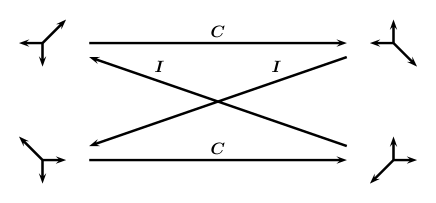
Figure 2: In this example, the input state at some fixed site is the one shown on the left of Fig. 1 and in the column number assigned to this site, the output state is the fourth one of that Fig. These are shown in the upper part of this Fig. Then, by inverting the velocities we get the state on the lower left and the collision table should contain in the same column for this input state the output state shown on the lower right that upon inversion of the velocities yields the original incoming state.

In order to introduce the concept of Lyapunov exponents for such a system, it is convenient to simplify the notation used. We use the index $n$ to indicate the position ${\bm{r}}$ and the velocity $k$, with $n=1,\dots,9L$, where $L$ is the number of sites of the automaton. A configuration of the LGCA at a given time is given by $9L$ occupation numbers (bits), and its evolution can be seen as an application of a set of Boolean functions

$${}s_{n}(t+1)=F_{n}({\bm{s}}(t)).$$ (2)

The functions $F_{n}$ represent different entries of the collision table, and differ in the velocity index $k$ and quenched disorder $\eta({\bm{r}})$. However, since the distribution of the disorder is uniform, and, as shown in the following, the correlations among variables decay very fast, the system is translationally invariant at a mesoscopic level.

Let ${\bm{s}}(0)$ and ${\bm{x}}(0)$ be two initially close configurations, for example all the components of ${\bm{x}}(0)$ may be equal to those of ${\bm{s}}(0)$ except for one. We define the bitwise difference between these two configurations with the term “damage”. The smallest possible damage is one and the damage vector ${\bm{v}}(0)$ has a one in the component where ${\bm{s}}(0)$ and ${\bm{x}}(0)$ differ and has zeroes in all the others. If this damage grows on average during time, the trajectory is unstable with respect to the smallest perturbation. However, due to the discrete nature of LGCA, defects may annihilate during time evolution, altering the measure of instability of trajectories. The correct way of testing for instability is that of considering all possible ways of inserting the smallest damage in a configuration, using as many replicas as the number of components of the configuration, and letting them evolve for one time step counting if the number of damages has grown or diminished. The ensemble of all possible replicas with one damage each is the equivalent of the tangent space of discrete systems.

The task of computing the evolution in tangent space is clearly daunting, but by exploiting the concept of Boolean derivatives bagnoli92 ; bagnoli92a it is possible to develop a formula very similar to the one used in continuous systems. The Boolean derivative is defined by

$$\dfrac{\partial F_{n}({\bm{s}})}{\partial s_{p}}=\left|F_{n}(\dots,s_{p},\dots)-F_{n}(\dots,1-s_{p}\dots)\right|$$ (3)

with $n,p=1,\dots,9L$. This quantity measures the sensitivity of the function $F_{n}$ with respect to a change in $s_{p}$. The Jacobian matrix $J({\bm{s}})$ has components $J_{np}=\partial F_{n}({\bm{s}})/\partial s_{p}$.

We now consider the map

$${\bm{v}}(t+1)=J({\bm{s}}(t)){\bm{v}}(t)$$ (4)

with ${\bm{v}}(0)$ as mentioned above. It is easy to check that $|{\bm{v}}(t)|=\sum_{i}v_{i}(t)$ is the number of different paths along which a damage may grow in tangent space during time evolution, i.e., with the prescription of just one defect per replica bagnoli92 . If there is sensitivity with respect to initial conditions, one expects that $|{\bm{v}}(T)|/|{\bm{v}}(0)|\sim\exp(\lambda_{{}_{T}}T)$ for large $T$ where $\lambda_{{}_{T}}$ is the largest finite time Lyapunov exponent (LLE). It then follows that

$$\lambda_{{}_{T}}=\dfrac{1}{T}\sum_{t=1}^{T-1}\log u(t)=\langle\log u\rangle_{{}_{T}}$$ (5)

with $u(t)=|{\bm{v}}(t)|/|{\bm{v}}(t-1)|$ the expansion factor of the LLE. The definition should include the limit when $T\to\infty$ but in practice we always evaluate the finite time LLE with $T$. The LLE depends in principle on the initial configuration ${\bm{s}}(0)$, initial damage ${\bm{v}}(0)$ and quenched disorder $\eta$, but in practice it assumes the same value for all trajectories corresponding to the same macroscopic observables when $T$ is sufficiently large. The LLE of CA as defined above has been used to classify elementary and totalistic Boolean cellular automata bagnoli92 ; bagnoli94 .

III Thermodynamics of the $D2Q9$ model

The single particle velocity distribution functions $f_{k}({\bm{r}},t)$ are defined as the average number of particles at site ${\bm{r}}$ with velocity ${\bm{c}}_{k}$ at time $t$ over $R$ samples that share the same quenched disorder $\eta$ and macroscopic constraints with different microscopic initial configurations.

We checked that the single site two-particle correlation function factorizes into the product of single particle distributions before and after the collision, in equilibrium and out of equilibrium conditions. In equilibrium, the correlation function decays to zero for just one lattice spacing. Out of equilibrium, starting with very different configurations in the two halves of the system, the correlation function, still being quite small, exhibits a correlation length of some lattice spacings for a short time. This corresponds to the coherent motion of particles in a shock wave, where the local density is near to zero or nine. However, this correlation quickly disappears; although the motion is correlated at a macroscopic level, as soon as the local density of particles is different from the extremes (for which the collision table has few output configurations) the velocities quickly decorrelate.

The thermodynamic entropy density can be found analytically in the thermodynamic limit as follows salcido91 . Let

$$N=\sum_{k}N_{k},\qquad E=\sum_{k}\epsilon_{k}N_{k}$$ (6)

with $N$ and $E$ the number of particles and total energy respectively, $N_{k}$ the number of particles in direction $k$, and $\epsilon_{0}=0$, $\epsilon_{1,2,3,4}=1/2$, $\epsilon_{5,6,7,8}=1$. The number density $n$, the equilibrium density functions $f_{k}$ and the energy density $e$ are

$$n=\dfrac{N}{L},\qquad f_{k}=\dfrac{N_{k}}{L},\qquad e=\dfrac{E}{L}$$ (7)

with $L$ the number of sites in the lattice. The microcanonical partition function $\Omega$ is

$$\Omega=\int\prod_{k}dN_{k} \delta(N-\sum_{k}N_{k})\delta(E-\sum_{k}\epsilon_{k}N_{k})\times$$

$$\omega(N_{0},\dots,N_{8})$$ (8)

with $\delta$ the Dirac-$\delta$ function and

$$\omega=\prod_{k}\dfrac{L!}{N_{k}!(L-N_{k})!}.$$ (9)

the number of microscopic states in Fermi-Dirac statistics.

The thermodynamic entropy is $S(E,N,L)=\log\Omega(E,N,L)$. Using Stirling’s approximation and the Fourier transform of the $\delta$ function

$$S=\log\left(L^{9}\int\prod_{k}df_{k}\int dp_{1}dp_{2}\exp(L\sigma)\right)$$ (10)

with

$$\sigma= -\sum_{k}\left[f_{k}\log f_{k}+(1-f_{k})\log(1-f_{k})\right]$$

$$+ip_{1}\left[n-\sum_{k}f_{k}\right]+ip_{2}\left[e-\sum_{k}\epsilon_{k}f_{k}\right].$$ (11)

The integrals of Eq, (10) can be evaluated using the saddle point method and the result is exact in the thermodynamic limit. The thermodynamic limit entropy density $s$ is

$$s(e,n) =\lim_{L\to\infty}\dfrac{1}{L}S(eL,nL,L)$$

$$=-\sum_{k}\left[\hat{f}_{k}\log\hat{f}_{k}+(1-\hat{f}_{k})\log(1-\hat{f}_{k})\right].$$ (12)

In the last expression $\hat{f}_{0},\dots\hat{f}_{8},\hat{p}_{1}$, and $\hat{p}_{2}$ maximize $\sigma$ given by Eq. (11).

The quantities $p_{1}$ and $p_{2}$ are related to temperature and chemical potential. Taking the partial derivative of $\sigma$ with respect to $f_{k}$ and equaling to zero we find that

$$\log\left(\dfrac{\hat{f}_{k}}{1-\hat{f}_{k}}\right)=-i\hat{p}_{1}-i\hat{p}_{2}\epsilon_{k},$$ (13)

and that

$$\hat{f}_{k}=\left[1+\exp(i\hat{p}_{1}+i\hat{p}_{2}\epsilon_{k})\right]^{-1}.$$ (14)

Using Eq. (13) the entropy density is

$$s=-\sum_{k}\left(\log(1-\hat{f}_{k}\right)+i\hat{p}_{1}+i\hat{p}_{2}\epsilon_{k}.$$ (15)

The Euler equation is

$$s=\dfrac{e}{T}+\dfrac{P}{T}-\dfrac{\mu N}{T}$$ (16)

where $P$ is the pressure and $\mu$ is the chemical potential. Comparing the last two expressions

$$\dfrac{1}{T} =i\hat{p}_{2},$$ (17)

$$-\dfrac{\mu}{T} =i\hat{p}_{1},$$ (18)

$$\dfrac{P}{T} =-\sum_{k}\log(1-\hat{f}_{k}).$$ (19)

Now, the equilibrium distribution functions are

$$\hat{f}_{k}=\left[1+\exp(\epsilon_{k}/T-\mu/T)\right]^{-1}.$$ (20)

The distribution functions $\hat{f}_{0}$, $\hat{f}_{1}$, and $\hat{f}_{5}$ define the equilibrium state since $\hat{f}_{1}=\hat{f}_{2}=\hat{f}_{3}=\hat{f}_{4}$ and $\hat{f}_{5}=\hat{f}_{6}=\hat{f}_{7}=\hat{f}_{8}$. These satisfy the conservation equations of mass end energy and maximize $\sigma$. We also note that these distributions satisfy another condition equivalent to the latter. From Eq. (13) for $k=1,5$ and for $k=0$ and Eq. (18)

$$\dfrac{\mu}{T}=\log\left(\dfrac{f_{0}}{1-f_{0}}\right)=\log\left(\dfrac{f_{1}}{1-f_{1}}\right)^{2}\left(\dfrac{1-f_{5}}{f_{5}}\right).$$

Then

$$f_{1}^{2}(1-f_{0}-f_{5})=f_{0}f_{5}(1-2f_{1}).$$ (21)

This last expression, together with mass and energy conservation determine the equilibrium values of the distribution functions. In Fig. 3 we show the values of the equilibrium distribution functions as continuous curves, together with result of numerical simulations. The agreement between numerical simulations and computed values of the probability distributions is perfect, and this confirms that the system is a perfect gas. Further investigations on correlations in out of equilibrium conditions are reported in the following Section.

Figure 3: Distribution functions in equilibrium as a function of $e$ for $n=4$. The continuous curves are the calculated values, the symbols are the results of numerical simulations. For $e=e_{F}$ there is a rest particle in all sites and no fast particles moving along the diagonals. The other three particles can occupy one of the four slow directions. For $e=e_{M}$ there are no rest or slow particles, the four particles are moving along the diagonals.

IV Results and discussion

In Fig. 4 we show the entropy density $s=S/L$ and the LLE $\lambda$ as a function of $e$ for fixed $n$ both calculated numerically. The entropy density is found by substituting the numerical values of $f_{k}$, for example those of Fig. 3, in Eq. (12). The entropy density grows for $e_{\text{F}}\leq e\leq e^{\ast}$ and then decreases for $e^{\ast}\leq e\leq e_{\text{M}}$ with $e^{\ast}=2n/3$. The energy density $e^{\ast}$ is the value for which $f_{0}=f_{1}=f_{5}$. The largest Lyapunov exponent $\lambda$ shows the same behavior having a maximum also at $e^{\ast}$. The results shown suggest that $s$ is proportional to $\lambda$. This is emphasized in Fig. 5 where the data lie near a straight line for different values of $n$. This result shows that the LLE grows with the number of available states measured by the equilibrium entropy.

Figure 4: Entropy density $s$ (solid line) and LLE $\lambda$ (dashed line) for $n=4$, simulations with $R=40$ in a $40\times 40$ lattice.

Figure 5: We show $s$ versus $\lambda$ for $n=2$ (diamonds), $n=4$ (solid line), $n=4.5$ (dotted line) and $n=6$ (pluses). The simulations are performed for different values of $e$ from $e_{\text{F}}(n)$ to $e_{\text{M}}(n)$.

The proportionality between the thermodynamic entropy density and the largest Lyapunov exponent can be understood in the framework of the stochastic approximation of a chaotic dynamics dorfman99 . In this approximation, the dynamics is considered at discrete time intervals, and generates a discrete and finite partition of coarse-grained states labeled by an index $i$, with $i=1,\dots,M$. The evolution is represented by a Markov chain where $W_{ij}$ is the transition probability from state $j$ to state $i$ and $\sum_{i}W_{ij}=1$. The asymptotic probability distribution is denoted by $p_{i}$, with $\sum_{i}p_{i}=1$ and $\sum_{j}W_{ij}p_{j}=p_{i}$. The Kolmogorov-Sinai entropy $K$ per time interval $\tau$ is dorfman99 ; ott93

$$K=-\sum_{j}p_{j}\sum_{i}W_{ij}\log W_{ij},$$ (22)

and the entropy density $s$ is

$$s=-\sum_{i}p_{i}\log p_{i}.$$ (23)

For Bernoulli systems the equilibrium is reached in just one time step, $W_{ij}=p_{j}$, and trivially $K=\tau^{-1}s$ gaspard93 . For a somewhat more general process, we assume that $p_{i}=1/M$ (microcanonical distribution) so that $s=\log M$. We further assume that the transition matrix is irreducible (so that the system is ergodic) and that in each row and column there are $\alpha_{i}M$ non zero equal entries with values $1/\alpha_{i}M$, $0<\alpha_{i}\leq 1$. Then

$$K=\langle\log\alpha\rangle+\log M,$$ (24)

where $\langle\log\alpha\rangle$ is the average of $\log\alpha_{i}$.

If we further assume the validity of the Pesin relation pesin77 , $K$ equals the sum of positive Lyapunov exponents. For many Hamiltonian systems and symplectic maps, the Lyapunov spectrum takes the form $\lambda_{i}\simeq\lambda_{0}(1-i/(2N))$, where $\lambda_{i}$ is the $i$-th Lyapunov exponent, $i=0,\dots,2N-1$ and the number of particle $N$ is large. In these cases, the Kolmogorov-Sinai entropy per degree of freedom is proportional to the largest Lyapunov exponent $\lambda_{0}$. The proportionality constant, however, may depend on the value of control parameters, namely the energy.

The shape of the Lyapunov spectrum is roughly linear for the product of random matrices with the structure of (weakly) locally coupled Hamiltonian chaotic systems paladin86 and for coupled nonlinear oscillators ruffo86 .0 If we assume that also in other cases the shape of the spectrum (which in general is not linear, see for instance Ref. beijren04 for the hard spheres case) does not change with the energy, it follows that $s$ and $\lambda$ are linearly related. This last assumption is probably the weakest one, at least for LGCA for which the Lyapunov spectrum is ill-defined, and we think it is the main reason for the discrepancy from linearity in Figure 5.

Figure 6: Boltzmann function $H$ (thick line) and Lyapunov expansion factor $\langle\ell\rangle$ (oscillating thin line) versus time $t$, simulations with $n_{L}=7.2$, $e_{L}=4.8$, $n_{R}=1.8$, $e_{R}=1.2$, and $R=40$ on a $40\times 40$ lattice. The inset shows that, disregarding the oscillations of $\langle\ell\rangle$, there is a linear relation between these quantities. The dashed line is the best fit $H=1.15\langle\ell\rangle+0.2$.

In our model, the value of the LLE is related to the number of ones in the Jacobian matrix $J$ defined by Eq. (3). This Jacobian matrix contains the linearized effects of the streaming and collision operators. Streaming corresponds to a scrambling of the components of the tangent vector ${\bm{v}}(t)$ and therefore does not alter its norm. This is left to collisions, when more than one output configurations are possible. The number of equivalent output configurations in the collision table is small for the extreme values of number and energy densities, and larger for intermediate values. Similar considerations apply to the number of equivalent configurations for a given macroscopic distribution of density and velocities, and constitute the microscopic origin of the relation between statistical and dynamical quantities.

We now discuss an irreversible process where a square lattice is initially in an equilibrium state with the left and right sides having different number and energy densities $n_{L}$, $n_{R}$, $e_{L}$, and $e_{R}$. The system evolves toward equilibrium by means of damped traveling waves. The single site two-particle correlation function, although small, exhibits a correlation length of some lattice spacings for a short time.

Macroscopically, one observes a coherent motion of particles in a shock wave, where the local density is near zero or nine. Although the motion is correlated at a macroscopic level, as soon as the local density of particles is different from the extremes (for which the collision table has few output configurations) the velocities quickly decorrelate.

Boltzmann’s $H$ function is defined by

$$H(t)=-\sum_{{\bm{r}},k}f_{k}({\bm{r}},t)\log f_{k}({\bm{r}},t).$$ (25)

In the numerical simulations the distribution functions are averaged over $R$ samples and the average Lyapunov expansion factor is $\langle\ell\rangle=(1/R)\sum_{i=1}^{R}\log u^{(i)}$. As we show in Fig. 6, the two quantities exhibit similar behavior. The Lyapunov expansion factor exhibits more marked oscillations, indicating that it is more sensible to the local variations in density. The inset of Fig. 6 shows that, disregarding oscillations, $\langle\ell\rangle$ is linearly related to $H$ for all the relaxation phase.

We can identify several time scales in this irreversible process. There is a fundamental time scale, which is fixed to unity. There is also a correlation time scale, which is of the order of the mean free time which depends on the occurrence of non-trivial collisions and is larger where the density is either small or large. During shock waves, locally one may have variations of the density and therefore correlations, as already reported, of the order of some time steps. A third time scale is given by the oscillations induced by the traveling shock waves. This is a dynamical, mesoscopic scale, that depends on the size of the system, and is revealed by the oscillations of $\langle\ell\rangle$ shown in Fig. 6. The slowest time scale is given by the relaxation to equilibrium, shown both by $H$ and by $\langle\ell\rangle$.

The computation of $\langle\ell\rangle$ is performed using a set of tangent vectors, Eq. (4), and these vectors constitute a sort of local memory of the past state. In systems with local variations of density, as in our system in the presence of traveling waves, statistical quantities like $H$ depend on the instantaneous state of the system, while dynamical ones like $\langle\ell\rangle$ depend also on the variations of this state. This factor may be the origin of the different relation between statistical and dynamical quantities in equilibrium and during the relaxation phase.

V Final remarks

The $D2Q9$ reversible LGCA model we have discussed exhibits hydrodynamical and thermodynamical behavior. For this model, the thermodynamic entropy density is proportional to the largest Lyapunov exponent. Also, in a simple irreversible process, Boltzmann’s $H$ function is proportional to the expansion factor of the largest Lyapunov exponent. A simple stochastic coarse grained dynamics can explain the proportionality between $s$ and $\lambda$. We note that this result does not depend on the $D2Q9$ dynamics and should hold for other, possibly more realistic models. Finally, the fact that the thermodynamic entropy density and the LLE of the model are proportional confirms that the definition of the latter is appropriate.

References

- (1) J. Lebowitz, Phys.Today, September 1973, p. 32.
- (2) G. M. Zaslavsky, Phys. Today, August 2004, p. 39.
- (3) M. Dzugutov, E. Aurell, A. Vulpiani, Phys. Rev. Lett. 81 1762 (1998).
- (4) P. Gaspard, G. Nicolis, Phys. Rev. Lett. 65, 1693, (1990).
- (5) D. J. Evans, G. P. Morris, Statistical Mechanics of Nonequilibrium Liquids, (Academic Press, London 1990). W. G. Hoover Computational Statistical Mechanics, (Elsevier, Amsterdam, 1991).
- (6) P. Gaspard, J. R. Dorfman, Phys. Rev. E 52, 3525 (1995).
- (7) J. R.Dorfman, H. van Beijeren, Physica A 240, 12 (1997).
- (8) J. R. Dorfman, P. Gaspard, T. Gilbert, Phys. Rev. E 66, 026110 (2002).
- (9) P. Gaspard, J. Stat. Phys. 88 1215 (1997).
- (10) V. Latora and M. Baranger, Phys. Rev. Lett. 82, 520 (1999).
- (11) S, Tasaki, P.Gaspard, Theor. Chem. Acc. 102, 385 (1999).
- (12) T. Gilbert, J. R. Dorfman, Physica A 282, 427 (2000).
- (13) S, Tasaki, P.Gaspard, J. Stat. Phys. 101 125 (2000).
- (14) P. Billingsley Ergodic Theory and Information (Wiley, New York 1965).
- (15) I.P. Cornfeld, S.V. Fomin and Y.G. Sinai, Ergodic Theory (Springer, Berlin 1982).
- (16) J. Hardy, Y. Pomeau, O. de Pazzis, J. Math. Phys., 14, 1746, (1973).
- (17) U. Frisch, B. Hasslacher, Y. Pomeau, Phys. Rev. Lett., 56, 1505 (1986).
- (18) U. Frisch, D. d’Humiéres, B. Hasslacher, P. Lallemand, Y. Pomeau, J. P. Rivet, Complex Systems 1, 649 (1987). Reprinted in Lecture Notes on Turbulence, eds., J. R. Herring, J. C. McWilliams, World Scientific, Singapore, 1989, p. 649.
- (19) F. Bagnoli, R. Rechtman, D. Zanette, Rev. Mex. Fís. 39, 763 (1993).
- (20) F. Bagnoli, R. Rechtman, S. Ruffo, Phys. Lett. A, 172, 34 (1992).
- (21) E. Ott, Chaos in Dynamical Systems, (Cambridge University Press, Cambridge UK, 1993).
- (22) S. Chen , M. Lee, K. Zhao, G. D. Doolen, Physica B 37, 42, (1989).
- (23) P. Ehrenfest, T. Ehrenfest, Enzyclopädie der Mathematischen Wissenschaften, Vol. 4, (Teubner, Leipzig, 1911) [English translation: M. J. Moravcik, Conceptual Foundations of Statistical Approach in Mechanics, Cornell University Press, Ithaca, 1959.
- (24) M. H. Ernst, G. A. van Velzen, J. Phys. A: Math. Gen. 22, 4611 (1989).
- (25) F. Bagnoli, Int. J. Mod. Phys. 3, 307 (1992).
- (26) F. Bagnoli, R. Rechtman, S. Ruffo, Lyapunov Exponents for Cellular Automata, in Lectures on Thermodynamics and Statistical Mechanics, M. López de Haro, C. Varea (editors) (World Scientific, Singapore, 1994), p. 200.
- (27) A. Salcido, R. Rechtman, Equilibrium Properties of a Cellular Automaton for Thermofluid Dynamics, in P. Cordero, B. Nachtergaele, Nonlinear Phenomena in Fluids, Solids and Other Complex Systems, (Elsevier, Amsterdam, 1991) p. 217.
- (28) J. R. Dorfman, An Introduction to Chaos in Nonequilibrium Statistical mechanics, Cambridge University Press, Cambridge U. K., 1999.
- (29) P. Gaspard, X. J. Wang, Noise, chaos, and -entropy per unit time, Phys. Rep. 235, 291 (1993).
- (30) Y. B. Pesin, Characteristic Lyapunov Exponents and Smooth Ergodic Theory, Russian Math. Surveys, 32, 55 (1977).
- (31) G. Paladin and A. Vulpiani, Scaling Law and Asymptotic Distribution of Lyapunov Exponents in Conservative Dynamical Systems with Many Degrees of Freedom, J. Phys. A: Math. Gen. 19, 1881 (1986).
- (32) R. Livi, A. Politi and S. Ruffo, Distribution of Characteristic Exponents in the Thermodynamic Limit, J. Phys. A: Math. Gen. 19, 2033 (1986).
- (33) A.S. de Wijn and H. van Beijren, Goldstone modes in Lyapunov spectra of hard sphere systems, Phys. Rev. E 70, 016207 (2004).