D

f

FRACALMO PRE-PRINT  www.fracalmo.org

Chemical Physics, Vol. 284 No 1/2 (2002) pp. 521-541.

Special Issue ”Stange Kinetics”

Guest Editors: R. Hilfer, R. Metzler, A. Blumen, J. Klafter

 

Abstract

A physical-mathematical approach to anomalous diffusion may be based on generalized diffusion equations (containing derivatives of fractional order in space or/and time) and related random walk models. By space-time fractional diffusion equation we mean an evolution equation obtained from the standard linear diffusion equation by replacing the second-order space derivative with a Riesz-Feller derivative of order $\alpha\in(0,2]$ and skewness $\theta$ ($|\theta|\leq\hbox{min}\,\{\alpha,2-\alpha\}$), and the first-order time derivative with a Caputo derivative of order $\beta\in(0,1]\,.$ Such evolution equation implies for the flux a fractional Fick’s law which accounts for spatial and temporal non-locality. The fundamental solution (for the Cauchy problem) of the fractional diffusion equation can be interpreted as a probability density evolving in time of a peculiar self-similar stochastic process that we view as a generalized diffusion process. By adopting appropriate finite-difference schemes of solution, we generate models of random walk discrete in space and time suitable for simulating random variables whose spatial probability density evolves in time according to this fractional diffusion equation.

Keywords: Random walks, stable probability distributions, anomalous diffusion, fractional derivatives, stochastic processes.

PACS: 02.50.-r; 02.70.-c; 05.40.+j

1 Introduction

It is well known that the fundamental solution (or Green function) for the Cauchy problem of the linear diffusion equation can be interpreted as a Gaussian (normal) probability density function ($pdf$) in space, evolving in time. All the moments of this $pdf$ are finite; in particular, its variance is proportional to the first power of time, a noteworthy property of the standard diffusion that can be understood by means of an unbiased random walk model for the Brownian motion.

In recent years a number of master equations have been proposed for random walk models that turn out to be beyond the classical Brownian motion, see e.g. Klafter et al. [32]. In particular, evolution equations containing fractional derivatives have gained revived interest in that they are expected to provide suitable mathematical models for describing phenomena of anomalous diffusion and transport dynamics in complex systems, see e.g. [1], [10], [15], [28] [29, 30], [34, 35, 36], [40], [48, 49], [52], [57], [61, 62], [63, 64]. For a recent review we refer to Metzler and Klafter [41] where other references are found.

Here we intend to present our original approach to the topic that, being not considered in [41], could offer some novel and inspiring inspections to the phenomenon of anomalous diffusion which is of great interest in chemical physics. In this paper we complement and revisit some of our previous results found e.g. in [19], [23], [26]. We first show that our proposed fractional diffusion equations can be derived from generalized Fick’s laws which account for spatial and/or temporal non-locality. Then we pay attention to the fact that the fundamental solutions (or Green functions) of our diffusion equations provide spatial probability densities evolving in time, related to self-similar stochastic processes, that we view as generalized (or fractional) diffusion processes to be properly understood through suitable random walk models. More precisely, we replace the second-order space derivative or/and the first-order time derivative by a suitable integro-differential operator, which can be interpreted as a space or time derivative of fractional order $\alpha\in(0,2]$ or $\beta\in(0,1]\,,$ respectively. The space fractional derivative is required to depend also on a real parameter $\theta$ (the skewness) subjected to the restriction $|\theta|\leq\hbox{min}\,\{\alpha,2-\alpha\}\,.$ Correspondingly, the generalized equation will be referred to as the strictly space fractional diffusion equation of order $\alpha$ and skewness $\theta$ if $\alpha\in(0,2)$ and $\beta=1\,,$ or the strictly time fractional diffusion equation of order $\beta\,$ if $\alpha=2$ and $\beta\in(0,1).$ In general, allowing $\alpha\in(0,2)$ and $\beta\in(0,1)\,,$ we have the strictly space-time fractional diffusion equation of order $\alpha,\beta$ and skewness $\theta\,.$ Of course, in the case $\{\alpha=2,\;\;\beta=1\}$ we recover the standard diffusion which leads to the Gaussian probability density and to the classical Brownian motion.

For the strictly space fractional diffusion of order $\alpha$ ($\{0<\alpha<2,\,\beta=1\}$) we generate the class of (non-Gaussian) Lévy stable densities of index $\alpha$ and skewness $\theta$ ($|\theta|\leq\hbox{min}\,\{\alpha,2-\alpha\}$), according to the Feller parameterization. As known, these densities exhibit fat tails with an algebraic decay $\propto|x|^{-(\alpha+1)}\,.$ We thus obtain a special class of Markovian stochastic processes, called stable Lévy motions, which exhibit infinite variance associated to the possibility of arbitrarily large jumps (Lévy flights).

For the strictly time fractional diffusion of order $\beta$ ($\{\alpha=2,\,0<\beta<1\}$) we generate a class of symmetric densities whose moments of order $2n$ are proportional to the $n\,\beta$ power of time. We thus obtain a class of non-Markovian stochastic processes (they possesses a memory!) which exhibit a variance consistent with slow anomalous diffusion.

For the strictly space-time fractional diffusion of (composite) order $\alpha\in(0,2),$ $\,\beta\in(0,1)$ we generate a class of densities (symmetric or not symmetric according to $\theta=0$ or $\theta\neq 0$) which exhibit fat tails with an algebraic decay $\propto|x|^{-(\alpha+1)}\,.$ Thus they belong to the domain of attraction of the Lévy stable densities of index $\alpha$ and can be called fractional stable densities. The related stochastic processes, by possessing the characteristics of the previous two classes, are non-Markovian and exhibit infinite variance; however, the possibility of arbitrary large jumps is contrasted by memory effects. Furthermore we mention the cases $\alpha=\beta$ for which it is possible to derive the Green function in closed analytical form: we refer to these cases as to neutral diffusion.

We shall prove that in any case the corresponding Green function can be interpreted as a spatial probability density evolving in time with a self-similarity property having scaling exponent $\nu=\beta/\alpha\,.$ This allows us to limit ourselves to consider the expression of the Green function at a fixed time, say $t=1\,,$ namely to the so-called reduced Green function. To approximate the time evolution of all the above densities we propose finite difference schemes, discrete in space and time, for the fractional derivatives. By taking care in constructing these schemes, namely by requiring them to be conservative and non-negativity preserving, they can be interpreted as discrete random walk models for simulating particle paths by the Monte Carlo technique. By properly scaled transition to vanishing space and time steps, these models can be shown to converge to the corresponding continuous processes.

The paper is divided as follows. In Section 2 we first present our space and time fractional diffusion equations providing the definitions of the space and time fractional derivatives based on their Fourier and Laplace representations, respectively. Then we show how to derive them from generalized Fick’s laws. Section 3 is devoted to the Green functions, pointing out their similarity properties. We provide the representations of the corresponding reduced Green functions in terms of Mellin-Barnes integrals which allow us to obtain their computational expressions. In Section 4, we first discuss the discrete random walk approach to the Brownian motion, which is based on the well-known discretization of the second order space derivative and the first-order time derivative entering the standard diffusion equation. Then, by properly discretizing the space-fractional derivative we generalize the above approach to the more general Markovian case of strictly space fractional diffusion. Section 5 is devoted to the extension of the above approach to the non-Markovian cases of strictly time fractional diffusion and strictly space-time fractional diffusion equations. Section 6 is devoted to the numerical results of our random walks produced in some case-studies and to the concluding discussions. For possible convenience of the reader we have reserved Appendix A and Appendix B for treating with some detail the Riesz-Feller and Caputo fractional derivatives, respectively.

2 The space-time fractional diffusion equation

By replacing in the standard diffusion equation

$${\partial\over\partial t}u(x,t)={\partial^{2}\over\partial x^{2}}\,u(x,t)\,,\quad-\infty<x<+\infty\,,\quad t\geq 0\,,$$

where $u=u(x,t)$ is the (real) field variable, the second-order space derivative and the first-order time derivative by suitable integro-differential operators, which can be interpreted as a space and time derivative of fractional order we obtain a generalized diffusion equation which may be referred to as the space-time fractional diffusion equation. We write this equation as

$${}_{t}D_{*}^{\beta}\,u(x,t)\,=\,_{x}D_{\theta}^{\alpha}\,u(x,t)\,,\quad-\infty<x<+\infty\,,\quad t\geq 0\,,$$

where $\alpha\,,\,\theta\,,\,\beta$ are real parameters restricted to

$$0<\alpha\leq 2\,,\quad|\theta|\leq\hbox{min}\{\alpha,2-\alpha\}\,,\quad 0<\beta\leq 1\,.$$

In (2.2) $\,{}_{x}D_{\theta}^{\alpha}\,$ is the Riesz-Feller fractional derivative (in space) of order $\alpha$ and skewness $\theta\,,$ and $\,{}_{t}D_{*}^{\beta}\,$ is the Caputo fractional derivative (in time) of order $\beta\,.$

The definitions of these fractional derivatives are more easily understood if given in terms of Fourier and Laplace transforms, respectively.

In terms of the Fourier transform the Riesz-Feller fractional derivative in space is defined as

$${\cal F}\left\{\,{}_{x}D_{\theta}^{\alpha}\,f(x);\kappa\right\}=-\psi_{\theta}^{\alpha}(\kappa)\,\,\widehat{f}(\kappa)\,,\quad\psi_{\theta}^{\alpha}(\kappa)=|\kappa|^{\alpha}\,\hbox{e}^{\displaystyle i(\hbox{sign}\,\kappa)\theta\pi/2}\,,$$

where $\widehat{f}(\kappa)={\cal F}\left\{f(x);\kappa\right\}=\int_{-\infty}^{+\infty}\hbox{e}^{\,\displaystyle+i\kappa x}\,f(x)\,dx\,.$ In other words $\,{}_{x}D_{\theta}^{\alpha}$ is a pseudo-differential operator with symbol $\,\widehat{{}_{x}D_{\theta}^{\alpha}}(\kappa)=-\psi_{\theta}^{\alpha}(\kappa)\,,$ which is the logarithm of the characteristic function of the generic strictly stable (in the Lévy sense) probability density, according to the Feller parameterization [12, 13].

Figure 1: The Feller-Takayasu diamond of the generic Riesz-Feller derivative

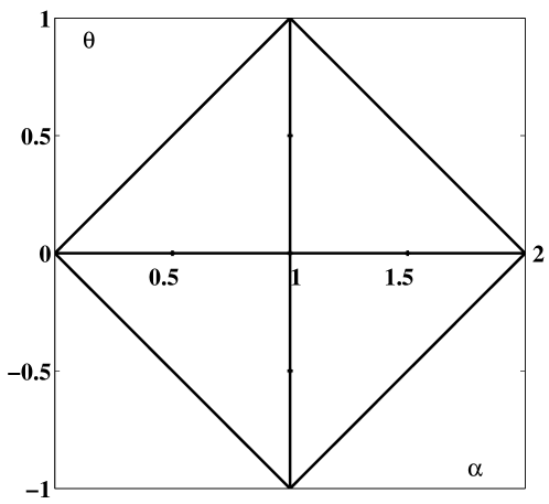
We note that the allowed region for the parameters $\alpha$ and $\theta$ turns out to be a diamond in the plane $\{\alpha\,,\,\theta\}$ with vertices in the points $(0,0)\,,\,(1,1)\,,\,(2,0)\,,\,(1,-1)\,,$ that we call the Feller-Takayasu diamond, see Fig. 1.

For $\alpha=2$ (henceforth $\theta=0$) we have $\widehat{\,{}_{x}D_{0}^{2}}(\kappa)=-\kappa^{2}=(-i\kappa)^{2}\,,$ so we recover the standard second derivative. More generally for $\theta=0$ we have $\widehat{\,{}_{x}D_{0}^{\alpha}}(\kappa)=-|\kappa|^{\alpha}=-(\kappa^{2})^{\alpha/2}$ so

$$\,{}_{x}D_{0}^{\alpha}=-\left(-{d^{2}\over dx^{2}}\right)^{\alpha/2}\,.$$

In this case we refer to the LHS of (2.5) as simply to the Riesz fractional derivative of order $\alpha\,.$ We refer to the Appendix A for the explicit expression of the generic Riesz-Feller derivative.

Let us now consider the Caputo fractional derivative in time. Following the original idea by Caputo [3, 4], see also [7, 8], [22], [50], a proper time fractional derivative of order $\beta\in(0,1)\,,$ useful for physical applications, may be defined in terms of the following rule for the Laplace transform

$${\cal L}\left\{{}_{t}D_{*}^{\beta}\,f(t);s\right\}=s^{\beta}\,\widetilde{f}(s)-s^{\beta-1}\,f(0^{+})\,,\quad 0<\beta<1\,,$$

where $\widetilde{f}(s)={\cal L}\left\{f(t);s\right\}=\int_{0}^{\infty}\hbox{e}^{\displaystyle\,-st}\,f(t)\,dt\,.$ Then the Caputo fractional derivative of $f(t)$ turns out to be defined as

$${}_{t}D_{*}^{\beta}\,f(t):=\cases{{\displaystyle{1\over{\Gamma(1-\beta)}}}\,{\displaystyle\int_{0}^{t}{\displaystyle{f^{(1)}(\tau)\over(t-\tau)^{\beta}}\,d\tau}}\,,&$\;0<\beta<1\,,$\cr\cr{\displaystyle{df(t)\over dt}}\,,&$\;\beta=1\,.$\cr}$$

In other words the operator $\,{}_{t}D_{*}^{\beta}$ is required to generalize the well-known rule for the Laplace transform of the first derivative of a given (causal) function keeping the standard initial value of the function itself. We refer to the Appendix B for the relation of this derivative to the more common Riemann Liouville fractional integral and derivative. Here we report the most relevant formula (B.6) which provides alternative expressions for the Caputo fractional derivative for $0<\beta<1\,:$

$${}_{t}D_{*}^{\beta}\,f(t)=\cases{{\displaystyle{1\over{\Gamma(1-\beta)}}\,{d\over dt}}\,{\displaystyle\int_{0}^{t}{f(\tau)-f(0^{+})\over(t-\tau)^{\beta}}\,d\tau}\,,\cr\cr{\displaystyle{1\over{\Gamma(1-\beta)}}\,{d\over dt}}\,{\displaystyle\int_{0}^{t}{f(\tau)\over(t-\tau)^{\beta}}\,d\tau}-f(0^{+})\,{\displaystyle{t^{-\beta}\over\Gamma(1-\beta)}}\,.\cr}$$

It is worth to note that the time fractional derivative in the L.H.S. of Eq. (2.2) can be removed by a suitable fractional integration, see (B.4), leading to the alternative form

$$u(x,t)=u(x,0^{+})+{\displaystyle{1\over\Gamma(\beta)}}\,{\displaystyle\int_{0}^{t}}{\,{}_{x}D^{\alpha}_{\theta}}\,u(x,\tau)\ \,{d\tau\over(t-\tau)^{1-\beta}}\,.$$

Differentiating with respect to time we have another equivalent form

$${\partial\over\partial t}\,u(x,t)={\displaystyle{1\over\Gamma(\beta)}}\,{\partial\over\partial t}\,\left\{{\displaystyle\int_{0}^{t}}{\,{}_{x}D^{\alpha}_{\theta}}\,u(x,\tau)\,{d\tau\over(t-\tau)^{1-\beta}}\right\}\,.$$

It is well known that in the case of standard diffusion Eq (2.1) can be derived from the continuity equation,

$${\partial\over\partial t}\,u(x,t)+{\displaystyle{\partial\over\partial x}}\,F\left[u(x,t)\right]=0\,,$$

where $F$ is the flux given by

$$F\left[u(x,t)\right]=-{\displaystyle{\partial\over\partial x}}\,u(x,t)\,.$$

Whereas Eq. (2.11) is related to a conservation law of a physical quantity (therefore it has a universal character), Eq. (2.12) is a phenomenological law which states that the flux is proportional to the gradient of the field variable (the transported quantity) with opposite sign. It is met in several physical contexts with different names: e.g. when $u$ is the temperature it is known as Fourier’s law, when $u$ is the pore pressure as Darcy’s law, when $u$ is a concentration of particles, as Fick’s law. Here we use the last terminology in view of the possible applications in chemical physics. We recall that Fick’s law is essentially an empirical law, which represents the simplest (local in space and time) relationship between the flux $F$ and the gradient of the concentration $u$ observable in several physical phenomena. As a matter of fact, for some experimental evidences in complex transport phenomena, this law can be replaced by a more suitable phenomenological relationship which may account for possible non-local and memory effects, without violating the conservation law expressed by the continuity equation (2.11). Now it is not difficult to derive our fractional diffusion equation in the form (2.10) from a generalized Fick’s law in which a suitable space-time operator depending on $\alpha,\theta$ and $\beta$ is acting on the gradient. After simple manipulations based on recent results by Paradisi et al [48, 49] and Gorenflo et al [26], we can write

$$F(x,t)=\,_{t}D^{1-\beta}\;_{x}P_{\theta}^{\alpha}\,\left[-{\partial\over\partial x}\,u(x,t)\right]\,,$$

where $\,{}_{t}D^{1-\beta}$ denotes the Riemann-Liouville fractional derivative of order $1-\beta$ (in time), see (B.1), and $\,{}_{x}P_{\theta}^{\alpha}$ is the pseudo-differential operator with symbol

$$\widehat{\,{}_{x}P_{\theta}^{\alpha}}(\kappa):={\widehat{\,{}_{x}D_{\theta}^{\alpha}}(\kappa)\over\widehat{\,{}_{x}D^{2}}(\kappa)}=|\kappa|^{\displaystyle\,\alpha-2}\,\hbox{e}^{\,\displaystyle i(\hbox{sign}\,\kappa)\theta\pi/2}\,.$$

For $\alpha=2$ and $\beta=1$ we recover the standard Fick’s law since in this case $\,{}_{t}D^{0}\,\,_{x}P^{2}_{0}=I$ (Identity). For $1<\alpha<2\,$ Eq. (2.13) results to be a a non-local connection between the flux and the concentration gradient both from temporal and spatial view points. For the nature of the operators involved, Eq. (2.13) can be referred to as the fractional Fick’s law: it turns out to be consistent with the space-time fractional diffusion equation (2.2). We note that for $0<\alpha\leq 1\,$ Eq. (2.13) is meaningless since the symbol of the pseudo-differential $P^{\alpha}_{\theta}$ in (2.14) exhibits at $\kappa=0$ a singularity not Fourier integrable, which means that the kernel is not integrable in $\bf{R}$. Generalized Fick’s laws with fractional derivatives have also been considered by other authors, including e.g. Zanette [65] and Caputo [5, 6].

3 The Green function for the space-time fractional diffusion

The fundamental solution (or the Green function) for the space-time fractional diffusion is intended to be the solution of the governing equation (2.2), or (2.9) or (2.10), corresponding to the initial condition $u(x,0^{+})=\delta(x)\,,$ It will be denoted by ${G_{\alpha,\beta}^{\theta}}(x,t)\,.$ In the case of standard diffusion, see Eq. (2.1), the Green function is nothing but the Gaussian probability density function with variance $\sigma^{2}=2t\,,$ namely

$$G_{2,1}^{0}(x,t)={1\over 2\sqrt{\pi}}\,t^{-1/2}\,\hbox{e}^{-\displaystyle x^{2}/(4t)}\,.$$

In the general case, following the arguments by Mainardi, Luchko & Pagnini [37] we can prove that ${G_{\alpha,\beta}^{\theta}}(x,t)$ is still a probability density evolving in time with the noteworthy scaling property

$${G_{\alpha,\beta}^{\theta}}(x,t)=t^{-\beta/\alpha}\,K_{\alpha,\beta}^{\theta}\left(x/t^{\beta/\alpha}\right)\,.$$

Here $x/t^{\beta/\alpha}\,$ acts as the similarity variable and $K_{\alpha,\beta}^{\theta}(\cdot)$ as the reduced Green function. For the analytical and computational determination of the reduced Green function, from now on we restrict our attention to $x>0\,$ because of the symmetry relation $K_{\alpha,\beta}^{\theta}(-x)=K_{\alpha,\beta}^{-\theta}(x)\,.$ Mainardi, Luchko & Pagnini [37] have provided (for $x>0$) the Mellin-Barnes integral representation

$$K_{\alpha,\beta}^{\theta}(x)={1\over\alpha x}{1\over 2\pi i}\int_{\gamma-i\infty}^{\gamma+i\infty}{\Gamma({s\over\alpha})\,\Gamma(1-{s\over\alpha})\,\Gamma(1-s)\over\Gamma(1-{\beta\over\alpha}s)\,\Gamma(\rho\,s)\,\Gamma(1-\rho\,s)}\,x^{\,\displaystyle s}\,ds\,,\;\rho={\alpha-\theta\over 2\,\alpha}\,,$$

where $0<\gamma<\hbox{min}\{\alpha,1\}\,.$

We recognize from the footnote ⁷ that Eq. (3.3) by changing $s$ into $-s$ can be interpreted as a Mellin transform pair that allows us to write the Mellin transform of $x\,K_{\alpha,\beta}^{\theta}(x)$ as

$$\quad\quad\quad\quad\quad\int_{0}^{+\infty}\!\!K_{\alpha,\beta}^{\theta}(x)\,x^{\,\displaystyle s}\,dx={1\over{\alpha}}\,{\Gamma(-{s/\alpha})\,\Gamma(1+{s/\alpha})\,\Gamma(1+s)\over\Gamma(1+{\beta s/\alpha})\,\Gamma(-\rho\,s)\,\Gamma(1+\rho\,s)}\,,\quad\quad\quad\quad$$

$$-\hbox{min}\{\alpha,1\}<\Re(s)<0\,.$$

In order to include $s=0$ in the convergence strip (so, in particular, the integral of $K_{\alpha,\beta}^{\theta}(x)$ in $\bf{R}_{0}^{+}$ can be evaluated) we properly use in (3.4) the functional equation $\Gamma(1+z)=z\,\Gamma(z)$ to obtain

$$\quad\quad\quad\quad\quad\int_{0}^{+\infty}\!\!K_{\alpha,\beta}^{\theta}(x)\,x^{\,\displaystyle s}\,dx=\rho\,{\Gamma(1-{s/\alpha})\,\Gamma(1+{s/\alpha})\,\Gamma(1+s)\over\Gamma(1-\rho\,s)\,\Gamma(1+\rho\,s)\,\Gamma(1+{\beta\,s/\alpha})}\,,\quad\quad\quad\quad\quad$$

$$-\hbox{min}\{\alpha,1\}<\Re(s)<\alpha\,.$$

In particular we find $\int_{0}^{+\infty}K_{\alpha,\beta}^{\theta}(x)\,dx=\rho\,$ (with $\rho=1/2$ if $\theta=0$).

We note that Eq. (3.5) is strictly valid as soon as cancellations in the ”gamma fraction” at the RHS are not possible. Then this equation allows us to evaluate (in $\bf{R}_{0}^{+}$) the (absolute) moments of order $\delta$ for the Green function such that $-\hbox{min}\{\alpha,1\}<\delta<\alpha\,.$ In other words, it states that $\,K_{\alpha,\beta}^{\theta}(x)={\cal O}\left(x^{-(\alpha+1)}\right)$ as $x\to+\infty\,.$ When cancellations occur in the ”gamma fraction” the range of $\delta$ may change. An interesting case is $\,\{\alpha=2,\,\theta=0,\,0<\beta\leq 1\}$ (time-fractional diffusion including standard diffusion), where Eq. (3.5) reduces to

$$\int_{0}^{+\infty}\!\!K_{2,\beta}^{0}(x)\,x^{\,\displaystyle s}\,dx={1\over{2}}\,{\Gamma(1+s)\over\Gamma(1+{\beta\,s/2})}\,,\quad\Re(s)>-1\,.$$

This result proves the existence of all moments of order $\delta>-1$ for the corresponding Green function. In virtue of (3.2), (3.6) we have

$$\int_{-\infty}^{+\infty}\!\!\!|x|^{\displaystyle\,\delta}\,G_{2,\beta}^{0}(x,t)\,dx={\Gamma(\delta+1)\over\Gamma(\beta\,\delta/2+1)}\,t^{\displaystyle\,\beta\,\delta/2}\,,\quad\delta>-1\,,\quad 0<\beta\leq 1\,,$$

and, for $\delta=2\,,$ the following formula for the variance

$$\int_{-\infty}^{+\infty}\!\!\!x^{\displaystyle\,2}\,G_{2,\beta}^{0}(x,t)\,dx={2\over\Gamma(\beta+1)}\,t^{\displaystyle\,\beta}\,,\quad 0<\beta\leq 1\,.$$

We note that the Mellin-Barnes integral representation allows us to construct computationally the fundamental solutions of Eq. (2.1) for any triplet $\{\alpha,\beta,\theta\}$ by matching their convergent and asymptotic expansions, see [37], [47]. Readers acquainted with Fox $H$ functions can recognize in (3.3) the representation of a certain function of this class, see e.g. [29], [39], [40], [53], [56], [57] [58], [62]. Unfortunately, as far as we know, computing routines for this general class of special functions are not yet available.

Let us now point out the main characteristics of the peculiar cases of strictly space fractional diffusion, strictly time fractional diffusion, and neutral fractional diffusion based on the results stated in [37].

For $\beta=1$ and $0<\alpha<2$ (strictly space fractional diffusion) we recover the class of the strictly stable (non-Gaussian) densities exhibiting heavy tails (with the algebraic decay $\propto|x|^{-(\alpha+1)}$) and infinite variance. For $\alpha=2$ and $0<\beta<1$ (strictly time fractional diffusion) we recover the class of the Wright-type densities exhibiting stretched exponential tails and finite variance proportional to $t^{\beta}\,.$ Mathematical details on these two classes of probability densities can be found in [37]; for further reading we refer to Schneider [56] for stable densities, and to Gorenflo, Luchko & Mainardi [20, 21] for the Wright-type densities.

As for the stochastic processes governed by these distributions we can expect the following.

For the case of non-Gaussian stable densities we expect a special class of Markovian processes, called stable Lévy motions, which exhibit infinite variance associated to the possibility of arbitrarily large jumps (Lévy flights), whereas for the case of Wright-type densities we expect a class of stochastic non-Markovian processes, which exhibit a (finite) variance consistent with slow anomalous diffusion.

For the special case $\alpha=\beta\leq 1$ (neutral diffusion) we obtain from (3.3) an elementary (non-negative) expression

$$\qquad\qquad\qquad K_{\alpha,\alpha}^{\theta}(x)={1\over\alpha x}{1\over 2\pi i}\int_{\gamma-i\infty}^{\gamma+i\infty}{\Gamma({s\over\alpha})\,\Gamma(1-{s\over\alpha})\over\Gamma(\rho\,s)\,\Gamma(1-\rho\,s)}\,x^{\,\displaystyle s}\,ds\qquad\qquad\qquad$$

$$={1\over\alpha x}{1\over 2\pi i}\int_{\gamma-i\infty}^{\gamma+i\infty}{\sin(\pi\,\rho\,s)\over\sin(\pi\,s/\alpha)}\,x^{\,\displaystyle s}\,ds={{1\over\pi}}\,{x^{\alpha-1}\sin[{\pi\over 2}(\alpha-\theta)]\over 1+2x^{\alpha}\cos[{\pi\over 2}(\alpha-\theta)]+x^{2\alpha}}\,,\quad x>0\,,$$

where $0<\gamma<\alpha\,.$

For the generic case of strictly space-time diffusion ($0<\alpha<2,\,0<\beta<1$), including neutral diffusion for $\alpha=\beta<1$, Mainardi, Luchko & Pagnini [37] have proven the non negativity of the corresponding reduced Green function and consequently its interpretation as probability density. In this case we obtain a class of probability densities (symmetric or non-symmetric according to $\theta=0$ or $\theta\neq 0$) which exhibit heavy tails with an algebraic decay $\propto|x|^{-(\alpha+1)}\,.$ Thus they belong to the domain of attraction of the Lévy stable densities of index $\alpha$ and can be referred to as fractional stable densities, according to a terminology proposed by Uchaikin [60]. The related stochastic processes are expected to possess the characteristics of the previous two classes. Indeed, they are non-Markovian (being $\beta<1$) and exhibit infinite variance associated to the possibility of arbitrarily large jumps (being $\alpha<2$).

4 The discrete random walk models for the Markovian fractional diffusion

It is known that a numerical approach to the standard diffusion equation (2.1) based on a proper finite difference scheme provides a discrete Markovian random walk model for the classical Brownian motion, see e.g. Zauderer [66].

In this section we intend to generalize this approach (that will be hereafter recalled) in order to provide a discrete Markovian random walk model for the Lévy stable motion of any order $\alpha\in(0,2)$ and skewness $\theta$ restricted as in (2.3). For this purpose we present a notable finite-difference approach to the strictly space fractional diffusion equation subjected to relevant restrictions, as we shall show in the following.

The common starting point of our analysis is obviously the discretization of the space-time domain by grid points and time instants as follows

$$\cases{x_{j}=j\,h\,,\quad h>0\,,\quad j=0,\pm 1,\pm 2,\dots\,;\cr t_{n}=n\,\tau\,,\quad\tau>0\,,\quad n=0,1,2,\dots\cr}$$

where the steps $h$ and $\tau$ are assumed to be small enough. The dependent variable $u$ is then discretized by introducing $y_{j}(t_{n})$ as

$$y_{j}(t_{n})\approx\int_{x_{j}-h/2}^{x_{j}+h/2}\!\!\!u(x,t_{n})\,dx\approx h\,u(x_{j},t_{n})\,.$$

4.1 The discrete random walk model for the standard diffusion

Let us now consider the standard diffusion equation (2.1). With the quantities $y_{j}(t_{n})$ so intended, we replace Eq. (2.1), after multiplication by the spatial mesh-width $h$, by the finite-difference equation

$${y_{j}(t_{n+1})-y_{j}(t_{n})\over\tau}={y_{j+1}(t_{n})-2y_{j}(t_{n})+y_{j-1}(t_{n})\over h^{2}}\,.$$

accepting that for positive $n$ in (4.3) we have approximate instead of exact equality. Since we are interested to approximate the fundamental solution (the Green function), we must equip (4.3) with the initial condition $y_{j}(0)=\delta_{j\,0}\,,$ where the Kronecker symbol represents the discrete counterpart of the Dirac delta function.

This approach can be interpreted as a discrete (in space and time) redistribution process of some extensive quantity provided it is conservative. If the extensive quantity is non-negative, e.g. mass or a sojourn probability, we have to preserve its non-negativity. In the first case the $y_{j}(t_{n})$ are imagined as clumps of mass, sitting at grid points $x=x_{j}$ in instants $t=t_{n}\,,$ which collect approximatively the total mass in the interval $x_{j}-h/2<x\leq x_{j}+h/2\,.$ In the second case, the $y_{j}(t_{n})$ may be interpreted as the probability of sojourn in point $x_{j}$ at time $t_{n}\,$ for a particle making a random walk on the spatial grid in discrete instants. From now on, we agree to pursue the probabilistic point of view.

In order to have a conservative and non-negativity preserving redistribution process, the discrete variable $y_{j}$ is subjected to the conditions

$$\sum_{j=-\infty}^{+\infty}y_{j}(t_{n})=\sum_{j=-\infty}^{+\infty}y_{j}(0)\,,\quad y_{j}(t_{n})\geq 0\,,\quad\hbox{for}\;\;\hbox{all}\;j\in\bf{Z}\,,\;n\in\bf{N}_{0}\,.$$

We easily recognize that our discrete redistribution process is akin to a Markov chain: when time proceeds from $t=t_{n}$ to $t=t_{n+1}\,,$ the sojourn-probabilities are redistributed according to the transition law

$$y_{j}(t_{n+1})=\sum_{k=-\infty}^{\infty}\,p_{k}\,y_{j-k}(t_{n})\,,\quad j\in\bf{Z}\,,\quad n\in\bf{N}_{0}\,,$$

where the $p_{k}$ denote suitable transfer coefficients, which represent the probability of transition from $x_{j-k}$ to $x_{j}$ (likewise from $x_{j}$ to $x_{j+k}$). The transfer coefficients are to be found consistently with the finite-difference equation (4.3) equipped with the proper initial condition. The process turns out to be both spatially homogeneous (the probability $p_{k}$ of jumping from a point $x_{j}$ to a point $x_{j+k}$ not depending on $j$) and time-stationary (the $p_{k}$ not depending on $n$), as is advised when considering our Cauchy problem and the definition of the difference operators. Furthermore the transfer coefficients must satisfy the conditions

$$\sum_{k=-\infty}^{\infty}p_{k}=1\,,\quad p_{k}\geq 0\,,\quad k=0\,,\,\pm 1\,,\,\pm 2\,,\,\dots$$

The transfer coefficients in our special case are easily deduced from (4.3) and (4.5): they turn out to be

$$p_{0}=1-2{\tau\over h^{2}}\,,\quad p_{\pm 1}={\tau\over h^{2}}\,,\quad p_{\pm k}=0\,,\quad k=2,3\dots\,,.$$

subject to the condition

$$0<\mu:={\tau\over h^{2}}\leq\mu_{max}={1\over{2}}\,.$$

We refer to Eqs (4.6)-(4.8) as the basic equations for the standard random walk model for the Gaussian process. The constant $\mu$ will be denoted as the scaling parameter of the standard diffusion equation. We recognize that only jumps of one step to the right or to the left or jumps of width zero occur. This corresponds to a well-known simple approximate realization of the Brownian motion.

The finite difference scheme (4.3) can be used for producing sample paths of individual particles performing the Brownian motion and for producing histograms of the approximate realization of the Gaussian density, by simulating many individual paths with the same number of time steps and making statistics of the final positions of the particles.

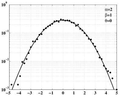
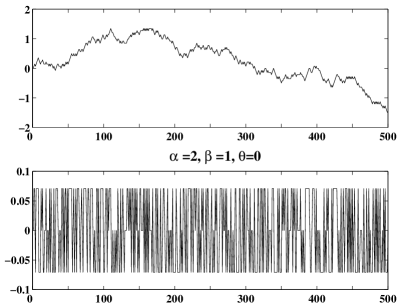
Our simulations, based on 10,000 realizations, have been limited to the interval $|x|\leq 5\,,$ where we have considered the random walks to take place, have produced an histogram for the Gaussian density at $t=1\,,$ see Fig 2 (left plate). Then, particles leaving this space have been ignored. In Fig 2 (right plate) we have displayed a particular sample path or trajectory (up) and the corresponding increment series (below) obtained with $N=500$ time steps, by taking an intermediate value for the scaling factor ($\mu=0.4<1/2$) and reasonable values for the space and time steps ($h=0.0707\,,$ $\,\tau=0.002$) in order to get $N\tau=t=1\,.$ Of course the histogram has been depicted by adopting a space step much larger than for the sample path, namely $h=0.25\,.$

Figure 2: Histogram (left) and a sample path with increments (right) for standard diffusion $\{\alpha=2\,,\;\beta=1\,,\;\theta=0\}$ (Brownian motion)

4.2 A discrete random walk model for the strictly space fractional diffusion

Discretizing all the variables as done for the standard diffusion equation, namely introducing a space-time mesh of widths $h$ and $\tau$ and a discrete variable $y_{j}(t_{n})$ interpreted as in (4.2), the essential idea is to replace the strictly space fractional diffusion equation by the finite-difference equation

$${y_{j}(t_{n+1})-y_{j}(t_{n})\over\tau}\,=\,_{h}D_{\theta}^{\alpha}\,y_{j}(t_{n})\,,\quad 0<\alpha<2\,,|\theta|\leq\,\hbox{min}\,\{\alpha,2-\alpha\}\,,$$

where the difference operator ${}_{h}D_{\theta}^{\alpha}$ is intended to converge to $D_{\theta}^{\alpha}$ (discussed in Appendix A) as $h\to 0\,.$ As usual, we have adopted a forward difference quotient in time at level $t=t_{n}$ for approximating the first-order time derivative. For ${}_{h}D_{\theta}^{\alpha}$ we require a scheme which must reduce as $\alpha=2$ to a symmetric second-order difference quotient in space at level $t=t_{n}\,,$ which has been adopted for approximating the second-order space derivative. Furthermore, the the finite-difference equation (4.9) is required to be consistent with a conservative, non-negativity preserving redistribution process, subject to the initial condition $y_{j}(0)=\delta_{j\,0}\,.$ Referring to Eqs (A.4), (A.8) and (A.10)-(A.11), we write

$${}_{h}D_{\theta}^{\alpha}\,y_{j}(t_{n})=\cases{-\,\left[c_{+}(\alpha,\theta)\,_{h}D^{\alpha}_{+}+c_{-}(\alpha,\theta)\,_{h}D^{\alpha}_{-}\right]\,y_{j}(t_{n})\,,&$\alpha\neq 1\,,$\cr\cr\left[\cos(\theta\pi/2)\,_{h}D_{0}^{1}+\,\sin(\theta\pi/2)\,_{h}D_{\pm}\right]\,y_{j}(t_{n})\,,&$\alpha=1\,.$\cr}$$

With the notation $\,{}_{h}D_{\pm}$ we intend to adopt $\,{}_{h}D_{+}$ when $0<\theta\leq 1$ and $\,{}_{h}D_{-}$ when $-1\leq\theta<0\,.$

We thus must find suitable finite-difference schemes for the pseudo-differential operators entering the Feller derivative, namely ${}_{h}D_{\pm}^{\alpha}$ (Weyl fractional derivatives of order $\alpha$) if $\alpha\neq 1$ and ${}_{h}D_{0}^{1}$ (Riesz derivative of first-order) if $\alpha=1\,.$ For this purpose we must keep distinct the three cases

$$\cases{\hbox{(a)}\quad 0<\alpha<1\,,&$|\theta|\leq\alpha\,;$\cr\hbox{(b)}\quad 1<\alpha<2\,,&$|\theta|\leq 2-\alpha\,;$\cr\hbox{(c)}\quad\alpha=1\,,&$|\theta|\leq 1\,.$\cr}$$

For $\alpha\neq 1$ the starting point is the Grünwald-Letnikov discretization of fractional derivatives, on which the reader can inform himself from the treatises on fractional calculus, see e.g. [42], [46], [50], [53], or in the review article by Gorenflo [18]. However, for our purposes, we must make a clever use of the Grünwald-Letnikov scheme treating separately the two cases (a) and (b) in order to be consistent with a conservative, non-negativity preserving redistribution process. We have

$${}_{h}D_{\pm}^{\alpha}\,y_{j}=\cases{{\displaystyle{\!1\over h^{\alpha}}}\,\sum\limits_{k=0}^{\infty}(-1)^{k}{\displaystyle\left({\alpha\atop k}\right)}\,y_{j\mp k}\,,&in the case (a) $0<\alpha<1\,,$\cr{\displaystyle{\!1\over h^{\alpha}}}\,\sum\limits_{k=0}^{\infty}(-1)^{k}{\displaystyle\left({\alpha\atop k}\right)}\,y_{j\pm 1\mp k}\,,&in the case (b) $1<\alpha<2\,.$\cr}$$

Notice the shift of index in the case (b) which among other things has the effect that in the limiting case $\alpha=2$ (the classical diffusion equation) we obtain the standard symmetric three-point difference scheme. For more details and discussions see Gorenflo & Mainardi [23].

For $\alpha=1$ we limit ourselves to consider the case $\theta=0$, that requires the discretization of the Hilbert transform in (A.11). The hyper-singular integral representation of the symmetric space-fractional derivative (the ”Riesz derivative”) given by Gorenflo & Mainardi in [25] [as formula (2.20)] readily offers us the discretization

$${}_{h}D_{0}^{1}y_{j}={1\over\pi\,h}\,\sum_{k=1}^{\infty}{y_{j+k}-2y_{j}+y_{j-k}\over k(k+1)}\,.$$

For $0<|\theta|\leq 1$ we have analogously to (A.10) to take into account the forward/backward difference quotients for $\,{}_{h}D_{\pm}$

$${}_{h}D_{+}={y_{j+1}-y_{j}\over h}\,,\quad_{h}D_{-}={y_{j}-y_{j-1}\over h}\,,$$

to obtain a non-negative scheme in a proper way. However, we here leave out these ”drifts” (in negative or positive directions) from the computation of the transfer coefficients $p_{k}$.

Then, inserting the expressions (4.12)-(4.13) in the finite-difference equation (4.9)-(4.10) yields the transition law

$$y_{j}(t_{n+1})=\sum_{k=-\infty}^{\infty}\,p_{k}\,y_{j-k}(t_{n})\,,\quad j\in\bf{Z}\,,\quad n\in\bf{N}_{0}\,,$$

where the transfer coefficients $p_{k}$ turn out to be, respectively,

$$\cases{p_{0}=1-\mu\,(c_{+}+c_{-})=1-\mu\,{\displaystyle{\cos\,(\theta\pi/2)\over\cos\,(\alpha\pi/2)}}\,,\cr p_{\pm k}=(-1)^{k+1}\mu\,{\displaystyle{\alpha\choose k}}\,c_{\pm}\,,\quad k=1,2,\dots\cr}\quad 0<\alpha<1\,,\;|\theta|\leq\alpha\,;$$

$$\cases{p_{0}=1+\mu\,{\displaystyle{\alpha\choose 1}}\,(c_{+}+c_{-})=1-\mu\,\alpha\,{\displaystyle{\cos\,(\theta\pi/2)\over|\cos\,(\alpha\pi/2)|}}\,,\cr p_{\pm 1}=-\mu\,\left[{\displaystyle{\alpha\choose 2}}\,c_{\pm}+c_{\mp}\right]\,,\qquad 1<\alpha<2\,,\;|\theta|\leq 2-\alpha\,;\cr p_{\pm k}=(-1)^{k}\,\mu\,{\displaystyle{\alpha\choose k+1}}\,c_{\pm}\,,\quad k=2,3,\dots\cr}$$

$$\cases{p_{0}=1-{\displaystyle{2\mu\over\pi}}\,,\cr p_{\pm k}={\displaystyle{\mu\over\pi}}\,{\displaystyle{1\over k(k+1)}}\,,\quad k=1,2,\dots\,,\cr}\quad\alpha=1\,,\;\theta=0\,;$$

with the scale parameter

$$\mu:={\tau\over h^{\alpha}}\,,\quad 0<\alpha<2\,.$$

It is straightforward to check in all cases the summation condition ${\displaystyle\sum_{k=-\infty}^{\infty}p_{k}=1\,.}$ Since all $p_{\pm k}\geq 0\,,\;k\neq 0\,$ the non-negativity condition is met if we require $p_{0}\geq 0$, i.e. if the scale parameter $\mu$ is restricted as follows

$$0<\mu:={\tau\over h^{\alpha}}\leq\mu_{max}=\cases{{\displaystyle{\cos{\alpha\pi/2}\over\cos{\theta\pi/2}}},&$\;0<\alpha<1\,,\;|\theta|\leq\alpha\,,$\cr{\displaystyle{1\over\alpha}{|\cos{\alpha\pi/2}|\over\cos{\theta\pi/2}}},&$\;1<\alpha<2\,,\;|\theta|\leq 2-\alpha\,,$\cr{\displaystyle{\pi\over 2}},&$\;\alpha=1\,,\;\theta=0\,.$\cr}$$

We note that in both the limits $\alpha\to 1^{-}$ and $\alpha\to 1^{+}$ the permissible range of the scaling factor $\mu$ is vanishing. In numerical practice the consequence will be that if $\alpha$ is near 1 the convergence is slow: for good approximation we will need a very small step-time $\tau$ with respect to the step-length $h$.

Figure 3: Sketch of the transition scheme for the space-fractional random walker

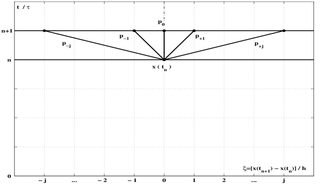
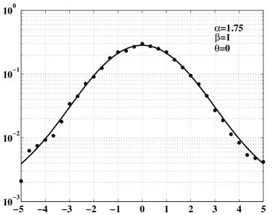
The striking difference to our discretized Brownian is the appearance of arbitrarily large jumps with power-like decay probability for which these discrete models are referred to as Lévy flights. See Fig. 3 for a sketch of the transition scheme and Section 6 for the numerical results.

5 The discrete random walk models for the non-Markovian fractional diffusion

Let us now try to generalize the above arguments by adapting them to the non-Markovian cases of our space-time fractional diffusion equation (2.2). We find it convenient to proceed by steps: we first consider the case of the strictly time fractional diffusion, see also [26], and then, by combining these arguments with those for strictly space fractional diffusion, we treat the strictly space-time fractional diffusion.

5.1 A discrete random walk model for the strictly time fractional diffusion

Discretizing all the variables as for the standard diffusion equation, namely introducing a space-time mesh of widths $h$ and $\tau$ and a discrete variable $y_{j}(t_{n})$ interpreted as in (4.2), the essential idea is to replace the strictly time fractional diffusion equation by the finite-difference equation

$${}_{\tau}D_{*}^{\beta}\,y_{j}(t_{n+1})={y_{j+1}(t_{n})-2y_{j}(t_{n})+y_{j-1}(t_{n})\over h^{2}}\,,\quad 0<\beta<1\,,$$

where the difference operator ${}_{\tau}D_{*}^{\beta}$ is intended to converge to $D_{*}^{\beta}$ as $\tau\to 0\,.$

As usual, we have adopted a symmetric second-order difference quotient in space at level $t=t_{n}$ for approximating the second-order space derivative. For ${}_{\tau}D_{*}^{\beta}$ we require a scheme which must reduce as $\beta=1$ to a forward difference quotient in time at level $t=t_{n}\,,$ which is usually adopted for approximating the first-order time derivative. Then, for approximating the time fractional derivative (in Caputo’s sense), we adopt a backward Grünwald-Letnikov scheme in time (starting at level $t=t_{n+1}$) which reads

$${}_{\tau}D_{*}^{\beta}\,y_{j}(t_{n+1})=\sum_{k=0}^{n+1}(-1)^{k}\,{\beta\choose k}\,{y_{j}(t_{n+1-k})-y_{j}(0)\over\tau^{\beta}}\,,\quad 0<\beta<1\,.$$

Here the subtraction of $y_{j}(0)$ in each term of the sum reflects the subtraction of $f(0^{+})$ in formula (B.6) for the Caputo fractional derivative. Combining (5.1) and (5.2), introducing the scaling parameter

$$\mu:={\tau^{\beta}\over h^{2}}\,,\quad 0<\beta\leq 1\,,$$

and using the ”empty sum” convention $\displaystyle{\sum_{k=p}^{q}=0}$ if $q<p\,$ (here $p=1$ when $q=n=0\,$), we obtain for $n\geq 0$ ($t_{0}=0$):

$$\qquad y_{j}(t_{n+1})=y_{j}(t_{0})\,\sum_{k=0}^{n}(-1)^{k}\,{\beta\choose k}+\sum_{k=1}^{n}(-1)^{k+1}\,{\beta\choose k}\,y_{j}(t_{n+1-k})\qquad\qquad\qquad$$

$$+\mu\,\left[y_{j+1}(t_{n})-2y_{j}(t_{n})+y_{j-1}(t_{n})\right]\,.$$

Thus, (5.4) provides the universal transition law from $t_{n}$ to $t_{n+1}$ valid for all $n\geq 0\,.$ For convenience let us introduce the coefficients $c_{k}$, $b_{m}$

$$\cases{c_{k}=(-1)^{k+1}\,{\displaystyle{\beta\choose k}}=\left|{\displaystyle{\beta\choose k}}\right|\,,\quad k\geq 1\,,\cr b_{m}={\displaystyle\sum_{k=0}^{m}(-1)^{k}\,{\beta\choose k}}\,,\quad m\geq 0\,.\cr}$$

For $\beta=1$ (standard diffusion) we note that all these coefficients are vanishing except $b_{0}=c_{1}=1\,.$ For $0<\beta<1$ they possess the properties

$$\sum_{k=1}^{\infty}c_{k}=1\,,\quad 1>\beta=c_{1}>c_{2}>c_{3}>\,\dots\,\to 0\,,$$

$$\cases{b_{0}=1={\displaystyle\sum_{k=1}^{\infty}\,c_{k}}\,,\quad b_{m}=1-{\displaystyle\sum_{k=1}^{m}\,c_{k}}={\displaystyle\sum_{k=m+1}^{\infty}\,c_{k}\,,}\cr 1=b_{0}>b_{1}>b_{2}>b_{3}>\,\dots\,\to 0\,.\cr}$$

We thus observe that the $c_{k}$ and the $b_{m}$ form sequences of positive numbers, not greater than 1, decreasing strictly monotonically to zero. Thanks to the introduction of the above coefficients the universal transition law (5.4) can be written in the following noteworthy form

$$y_{j}(t_{n+1})=b_{n}\,y_{j}(t_{0})+\sum_{k=1}^{n}c_{k}\,y_{j}(t_{n+1-k})+\mu\left[y_{j+1}(t_{n})-2y_{j}(t_{n})+y_{j-1}(t_{n})\right],$$

with the empty sum convention convention if $n=0\,.$ In particular we get, for $n=0\,:$

$$y_{j}(t_{1})=(1-2\mu)\,y_{j}(t_{0})+\mu\,\left[y_{j+1}(t_{0})+y_{j-1}(t_{0})\right]\,;$$

for $n=1\,:$

$$y_{j}(t_{2})=b_{1}y_{j}(t_{0})+(c_{1}-2\mu)\,y_{j}(t_{1})+\mu\,\left[y_{j+1}(t_{1})+y_{j-1}(t_{1})\right]\,;$$

for $n\geq 2\,:$

$$\begin{array}[]{ll}{\displaystyle y_{j}(t_{n+1})}=&{\displaystyle b_{n}\,y_{j}(t_{0})+\sum_{k=2}^{n}c_{k}\,y_{j}(t_{n+1-k})}\\ &{\displaystyle+(c_{1}-2\mu)\,y_{j}(t_{n})+\mu\,\left[y_{j+1}(t_{n})+y_{j-1}(t_{n})\right]}\,.\end{array}$$

Observe that $c_{1}=\beta\,.$ The scheme (5.8) preserves non-negativity, if all coefficients are non-negative, hence if

$$0<\mu={\tau^{\beta}\over h^{2}}\leq{\beta\over 2}\,.$$

Furthermore it is conservative, as we shall prove by induction: i.e.

$${\displaystyle\sum_{j=-\infty}^{+\infty}}|y_{j}(t_{0})|<\infty\,\Longrightarrow\,{\displaystyle\sum_{j=-\infty}^{+\infty}}y_{j}(t_{n})={\displaystyle\sum_{j=-\infty}^{+\infty}}y_{j}(t_{0})\,,\quad n\in\bf{N}\,.$$

In fact, putting $S_{n}={\displaystyle\sum_{j=-\infty}^{+\infty}}y_{j}(t_{n})$ for $n\geq 0\,,$ then from (5.8) we get

$$S_{1}=(1-2\mu)\,\sum y_{j}(t_{0})+\mu\sum y_{j-1}(t_{0})+\mu\sum y_{j+1}(t_{0})=S_{0},,$$

and for $n\geq 1$ we find always from (5.8), assuming $S_{0}=S_{1}=\dots S_{n}$ already proved,

$$\begin{array}[]{ll}{\displaystyle S_{n+1}}&={\displaystyle b_{n}\,S_{0}+\sum_{k=2}^{n}c_{k}\,S_{n+1-k}+(\beta-2\mu+\mu+\mu)\,S_{n}}\\ &={\displaystyle\left(b_{n}+\sum_{k=1}^{n}c_{k}\right)\,S_{0}=S_{0}}\,,\end{array}$$

using $\beta=c_{1}\,.$ We have thus proved conservativity. Non-negativity preservation and conservativity mean that our scheme can be interpreted as a redistribution scheme of clumps $y_{j}(t_{n})\,.$ For orientation on such aspects and for examples let us quote the works by Gorenflo on conservative difference schemes for diffusion problems, see e.g. [16, 17].

The interpretation of our redistribution scheme is as follows: the clump $y_{j}(t_{n+1})$ arises as a weighted-memory average of the (previous) $n+1$ values $y_{j}(t_{m})\,,$ with $m=n\,,\,n-1\,,\dots\,,1\,,0\,,$ with positive weights

$$\beta=c_{1},\,c_{2}\,,\dots\,,c_{n}\,,\quad b_{n}=1-{\displaystyle\sum_{k=1}^{n}c_{k}}\,,$$

followed by subtraction of $2\mu\,y_{j}(t_{n})$, which is given in equal parts to the neighbouring points $x_{j-1}$ and $x_{j+1}\,$ but replaced by the contribution $\,\mu\,[y_{j+1}(t_{n})+y_{j-1}(t_{n})]\,$ from these neighbouring points. For random walk interpretation we consider the $y_{j}(t_{n})$ as probabilities of sojourn at point $x_{j}$ in instant $t_{n}\,$ requiring the normalization condition ${\displaystyle\sum_{j=-\infty}^{+\infty}y_{j}(t_{0})}=1\,.$

For $n=0$ Equation (5.8) means (by appropriate re-interpretation of the spatial index $j$): A particle sitting at $x_{j}$ in instant $t_{0}$ jumps, when $t$ proceeds from $t_{0}$ to $t_{1}\,,$ with probability $\mu$ to the neighbour point $x_{j+1}\,,$ with probability $\mu$ to the neighbour point $x_{j-1}\,,$ and with probability $1-2\mu$ it remains at $x_{j}\,.$ For $n\geq 1$ we write (5.8), using $\beta=c_{1}\,,$ as follows:

$$\begin{array}[]{ll}{\displaystyle y_{j}(t_{n+1})}=&{\displaystyle\left(1-\sum_{k=1}^{n}c_{k}\right)\,y_{j}(t_{0})+c_{n}\,y_{j}(t_{1})+c_{n-1}\,y_{j}(t_{2})+\dots+c_{2}\,y_{j}(t_{n-1})}\\ &{\displaystyle+(c_{1}-2\mu)\,y_{j}(t_{n})+\mu\,\left[y_{j+1}(t_{n})+y_{j-1}(t_{n})\right]}\,.\end{array}$$

Obviously, all coefficients (probabilities) are non negative, and their sum is 1. But what does it mean? Having a particle, sitting in $x_{j}$ at instant $t_{n}\,,$ where will we find it with which probability at instant $t_{n+1}?$ From (5.12) we conclude, by re-interpretation of the spatial index $j\,,$ considering the whole history of the particle, i.e. the particle path $\left\{x(t_{0})\,,\,x(t_{1})\,,\,x(t_{2})\,,\,\dots\,,\,x(t_{n})\right\},$ that if at instant $t_{n}$ it is in point $x_{j}\,,$ there is the contribution $c_{1}-2\mu$ to be again at $x_{j}$ at instant $t_{n+1}\,,$ the contribution $\mu$ to go to $x_{j-1}\,,$ the contribution $\mu$ to go to $x_{j+1}\,.$ But the sum of these contributions is $c_{1}=\beta\leq 1\,.$ So, excluding the case $\beta=1$ in which we recover the standard diffusion (Markovian process), for $\beta<1$ we have to consider the previous time levels (non-Markovian process). Then, from level $t_{n-1}$ we get the contribution $c_{2}$ for the probability of staying in $x_{j}$ also at time $t_{n+1}\,,$ from level $t_{n-2}$ we get the contribution $c_{3}$ for the probability of staying in $x_{j}$ at time $t_{n+1}\,,\dots\,,$ from level $t_{1}$ we get the contribution $c_{n}$ for the probability of staying in $x_{j}$ at time $t_{n+1}\,,$ and finally, from level $t_{0}=0$ we get the contribution $b_{n}$ for the probability of staying in $x_{j}$ at time $t_{n+1}\,.$ Thus, the whole history up to $t_{n}$ decides probabilistically where the particle will be at instant $t_{n+1}\,.$

Let us consider the problem of simulation of transition from time level $t_{n}$ to $t_{n+1}$: Assume the particle sitting in $x_{j}$ at instant $t_{n}\,.$ Generate a random number equidistributed in $0\leq\rho<1\,,$ and subdivide the interval $[0,1)$ as follows. From left to right beginning at zero we put adjacent intervals of length $c_{1},c_{2},\dots,c_{n},b_{n}$, for consistency left-closed, right-open. The sum of these is 1. We divide further the first interval (of length $c_{1}$) into sub-intervals of length $\mu,c_{1}-2\mu,\mu\,.$ Then we look into which of the above intervals the random number falls. If in first interval with length $c_{1}=\mu+(c_{1}-2\mu)+\mu$, then look in which subinterval, and correspondingly move the particle to $x_{j-1}\,,$ or leave it at $x_{j}$ or move to $x_{j+1}\,.$ If the random number falls into one of the intervals with length $c_{2}\,,\,c_{3}\,,\,\dots\,,c_{n}$ (i.e. $c_{k}$ with $2\leq k\leq n$), then move the particle back to its previous position $x(t_{n+1-k})$, which by chance could be identical with $x_{j}=x(t_{n})\,.$ If the random number falls into the rightmost interval with length $b_{n}$ then move the particle back to its initial position $x(t_{0})\,,$ for which we recommend $x(t_{0})=0\,,$ meaning $y_{j}(t_{0})=\delta_{j0}\,,$ in accordance with the initial condition $u(x,0)=\delta(x)$ for (2.2) with $\alpha=2\,,\,\theta=0\,.$

A sketch of the transition scheme for the random walker is reported in Figure 4. Besides the diffusive part $(\mu\,,\,c_{1}-2\mu\,,\,\mu)$ which lets the particle jump at most to neighbouring points, we have for $0<\beta<1$ the memory part which gives a tendency to return to former positions even if they are far away. Due to Equations (5.6)-(5.7), of course, the probability to return to a far away point gets smaller and smaller the larger the time lapse is from the instant when the particle was there.

Figure 4: Sketch of the transition scheme for the time-fractional random walker

5.2 A discrete random walk model for the strictly space-time fractional diffusion

By combining the approach of the preceding Subsections 3.2 and 4.1 we can construct a discrete random walk model for the strictly space-time fractional diffusion equation, namely for the case$\{0<\alpha<2\,,\,0<\beta<1\}\,.$ We replace in (2.2) the (Riesz-Feller) space-fractional derivative by (4.10) and the (Caputo) time-fractional derivative by (5.2). Solving then for the ”new” value $y_{j}(t_{n+1})$ we see that the scaling parameter $\mu=\tau^{\beta}/h^{\alpha}$ plays the essential role in obtaining a scheme with all transition coefficients non-negative. In fact, also here $\mu$ must be restricted to a suitable interval $(0,\mu_{max}]\,.$ In analogy to the case of the strictly time fractional diffusion the ”discrete” diffusion in space occurs only between the time-level $t_{n}$ and $t_{n+1}$ and the memory part of the process only straight-backwards in time. However, in contrast to the strictly time fractional diffusion, the discrete diffusion (or the random walker) can now go to any grid point in space, not only to immediate neighbouring grid points. We abstain from presenting here all the lengthy formulas that again need distinction between the three cases: (a) $0<\alpha<1\,,$ (b) $1<\alpha<2\,,$ and (c) $\alpha=1\,.$

6 Numerical results and concluding discussions

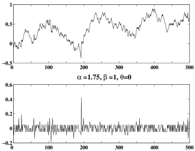
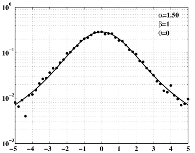
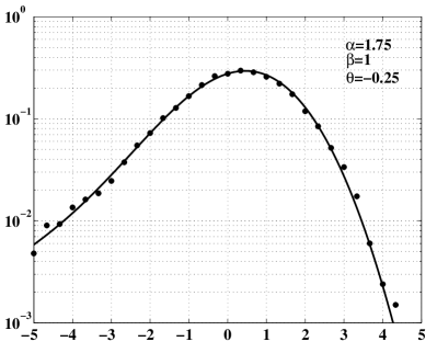
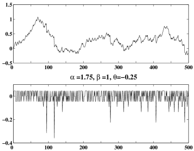
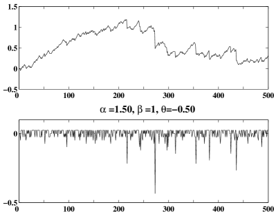
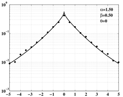
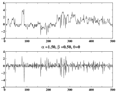
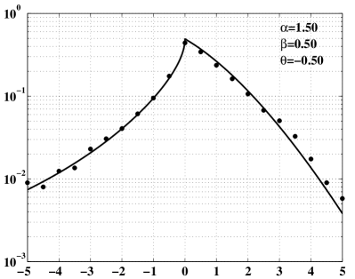
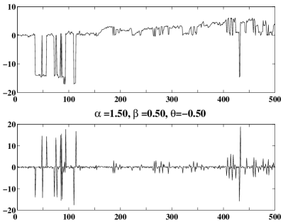
Our simulations are all based on 10,000 realizations. In addition to the Brownian motion, see Fig. 2, we have considered a set of 8 case-studies, see Figs 5-12, for our space-time fractional diffusion that, in our opinion, can better illustrate the state-of art of this analysis. The sample paths and the corresponding increments are plotted against the time steps up to 500, see the right figure-plates, while the histograms refer to densities at $t=1\,$ for $|x|\leq 5\,,$ see the left figure-plates. All the plots were drown by using the MATLAB system. The relevant parameters $\alpha$, $\theta$, $\beta$, $\mu$, $h$ and $\tau$ used in the Figures are reported in Table I. For convenience we have also reported the maximum value of the scaling parameter $\mu$ as can be deduced from our theoretical analysis. More details can be found in [45].

$\alpha$	$\theta$	$\beta$	$\mu_{max}$	$h_{S}$	$\tau_{S}$	$h_{H}$	$\tau_{H}$
$2$	$0$	$1$	$0.50$	$7.0\,10^{-2}$	$2.0\,10^{-3}$	$0.20$	$2.5\,10^{-2}$
$1.75$	$0$	$1$	$0.53$	$4.7\,10^{-2}$	$2.0\,10^{-3}$	$0.33$	$2.0\,10^{-2}$
$1.75$	$-.25$	$1$	$0.57$	$4.5\,10^{-2}$	$2.0\,10^{-3}$	$0.33$	$2.0\,10^{-2}$
$1.50$	$0$	$1$	$0.47$	$3.0\,10^{-2}$	$2.0\,10^{-3}$	$0.20$	$1.0\,10^{-2}$
$1.50$	$-.50$	$1$	$0.67$	$2.4\,10^{-2}$	$2.0\,10^{-3}$	$0.20$	$1.0\,10^{-2}$
$2$	$0$	$0.75$	$0.37$	$0.17$	$2.0\,10^{-3}$	$0.25$	$5.0\,10^{-3}$
$2$	$0$	$0.50$	$0.25$	$0.47$	$2.0\,10^{-3}$	$0.50$	$2.5\,10^{-2}$
$1.50$	$0$	$0.50$	$0.24$	$0.38$	$2.0\,10^{-3}$	$0.50$	$5.0\,10^{-3}$
$1.50$	$-.50$	$0.50$	$0.33$	$0.30$	$2.0\,10^{-3}$	$0.50$	$5.0\,10^{-3}$

Table I: The relevant parameters for the simulations

$\alpha$ = space-fractional order, $\,\theta$ = skewness, $\,\beta$ = time-fractional order,

$\mu=\tau^{\beta}/h^{\alpha}$ = scaling parameter,

$h_{S}$ = space-step, $\,\tau_{S}$ = time-step for sample paths,

$h_{H}$ = space-step, $\,\tau_{H}$ = time-step for histograms.

In practice, in our numerical studies there is required truncation for two different causes. As in the classical Brownian motion, a trivial truncation is required if a priori one wants a definite region of space to be considered in which the walk takes place. Then, particles leaving this space have been ignored. However, if $0<\alpha<2\,,$ at variance with our discretized Brownian motion, we now have an infinite number of transition probabilities. Since it is impossible to simulate all infinitely many discrete probabilities, so the size of possible jumps must be limited to a maximal possible jump length.

The plates in Fig. 5 are concerning two cases of symmetrical, strictly space fractional diffusion: $\{\alpha=1.75\,,\,\beta=1,\,\theta=0\}$, $\{\alpha=1.5\,,\,\beta=1,\,\theta=0\}$ whreas the plates in Fig. 6 are concerning two cases of extremal, strictly space fractional diffusion: $\{\alpha=1.75\,,\,\beta=1,\,\theta=-0.25\}$, $\{\alpha=1.5\,,\,\beta=1,\,\theta=-0.50\}$ From the sample paths in Figs. 5, 6 one can recognize the ”wild” character (with large jumps) of the Lévy flights with respect to the ”tame” character of the Brownian motion outlined in Fig. 2.

Figure 5: Histograms (left) and sample paths with increments (right) for symmetrical, strictly space fractional diffusion.

Figure 6: Histograms (left) and sample paths with increments (right) for extremal, strictly space fractional diffusion.

The plates in Fig. 7 are concerning two cases of strictly time fractional diffusion: $\{\alpha=2,\,\beta=0.75\}$ and $\{\alpha=2,\,\beta=0.50\}$; here the paths exhibit the memory effect visible in a kind of stickiness combined with occasional jumps to points previously occupied, in distinct contrast to the rather tame behaviour in case $\{\alpha=2,\,\beta=1\}$ (simulation of Brownian motion).

Figure 7: Histograms (left) and sample paths with increments (right) for strictly time fractional diffusion.

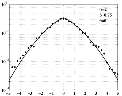
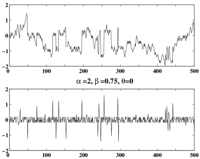
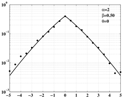
Finally, the plates in Fig. 8 are concerning two cases of strictly space-time fractional diffusion: $\{\alpha=1.50,\,\beta=0.50,\,\theta=0\}$ and $\{\alpha=1.50,\,\beta=0.50,\,\theta=-0.50\}$, where the combined effects of the previous cases are present.

We have used our discrete models for simulation of particle trajectories by interpreting our redistribution schemes as descriptions of Markov chains with infinitely many states, namely the possible positions $x_{j}$. However, as they have the form of difference schemes in a regular space-time grid they can ”in principle” also serve for the purpose of approximate computation of the temporal evolution of the density $u(x,t)$. Namely, we are expecting that $u(x_{j},t_{n})$ is approximated by $y_{j}(t_{n})/h$. In fact, from their essential properties (conservativity and preservation of non-negativity, see (4.6), (5.11) and (5.12) ) it can by standard methods of numerical analysis been shown that our models interpreted as difference schemes are stable and consistent, hence convergent. We say ”in principle” because for practical application appropriate truncations are required. That there is also convergence in the chain interpretation (complete convergence in the stochastic sense) can be shown by methods of Fourier and Laplace analysis, see Gorenflo and Mainardi in [24, 25] for the space fractional diffusion.

Figure 8: Histograms (left) and sample paths with increments (right) for strictly space-time fractional diffusion.

There are other methods of simulating space-fractional diffusion processes. Without attempting to be exhaustive, without going into details and without attempting to give a survey of the existing and growing literature on the subject let us mention a few possibilities: generations of random numbers distributed according to a given stable law, random walks discrete in time but continuous in space (namely jumps to arbitrary places in space, not only to grid points). Furthermore, let us mention here the Chechkin-Gonchar random walk (suggested and used in [9] and mathematically analyzed in [25]), and simulation via compound Poisson processes (with proper scaling of space and time), see [27].

In the special field of methods, discrete in space and time, there also are other methods available (see the methods sketched in [19] and discussed in detail in [24, 25] of which, in particular, the Gillis-Weiss random walk must be cited, see [14]). Final word: Still many questions are open in this challenging and fascinating field of research!

Appendix A: The Riesz-Feller space fractional derivatives

In this Appendix we provide the explicit expression of the Riesz-Feller fractional derivative $\,{}_{x}D^{\alpha}_{\theta}$ which, according to (2.4) is defined as the pseudo-differential operator with symbol

$$\widehat{\,{}_{x}D^{\alpha}_{\theta}}={\displaystyle-|\kappa|^{\alpha}}\,\hbox{e}^{\displaystyle i(\hbox{sign}\,\kappa)\theta\pi/2}\,.$$

Let us now express more properly the operator $\,-\,_{x}D_{\theta}^{\alpha}$ as inverse of a suitable integral operator $\,{}_{x}I_{\theta}^{\alpha}\,,$ whose symbol is required to be $\,{\displaystyle|\kappa|^{-\alpha}}\,\hbox{e}^{\displaystyle\,-i\,({\hbox{sign}\,}\,\kappa)\,\theta\pi/2}\,,$ so we may write

$${}_{x}D_{\theta}^{\alpha}:=-\,_{x}I_{\theta}^{-\alpha}\,.$$

This integral operator was found by Feller [12] in 1952 generalizing the approach by Marcel Riesz to Fractional Calculus, see e.g. [51], and it is referred to as Feller potential by Samko, Kilbas & Marichev [53]. Using our notation, the Feller potential reads

$$\,{}_{x}I_{\theta}^{\alpha}\,f(x)=c_{-}(\alpha,\theta)\,_{x}I_{+}^{\alpha}\,f(x)+c_{+}(\alpha,\theta)\,_{x}I_{-}^{\alpha}\,f(x)\,,$$

where, if $0<\alpha<2\,,\;\alpha\neq 1\,,$

$$c_{+}(\alpha,\theta)={\sin\,\left[(\alpha-\theta)\,\pi/2\right]\over\sin\,(\alpha\pi)}\,,\quad c_{-}(\alpha,\theta)={\sin\,\left[(\alpha+\theta)\,\pi/2\right]\over\sin(\alpha\pi)}\,,$$

and, by passing to the limit (with $\theta=0$) $c_{+}(2,0)=c_{-}(2,0)=-1/2\,.$ In (A.4) the operators $\,{}_{x}I_{\pm}^{\alpha}$ denote the Riemann-Liouville fractional integrals, also known as Weyl fractional integrals), defined as

$$\cases{{\,{}_{x}I_{+}^{\alpha}\,f(x)}={\displaystyle{1\over{\Gamma(\alpha)}}}\,{\displaystyle\int_{-\infty}^{x}\!\!(x-\xi)^{\alpha-1}\,f(\xi)\,d\xi}\,,\cr\cr{\,{}_{x}I_{-}^{\alpha}\,f(x)}={\displaystyle{1\over{\Gamma(\alpha)}}}\,{\displaystyle\int_{x}^{+\infty}\!\!(\xi-x)^{\alpha-1}\,f(\xi)\,d\xi}\,.\cr}$$

We note that whereas the coefficients $c_{\pm}$ can loose their meaning when $\alpha$ is an integer, the Riemann-Liouville integral operators $I_{\pm}^{\alpha}$ are well defined in their action on rapidly decreasing integrable functions, for any $\alpha\geq 0\,,$ being set equal to the identity operator when $\alpha=0\,,$ for convenience (justified by passage to the limit $\alpha\to 0$). In the particular case $\theta=0$ we get

$$c_{+}(\alpha,0)=c_{-}(\alpha,0)={1\over 2\,\cos\,(\pi\alpha/2)}\,,$$

and thus we recover the Riesz potential, see e.g. [53],

$$\,{}_{x}I_{0}^{\alpha}\,f(x):={1\over{2\,\Gamma(\alpha)\,\cos\,(\pi\alpha/2)}}\,\int_{-\infty}^{+\infty}\!\!\!|x-\xi|^{\alpha-1}\,f(\xi)\,d\xi\,.$$

The Riesz and the Feller potentials are well defined if the index is located in the interval $(0\,,\,1)\,,$ or in the interval $(0,2)\,,$ and we have the semigroup property, $\,{}_{x}I_{\theta}^{\alpha}\,\,{}_{x}I_{\theta}^{\beta}=\,_{x}I_{\theta}^{\alpha+\beta}\,,$ if $0<\alpha<1$, $0<\beta<1$ and $\alpha+\beta<1\,.$ Then, following Feller, we define by analytic continuation the pseudo-differential operator (A.2) in the whole range $0<\alpha\leq 2\,,\,\alpha\neq 1\,,$ as

$$\,{}_{x}D_{\theta}^{\alpha}:=-\left[c_{+}(\alpha,\theta)\,\,_{x}D_{+}^{\alpha}+c_{-}(\alpha,\theta)\,\,_{x}D_{-}^{\alpha}\right]\,,\quad 0<\alpha\leq 2\,.$$

where $\,{}_{x}D_{+}^{\alpha}:=\,_{x}I_{+}^{-\alpha}$ and $\,{}_{x}D_{-}^{\alpha}:=\,_{x}I_{-}^{-\alpha}$ are the inverses of the operators $\,{}_{x}I_{+}^{\alpha}$ and $\,{}_{x}I_{-}^{\alpha}\,,$ respectively, and are referred to as the Weyl fractional derivatives. When $\theta=0$ the Riesz-Feller derivative can be simply referred to as Riesz derivative. We note from (A.4) the property $\,c_{\pm}(\alpha,\theta)=c_{\mp}(-\alpha)\,.$ For integral representations of the operators $\,{}_{x}I_{\pm}^{-\alpha}$ see [53]; we have

$${}_{x}I_{\pm}^{-\alpha}=\cases{{\displaystyle\pm{d\over dx}}\,\left(\,{}_{x}I_{\pm}^{1-\alpha}\right)\,,&if $\quad 0<\alpha\leq 1\,,$\cr\cr{\displaystyle{d^{2}\over dx^{2}}}\,\left(\,{}_{x}I_{\pm}^{2-\alpha}\right)\,,&if $\quad 1<\alpha\leq 2\,.$\cr}$$

For $\alpha=2$ ($\theta=0$) we recover the standard second derivative. In fact, from (A.6) $c_{+}(2,0)=c_{-}(2,0)=-1/2\,,$ so from (A.8)-(A.9) ${}_{x}D_{0}^{2}=-I_{0}^{-2}=\left(\,{}_{x}I_{+}^{-2}+\,_{x}I_{-}^{-2}\right)/2=\left({d^{2}\over dx^{2}}+{d^{2}\over dx^{2}}\right)/2={d^{2}\over dx^{2}}=\,_{x}D^{2}\,.$ For $\alpha=1$ ($|\theta|\leq 1$) we have (from calculation with symbols)

$${}_{x}D^{1}_{\theta}\,f(x)=\left[\cos(\theta\pi/2)\,_{x}D_{0}^{1}+\sin(\theta\pi/2)\,_{x}D\right]\,f(x)\,,$$

where $\,{}_{x}D_{0}^{1}\,f(x)=-\,_{x}D\,\left[\,{}_{x}H\,f(x)\right]\,,$ with

$$\,{}_{x}H\,f(x)={1\over\pi}\,\int_{-\infty}^{+\infty}{f(\xi)\over x-\xi}\,d\xi={1\over\pi}\,\int_{-\infty}^{+\infty}{f(x-\xi)\over\xi}\,d\xi\,.$$

In (A.11) $\,{}_{x}H$ denotes the Hilbert transform (with symbol $\widehat{\,{}_{x}H}(\kappa)=i\,\hbox{sign}\,\,\kappa\,$) and its singular integral is understood in the Cauchy principal value sense. We note that in the limiting extremal cases $\theta=\pm 1$ we recover the standard first derivative, i.e. $\,{}_{x}D^{1}_{\pm 1}=\pm\,\,_{x}D\,.$

Appendix B: The Riemann-Liouville and Caputo time fractional derivatives

The purpose of this Appendix is to clarify for the interested reader the main differences between the Caputo fractional derivative $\,{}_{t}D_{*}^{\beta}$ adopted in this paper, see (2.8), and the Riemann-Liouville fractional derivative $\,{}_{t}D^{\beta}$ usually adopted in the literature. Any formula here is valid for $t>0\,,$ with the assumption that the function $f(t)$ has a finite limit as $t\to 0^{+}\,.$ We recall

$${}_{t}D^{\beta}\,f(t):=\cases{{\displaystyle{1\over{\Gamma(1-\beta)}}}\,{\displaystyle{d\over dt}}\,{\displaystyle\int_{0}^{t}{f(\tau)\over(t-\tau)^{\beta}}\,d\tau}\,,&$\;0<\beta<1\,,$\cr\cr{\displaystyle{d\,f(t)\over dt}}\,,&$\;\beta=1\,.$\cr}$$

The two fractional derivatives are related to the Riemann-Liouville fractional integral as follows. The Riemann-Liouville fractional integral is

$${}_{t}J^{\mu}\,f(t):={1\over{\Gamma(\mu)}}\,\int_{0}^{t}{f(\tau)\,(t-\tau)^{\mu-1}}\,d\tau\,,\quad\mu>0\,,$$

(with the convention $\,{}_{t}J^{0}\,f(t)=f(t)$) and is known to satisfy the semigroup property ${}_{t}J^{\mu}\,_{t}J^{\nu}=\,_{t}J^{\mu+\nu}\,,$ with $\mu,\nu>0\,.\,$ For any $\beta>0$ the Riemann-Liouville fractional derivative is defined as the left inverse of the corresponding fractional integral (like the derivative of any integer order), namely $\,{}_{t}D^{\beta}\,_{t}J^{\beta}\,f(t)=f(t)\,.$ Then for $\beta\in(0,1]$ we have

$${}_{t}D^{\beta}\,f(t):=_{t}D^{1}\,_{t}J^{1-\beta}\,f(t)\,,\quad_{t}D_{*}^{\beta}f(t):=_{t}J^{1-\beta}\,_{t}D^{1}\,f(t)\,,$$

$${}_{t}J^{\beta}\,_{t}D_{*}^{\beta}\,f(t)=\,_{t}J^{\beta}\,_{t}J^{1-\beta}\,_{t}D^{1}\,f(t)=\,_{t}J^{1}\,_{t}D^{1}\,f(t)=f(t)-f(0^{+})\,.$$

Recalling the rule

$${}_{t}D^{\beta}\,t^{\gamma}={\Gamma(\gamma+1)\over\Gamma(\gamma+1-\beta)}\,t^{\gamma-\beta}\,,\quad\beta\geq 0\,,\quad\gamma>-1\,,$$

it turns out for $0<\beta\leq 1\,,$

$${}_{t}D_{*}^{\beta}\,f(t)\,=\,_{t}D^{\beta}\,\left[f(t)-f(0^{+})\right]=\,_{t}D^{\beta}\,f(t)-f(0^{+})\,{t^{-\beta}\over\Gamma(1-\beta)}\,.$$

Note that for $\beta=1$ the two types of fractional derivative coincide.

The Caputo fractional derivative represents a sort of regularization in the time origin for the Riemann-Liouville fractional derivative and satisfies the relevant property of being zero when applied to a constant. For more details on this fractional derivative (and its extension to higher orders) we refer the interested reader to Gorenflo and Mainardi [22], Podlubny [50] and Butzer and Westphal[2].

Acknowledgements

We are grateful to the Italian Group of Mathematical Physics (INDAM), to the Erasmus-Socrates project and to the Research Commissions of the Free University of Berlin (Convolutions Project) and of the University of Bologna for supporting joint efforts of our research groups in Berlin and Bologna. We also acknowledge partial support by the INTAS Project 00-0847.

References

- [1] E. Barkai, Fractional Fokker-Planck equation, solution, and application, Physical Review E 63 (2001) 046118/1-18.
- [2] P. Butzer and U. Westphal, Introduction to fractional calculus, in H. Hilfer (Editor): Fractional Calculus, Applications in Physics. Singapore, World Scientific (2000), pp. 1 - 85.
- [3] M. Caputo, Linear models of dissipation whose is almost frequency independent, Part II Geophysical Journal of Royal Astronomic Society 13 (1967) 529–539.
- [4] M. Caputo, Elasticità e Dissipazione (Zanichelli, Bologna, 1969). [in Italian]
- [5] M. Caputo, Diffusion of fluids in porous media with memory, Geothermics 28 (1999) 113-130.
- [6] M. Caputo, Models of flux in porous media with memory, Water Resource Research 36 No. 3 (2000) 693-705.
- [7] M. Caputo and F. Mainardi, A new dissipation model based on memory mechanism, Pure and Applied Geophysics (Pageoph) 91 (1971) 134-147.
- [8] M. Caputo and F. Mainardi, Linear models of dissipation in anelastic solids, Rivista del Nuovo Cimento (Ser. II) 1 (1971) 161–198.
- [9] A. V. Chechkin and V. Yu. Gonchar, A model for persistent Lévy motion. Physica A 277 (2000) 312-326.
- [10] A.V. Chechkin and V.Yu. Gonchar, Linear relaxation processes governed by fractional symmetric kinetic equations, JETP (Journal of Experimental and Theoretical Physics) 91 No. 3 (2000) 635-651.
- [11] A. Erdélyi, W. Magnus, F. Oberhettinger and F.G. Tricomi, Higher Transcendental Functions, Bateman Project, Vols. 1-3 (McGraw-Hill, New York, 1953-1955). [Vol. 3, Ch. 18: Miscellaneous Functions, pp. 206-227]
- [12] W. Feller, On a generalization of Marcel Riesz’ potentials and the semi-groups generated by them, Meddelanden Lunds Universitets Matematiska Seminarium (Comm. Sém. Mathém. Université de Lund). Tome suppl. dédié a M. Riesz, Lund (1952) 73-81.
- [13] W. Feller, An Introduction to Probability Theory and its Applications, Vol. 2 (Wiley, New York, 1971).
- [14] J.E. Gillis and G.H. Weiss, Expected number of distinct sites visited by a random walk with an infinite variance, Journal of Mathematical Physics 11 (1970) 1307–1312.
- [15] M. Giona and H.E. Roman, Fractional diffusion equation for transport phenomena in random media, Physica A 185 (1992) 87-97.
- [16] R. Gorenflo, Nichtnegativitäts- und substanzerhaltende Differenzenschemata für lineare Diffusionsgleichungen, Numerische Mathematik 14 (1970) 448-467.
- [17] R. Gorenflo, Conservative difference schemes for diffusion problems, in J. Albrecht, L. Collatz, G. Hämmerlin (Editors), Behandlung von Differentialgleichungen mit besonderer Berücksichtigung freier Randwertaufgaben (Birkhäuser, Basel, 1978), pp. 101-124. [Int. Series of Numerical Mathematics, No. 39].
- [18] R. Gorenflo, Fractional calculus: some numerical methods, in: A. Carpinteri and F. Mainardi (Editors), Fractals and Fractional Calculus in Continuum Mechanics (Springer Verlag, Wien, 1997), pp. 277-290.
- [19] R. Gorenflo, G. De Fabritiis and F. Mainardi, Discrete random walk models for symmetric Lévy-Feller diffusion processes, Physica A 269 (1999) 79–89.
- [20] R. Gorenflo, Yu. Luchko and F. Mainardi, Analytical properties and applications of the Wright function, Fractional Calculus and Applied Analysis 2 No 4 (1999) 383-414.
- [21] R. Gorenflo, Yu. Luchko and F. Mainardi, Wright functions as scale-invariant solutions of the diffusion-wave equation, Journal of Computational and Applied Mathematics 118 No 1-2 (2000) 175-191.
- [22] R. Gorenflo and F. Mainardi, Fractional calculus: integral and differential equations of fractional order, in: A. Carpinteri and F. Mainardi (Editors), Fractals and Fractional Calculus in Continuum Mechanics (Springer Verlag, Wien, 1997), pp. 223–276.
- [23] R. Gorenflo and F. Mainardi, Random walk models for space-fractional diffusion processes, Fractional Calculus and Applied Analysis 1 (1998) 167–191.
- [24] R. Gorenflo and F. Mainardi, Approximation of Lévy-Feller diffusion by random walk, Journal for Analysis and its Applications (ZAA) 18 (1999) 231-146.
- [25] R. Gorenflo and F. Mainardi, Random walk models approximating symmetric space-fractional diffusion processes, in: J. Elschner, I. Gohberg and B. Silbermann (Editors), Problems in Mathematical Physics (Birkhäuser Verlag, Basel, 2001), pp. 120-145. [Series Operator Theory: Advances and Applications, No 121].
- [26] R. Gorenflo, F. Mainardi, D. Moretti and P. Paradisi, Time-fractional diffusion: a discrete random walk approach, Nonlinear Dynamics 29 (2002) 129-143.
- [27] R. Gorenflo and F. Mainardi, Fractional diffusion processes: probability distributions and continuous time random walk, in: G. Rangarajan and M. Ding (Editors): Processes with Long Range Correlations (Springer-Verlag, Berlin 2003), pp. 148-166. [Lecture Notes in Physics, No. 621]
- [28] B.I. Henry and S.L. Wearne, Fractional reaction-diffusion, Physica A 276 (2000) 448-455.
- [29] R. Hilfer, Fractional time evolution, in: R. Hilfer (Editor), Applications of Fractional Calculus in Physics (World Scientific, Singapore, 2000), pp. 87-130.
- [30] R. Hilfer and L. Anton, Fractional master equations and fractal time random walks, Physical Review E 51 No 2 (1995) R848-R851.
- [31] A. Janicki and A. Weron, Simulation and Chaotic Behavior of –Stable Stochastic Processes (Marcel Dekker, New York, 1994).
- [32] J. Klafter, M. F. Shlesinger and G. Zumofen, Beyond Brownian motion, Physics Today 49 No 2 (1996) 33–39.
- [33] P. Lévy, Théorie de l’Addition des Variables Aléatoires, 2nd edn, (Gauthier-Villars, Paris, 1954) [1st edn, 1937], reprinted in 1999 by Editions Jaques Gabay, Paris (Les Grands Classiques Gauthier-Villars).
- [34] F. Mainardi, On the initial value problem for the fractional diffusion-wave equation, in: S. Rionero and T. Ruggeri (Editors), Waves and Stability in Continuous Media (World Scientific, Singapore, 1994), pp. 246-251.
- [35] F. Mainardi, Fractional relaxation-oscillation and fractional diffusion-wave phenomena, Chaos, Solitons and Fractals 7 (1996) 1461–1477.
- [36] F. Mainardi, Fractional calculus: some basic problems in continuum and statistical mechanics, in: A. Carpinteri and F. Mainardi (Editors), Fractals and Fractional Calculus in Continuum Mechanics (Springer Verlag, Wien and New-York, 1997), pp. 291–248.
- [37] F. Mainardi, Yu. Luchko and G. Pagnini, The fundamental solution of the space-time fractional diffusion equation, Fractional Calculus and Applied Analysis 4 No 2 (2001) 153-192.
- [38] F. Mainardi and G. Pagnini, Salvatore Pincherle: the pioneer of the Mellin-Barnes integrals, Journal of Computational and Applied Mathematics 153 (2003) 331-342.
- [39] A.M. Mathai and R.K. Saxena, The H-function with Applications in Statistics and Other Disciplines (New Delhi, Wiley Eastern Ltd, 1978).
- [40] R. Metzler, W.G. Glöckle and T.F. Nonnenmacher, Fractional model equation for anomalous diffusion, Physica A 211 (1994) 13–24.
- [41] R. Metzler and J. Klafter, The random walk’s guide to anomalous diffusion: a fractional dynamics approach, Physics Reports 339 (2000) 1-77.
- [42] K.S. Miller and B. Ross An Introduction to the Fractional Calculus and Fractional Differential Equations (Wiley, New York, 1993).
- [43] E.W. Montroll and M.F. Shlesinger, On the wonderful world of random walks, in: J. Leibowitz and E.W. Montroll (Editors), Nonequilibrium Phenomena II: from Stochastics to Hydrodynamics (North-Holland, Amsterdam, 1984), pp. 1-121. [Series Studies in Statistical Mechanics, Vol. XI]
- [44] E.W. Montroll and B.J. West, On an enriched collection of stochastic processes, in: E.W. Montroll and J. Leibowitz (Editors), Fluctuation Phenomena (North-Holland, Amsterdam, 1979), pp. 61-175. [Series Studies in Statistical Mechanics, Vol. VII]
- [45] D. Moretti, Stochastic Processes for Anomalous Diffusion: Analysis and Simulations, Thesis for Degree in Physics, University of Bologna, December 2000, in Italian. [Supervisors: Prof. F. Mainardi and Dr. P. Paradisi]
- [46] K.B. Oldham and J. Spanier, The Fractional Calculus, (Academic Press, New York, 1974).
- [47] G. Pagnini, Generalized Equations for Anomalous Diffusion and their Fundamental Solutions, Thesis for Degree in Physics, University of Bologna, October 2000, in Italian. [Supervisors: Prof. F. Mainardi and Prof. R. Gorenflo]
- [48] P. Paradisi, R. Cesari, F. Mainardi and F. Tampieri, The fractional Fick’s law for non-local transport processes, Physica A 293 (2001) 130-142.
- [49] P. Paradisi, R. Cesari, F. Mainardi, A. Maurizi and F. Tampieri, A generalized Fick’s law to describe non-local transport processes, Phys. Chem. Earth B 26 No. 4 (2001) 275-279.
- [50] I. Podlubny, Fractional Differential Equations (Academic Press, San Diego, 1999).
- [51] M. Riesz, L’intégrales de Riemann-Liouville et le probléme de Cauchy, Acta Mathematica 81 No 1-2 (1949) 1-223
- [52] A. Saichev and G. Zaslavsky, Fractional kinetic equations: solutions and applications, Chaos 7 (1997) 753-764.
- [53] S.G. Samko, A.A. Kilbas and O.I. Marichev, Fractional Integrals and Derivatives: Theory and Applications. (Gordon and Breach, New York, 1993).
- [54] G. Samorodnitsky and M.S. Taqqu, Stable non-Gaussian Random Processes (Chapman & Hall, New York, 1994).
- [55] K. Sato, Lévy Processes and Infinitely Divisible Distributions (Cambridge University Press, Cambridge, 1999).
- [56] W.R. Schneider, Stable distributions: Fox function representation and generalization, in S. Albeverio, G. Casati and D. Merlini (Editors), Stochastic Processes in Classical and Quantum Systems (Springer Verlag, Berlin-Heidelberg, 1986), pp. 497-511. [Lecture Notes in Physics, Vol. 262]
- [57] W.R. Schneider and W. Wyss, Fractional diffusion and wave equations, Journal of Mathematical Physics 30 (1989) 134-144.
- [58] H.M. Srivastava, K.C. Gupta and S.P. Goyal, The H-Functions of One and Two Variables with Applications (South Asian Publishers, New Delhi and Madras, 1982).
- [59] H. Takayasu, Fractals in the Physical Sciences (Manchester University Press, Manchester and New York, 1990).
- [60] V.V. Uchaikin, private communication (2000).
- [61] V.V. Uchaikin, Montroll-Weiss’ problem, fractional equations and stable distributions, International Journal of Theoretical Physics 39 No 8 (2000) 2087-2105.
- [62] V.V. Uchaikin and V.M. Zolotarev, Chance and Stability. Stable Distributions and their Applications (VSP, Utrecht, 1999).
- [63] B.J. West, P. Grigolini, R. Metzler and T.F. Nonnenmacher, Fractional diffusion and Lévy stable processes, Physical Review E 55 (1997) 99–106.
- [64] B.J. West and V. Seshadri, Linear systems with Lévy fluctuations, Physica A 113 (1982) 203-216.
- [65] D.H. Zanette, Macroscopic current in fractional anomalous diffusion, Physica A 252 (1998) 159-164.
- [66] E. Zauderer, Partial Differential Equations of Applied Mathematics, 2-nd Edition (Wiley, New York, 1989).
- [67] V.M. Zolotarev, One-dimensional stable distributions (Amer. Math. Soc., Providence, R.I., 1986). [English Transl. from the Russian edition, 1982]