Correlation effects in partially ionized mass asymmetric electron-hole plasmas

Abstract

The effects of strong Coulomb correlations in dense three-dimensional electron-hole plasmas are studied by means of unbiased direct path integral Monte Carlo simulations. The formation and dissociation of bound states, such as excitons and bi-excitons is analyzed and the density-temperature region of their appearance is identified. At high density, the Mott transition to the fully ionized metallic state (electron-hole liquid) is detected. Particular attention is paid to the influence of the hole to electron mass ratio $M$ on the properties of the plasma. Above a critical value of about $M=80$ formation of a hole Coulomb crystal was recently verified [Phys. Rev. Lett. 95, 235006 (2005)] which is supported by additional results. Results are related to the excitonic phase diagram of intermediate valent Tm[Se,Te], where large values of $M$ have been observed experimentally.

I Introduction

Strongly correlated Coulomb systems have been in the focus of recent investigations in many fields, including dense plasmas in space and laboratory boston97 ; binz96 ; green-book ; ktnp04 , electron-hole plasmas in semiconductors, charged particles confined in traps or storage rings (see e.g. dubin99 for an overview). In these systems the Coulomb interaction energy $U$ is often larger than the mean kinetic energy $K$, i.e. the coupling parameter $\Gamma=|\langle U\rangle|/\langle K\rangle>1$. recently Coulomb and Wigner crystallization, which may occur when $\Gamma\sim 100\gg 1$, has attracted much attention. Coulomb crystals were observed in ultracold trapped ions WBI87 ; DPC87 ; itano98 , in dusty plasmas and storage rings HaTa94 ; ThMo96 ; bonitz-etal.06prl .

There exist many strongly correlated Coulomb systems where quantum effects are important. Examples are dense astrophysical plasmas in the interior of giant planets or white dwarf stars segretain as well as electron-hole plasmas in solids, few-particle electron or exciton clusters in mesoscopic quantum dots (see afilinov-etal.01prl ; afilinov-etal.03jpa and references therein). The formation of Coulomb bound states such as atoms and molecules or excitons and bi-excitons, of Coulomb liquids and electron-hole droplets keldysh exemplify the large variety of correlation phenomena that exist in these systems.

Recombination of electrons and positive charges to neutral bound complexes strongly reduces the Coulomb coupling and thus acts against formation of Coulomb crystals in two-component charged particle systems. Quite recently the conditions for the existence of Coulomb crystals in neutral plasmas containing (at least) two oppositely charged components has been studied Bonitz_PRL05 ; bonitz-etal.06jpa , and it was found that the mass ratio $M$ of positive and negative carriers plays a crucial role. There exists a threshold value of $M$ of about 80 in three-dimensional plasmas. Such values are possible in semiconductors, which leads to the prediction of hole crystallization in semiconducting materials with a sufficiently large effective mass asymmetry rice68 ; mcr_data ; Bonitz_PRL05 ; bonitz-etal.06jpa . Such values are feasible e.g. in the intermediate valence Tm[Se,Te] system, which under pressure and at very low temperature even might show the phenomenon of excitonic Bose condensation wachter .

In the present paper we substantially extend the analysis of previous work Bonitz_PRL05 ; bonitz-etal.06jpa on two-component partially ionized Coulomb systems with mass ratios $M$ varying between one and about one thousand, thus covering plasmas, ranging from positronium, over condensed matter systems (almost) to hydrogen. Thereby we focus on the fundamental aspects of Coulomb correlations in two-component plasmas in dependence on $M$. Special emphasis is placed on situations with $M$ close to the critical value for hole crystallization.

From a theoretical point of view, the complex processes of interest which involve strong Coulomb forces, quantum and spin effects are difficult to treat within the framework of analytical approaches. Therefore, over the last decade there has been a high activity in the development of numerical techniques capable to tackle strongly correlated Coulomb systems (plasmas) egger99 ; KTR94 ; EbSc97 ; bonitz-etal.96jpcm ; bonitz-book . A technique which is particularly well suited to describe equilibrium properties of two-component plasmas in the strong coupling and degeneracy regime, is the path integral quantum Monte Carlo (PIMC) method. Remarkable progress has been obtained in applying these techniques to Fermi systems boston97 ; binz96 ; zamalin ; binder96 ; berne98 . Since PIMC simulations of macroscopic Coulomb systems are hampered by the notorious fermion sign problem, several strategies have been developed to overcome or at least “weaken” this difficulty egger99 ; ceperley95 ; ceperley95rmp . Within the restricted PIMC approach additional assumptions on the density operator were adopted, which reduce the sum over permutations to even (positive) contributions only ceperley95 ; ceperley95rmp . This requires the knowledge of the nodes of the density matrix, however, which for interacting macroscopic systems are known only approximately mil-pol . Hence the accuracy of the results, in particular in the regime of strong correlations, is difficult to assess. An alternative approach are direct PIMC simulations which have occasionally been attempted by various groups, e.g. imada84 but in general were not sufficiently precise and efficient for practical purposes. In recent years an improved path integral representation of the $N$-particle density operator has been developed filinov-etal.00jetpl ; filinov-etal.00pla ; FiBoEbFo01 that allows for direct fermionic path integral Monte Carlo (DPIMC) simulations of dense plasmas in a large range of temperatures and densities, see numbook for an introduction.

The present paper applies the DPIMC method to electron-hole plasmas with strong mass-asymmetry. Here we consider situations where also the heavy component (referred to as “holes” hereafter) has to be treated quantum mechanically, unlike for hydrogen-like plasmas. A second extension of our previous simulations is an improved treatment of the exchange-effects which allows us to reach higher densities and lower temperatures, as required to study the Mott effect and hole crystallization. Sec. II gives a brief overview on the DPIMC approach for calculating thermodynamic quantities. Details on the derivations of the basic formulas, including equation of state and energy and a discussion of the quantum pair potentials used in the simulations are given in Appendices A and B. An extensive numerical study of strongly correlated two-component Coulomb systems is presented in Sec. III. Here we first give an overview on possible correlation effects in the limits of small and very large mass ratios. Then we consider more in detail the semiconductor system which is closest to the critical value of $M=80$ for hole crystallization. In particular, energy and pressure, the microscopic electron-hole configurations, the fraction of bound states, as well as various (spin-dependent) pair distribution functions and charge structure factors were calculated in a wide density and temperature range. Finally, numerical results for the hole crystal are presented. The main results are summarized in Sec. IV.

II Path integral Monte Carlo procedure

We consider a neutral two-component plasma consisting of $N_{e}=N_{h}=N$ electrons and holes in equilibrium with the Hamiltonian, ${\hat{H}}={\hat{K}}+{\hat{U}}^{c}$, containing kinetic energy ${\hat{K}}$ and Coulomb interaction energy ${\hat{U}}^{c}$ parts. The thermodynamic properties at given temperature $T$ and volume $V$ are then completely described by the canonical density operator, ${\hat{\rho}}=e^{-\beta{\hat{H}}}/Z$, with the partition function

$$Z(N_{e},N_{h},V;\beta)=\frac{1}{N_{e}!N_{h}!}\sum_{\sigma}\int\limits_{V}dq\,\rho(q,\sigma;\beta),$$ (1)

where $\beta=1/k_{B}T$, and $\rho(q,\sigma;\beta)$ denotes the diagonal matrix elements of the density operator at a given value $\sigma$ of total spin $z-$projection. In Eq. (1), $q=\{q_{e},q_{h}\}$ and $\sigma=\{\sigma_{e},\sigma_{h}\}$ are the spatial coordinates and spin degrees of freedom of the electrons and holes, i.e. $q_{a}=\{q_{1,a}\ldots q_{l,a}\ldots q_{N_{a},a}\}$ and $\sigma_{a}=\{\sigma_{1,a}\ldots\sigma_{l,a}\ldots\sigma_{N_{a},a}\}$, with $a=e,p$. All thermodynamic functions can be directly computed from the partition function. The resulting equations for density matrix, pressure (equation of state) and internal energy will be derived in Appendices A and B.

Of course, the exact density matrix of interacting quantum systems is not known (particularly for low temperatures and high densities), but it can be constructed using a path integral approach feynman-hibbs based on the operator identity $e^{-\beta{\hat{H}}}=e^{-\Delta\beta{\hat{H}}}\cdot e^{-\Delta\beta{\hat{H}}}\dots e^{-\Delta\beta{\hat{H}}}$, where $\Delta\beta=\beta/(n+1)$. This allows us to express the density operator in terms of a product of $(n+1)$ known high-temperature density operators (at $(n+1)$–times higher temperature). In the coordinate representation this yields products of off-diagonal high-temperature density matrices $\langle q^{(k-1)}|e^{-\Delta\beta{\hat{H}}}|q^{(k)}\rangle$ where $k=1,\dots,(n+1)$. Accordingly each particle is represented by a set of $(n+1)$ coordinates (“beads”), i.e. the whole configuration of the particles is represented by a $3(N_{e}+N_{h})(n+1)$-dimensional vector $\tilde{q}\equiv\{q_{1,e}^{(0)},\dots q_{1,e}^{(n+1)},q_{2,e}^{(0)}\ldots q_{2,e}^{(n+1)},\ldots q_{N_{e},e}^{(n+1)};q_{1,h}^{(0)}\ldots q_{N_{h},h}^{(n+1)}\}$.

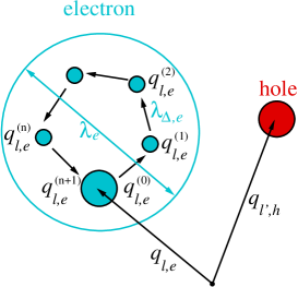
Figure 1: (Color online) Beads representation of electrons and holes. Here $\lambda_{e}^{2}=2\pi\hbar^{2}\beta/m_{e}$, $\lambda_{\Delta,e}^{2}=2\pi\hbar^{2}\Delta\beta/m_{e}$, $q^{(1)}_{l,e}=q^{(0)}_{l,e}+\lambda_{\Delta,e}\,\eta^{(1)}_{l,e}$, and $\sigma=\sigma^{\prime}$. The holes have a similar beads representation, however $\lambda_{\Delta,h}^{2}$ is $(m_{h}/m_{e})$–times smaller, so their beads distribution is not resolved in the figure.

Figure. 1 illustrates the representation of one (light) electron and one (heavy) hole. The circle around the electron beads symbolizes the region that mainly contributes to the partition function path integral. The size of this region is of the order of the thermal electron wavelength $\lambda_{e}(T)$, while typical distances between electron beads are of the order of the electron wavelength taken at an $(n+1)$–times higher temperature. The same representation is valid for each hole but it is not shown since, due to the larger hole mass, the characteristic length scales are substantially smaller. Nevertheless, in the simulations below, the holes are treated according to the full beads representation. Details, including the treatment of the spin, are given in the Appendices.

To evaluate the density matrix, accurate results for the high-temperature approximation are necessary. As we have shown earlier FiBoEbFo01 , for sufficiently high temperature, i.e. for large number $n$ of time slices) each high-temperature factor can be expressed in terms of two-particle density matrices ($p=1,\dots,N_{a},t=1,\dots,N_{b},a,b=e,h$)

$$\rho_{ab}(q_{p,a},q^{\prime}_{p,a},q_{t,b},q^{\prime}_{t,b};\beta) = \frac{(m_{a}m_{b})^{3/2}}{(2\pi\hbar\beta)^{3}}\exp\left[-\frac{m_{a}}{2\hbar^{2}\beta}(q_{p,a}-q^{\prime}_{p,a})^{2}\right]\,$$ (2)

$$\times\exp\left[-\frac{m_{b}}{2\hbar^{2}\beta}(q_{t,b}-q^{\prime}_{t,b})^{2}\right]\exp[-\beta\Phi_{ab}]$$

with the familiar Kelbg potential Ke63 ; kelbg

$$\Phi_{ab}(x_{ab};\beta)=\frac{e_{a}e_{b}}{\lambda_{ab}x_{ab}}\,\left[1-e^{-x_{ab}^{2}}+\sqrt{\pi}x_{ab}\left(1-{\rm erf}(x_{ab})\right)\right],$$ (3)

where $x_{ab}=|q_{p,a}-q_{t,b}|/\lambda_{ab}$, and the error function ${\rm erf}(x)=\frac{2}{\sqrt{\pi}}\int_{0}^{x}dte^{-t^{2}}$. The derivation of approximation (2) and discussion of its accuracy is given in App. B.

In our DPIMC scheme we use different types of steps, where either electron (hole) coordinates $q_{t,e}$ ($q_{p,h}$) or individual electronic (hole) beads are moved until convergence of the calculated values is reached. Using periodic boundary conditions (PBC) the basic MC cell (filled yellow square in Fig. 2) is periodically repeated in $x$, $y$ and $z$ directions.

As mentioned above the main contribution to the path integral representation of the partition function comes from configurations for which the typical size of the clouds of electronic (hole) beads is of the order of the thermal wavelength of electrons (holes). At the moment our computer resources allow to consider up to about one hundred electrons and holes with several tens beads in the basic MC cell. Due to this limitation on the number of particles in the MC cell there is a restriction on the size of the MC cell for a given density.

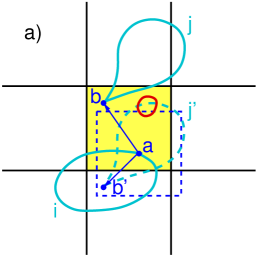
Figure 2: (Color online) Sketch of the boundary conditions used for the simulations. Electron and hole clouds of beads are denoted by solid green and red lines respectively. The dashed line shows the cell for choosing the image of particle $b$ which is closest to particle $a$. For further explanation see text.

In the case of a highly degenerate plasma the thermal wavelength and the typical size of the electronic clouds of beads may be larger than the size of the basic MC cell. So beads of electrons belonging to the basic MC cell can penetrate into neighboring images of the main cell, as well as electronic beads from a neighboring cell can extend into the basic MC cell. Due to this fact we have improved our PIMC scheme compared to previous simulations: In our new calculations we assume that an electron (hole) belongs to a certain cell if its physical coordinate $q^{0}_{t,a}(t=1,\dots,N_{a},a=e,h)$ belongs to this cell. In Fig. 2 electron and hole clouds of beads are marked by solid green and red lines. Only a few periodic images of these particles are shown by related dashed lines.

Let us consider the PBC for the calculation of pressure and energy in more detail. For distances between beads with the same number $l$ in the Kelbg potentials and its derivatives [respectively first and second line in curly brackets in Eqs. (20) and (24)] we used the standard PBC (see Fig. 2 a). Namely, in the Kelbg potential and its derivatives, instead of the distance $\overline{ab}$ between beads with the same number $l$ of electrons $i$ and $j$ we take the smallest distance $\overline{ab^{\prime}}$ to one of the electron images $j^{\prime}$. The same applies to electron-hole and hole-hole distances. Furthermore, in calculations of the scalar products and derivatives of the Kelbg potential [terms $C$ and $D$ in Eq. (20) and terms $A$ and $B$ in Eq. (24)] the situation is more complicated due to the dependence of the scalar products on the angle between vectors to beads of the particle from the basic MC cell and its periodic images. In our calculations we first of all choose, for a given particle $i$, the nearest image $j^{\prime\prime}$, according to the distance between coordinates $q^{0}_{i,e}$ and $q^{0}_{j^{\prime\prime},e}$ only, as shown in Fig. 2 b). $\overline{ab^{\prime\prime}}$ is the smallest distance for all $ab$. Then for this pair $i,j^{\prime\prime}$ we calculate all scalar product terms $A,B,C,D$ and the related derivatives of the Kelbg potential. The same is done for electron-hole and hole-hole pairs.

In our previous calculations determinants of the exchange matrices [cf. Eq. (23) of App. B] were only computed for particles belonging to the basic Monte Carlo cell. However, with increasing degeneracy $(n\lambda^{3})$ the ratio of the particle thermal wavelength to the size of the Monte Carlo cell also increases. If this ratio approaches one exchange effects between particles in the main MC cell and their images in the neighbor cells have to be included. Therefore, in the present calculations we take into account the exchange interactions of electrons and holes from neighboring Monte Carlo cells, namely first from the ($3^{3}-1$) nearest-neighbor cells, then from the $5^{3}-1$ next nearest-neighbor cells and so on. These improved calculations were tested for both an ideal plasma and a non-ideal hydrogen plasma. Excellent agreement with the known analytical results for an ideal plasma was found up to densities where the parameter $n\lambda^{3}$ reaches values of several hundreds.

In the present simulations of dense electron-hole plasmas, we varied both the particle number and the number of beads. We found that in order to obtain convergent results for the thermodynamic properties in the density-temperature range considered below it is sufficient to simulate systems with particle numbers of $N_{e}=N_{h}=50\dots 100$. Of course, the accuracy is strongly affected by the number of beads $n$. To exclude an $n$-dependence of our calculations, the density matrices in the high-temperature decomposition were always taken at temperatures above the exciton binding energy. In practice, a number of about $n=20$ beads turn out to be sufficient. In order to simplify the computations further, we included only the dominant contribution in the sums over the total electron and hole spin, which corresponds to $s=N_{e}/2$ electrons and $k=N_{h}/2$ holes having spin up and down, respectively. The contribution of the other terms is small and vanishes in the thermodynamic limit. Let us emphasize that for all results presented below the maximum statistical error is about $5\%$, which is sufficient for the present analysis. Note that this accuracy can be achieved at an acceptable cost of computer time. Of course, the error can be systematically reduced by increasing the length of the Monte Carlo run.

III Simulation results

We now apply the theoretical scheme developed in the preceding sections to a partially ionized dense electron-hole plasma. We will be interested in strong Coulomb correlation effects such as bound state (excitons, bi-excitons, clusters), their modification by the surrounding plasma and their eventual breakup at high densities due to pressure ionization (Mott effect). Beyond the Mott density, we expect the possibility of hole crystallization if the hole mass is sufficiently large Bonitz_PRL05 . To detect these effects, we have extended our first-principle DPIMC simulations to a large range of mass ratios, temperatures and densities. Below, the density of the two-component plasma is characterized by the Brueckner parameter, $r_{s}=d/a_{B}$, defined as the ratio of the mean distance between particles $d=[3/4\pi(n_{e}+n_{h})]^{1/3}$ and the exciton Bohr radius $a_{B}=\hbar^{2}\varepsilon/e^{2}m_{r}$, where $n_{e}$ and $n_{h}$ are electron and hole densities, respectively, and $\varepsilon$ is the background dielectric constant. In what follows we compute and discuss the spatial particle configurations, the pair distribution functions, static structure factors, fractions of electrons and holes in bound states, the internal energy and the equation of state.

III.1 Electron hole plasma with small/large mass ratio $M$

Let us first discuss Coulomb correlations in two-component plasmas for the limiting cases of small and very large mass ratios. In Figs. 3,4 we show data for $M=1$ (positronium, left columns in the two figures) and $M=952$ (right columns, illustrating the situation typical for hydrogen and plasmas of other chemical species). In addition, we consider the cases of small and large density, corresponding to $r_{s}=10$ (upper row) and $r_{s}=0.33$, (lower row in Figs. 3 and 4) respectively, and temperatures well below the the exciton binding energy $E_{B}=e^{2}/2\varepsilon a_{B}$. To allow for a direct comparison with the Tm[Te,Se] system below, we fix the effective electron mass to $m_{e}=2.1m_{0}$ ($m_{0}$ is the free electron mass) and the background dielectric constant to $\varepsilon=25$ which leads to a binding energy $E_{B}/k_{B}=517K$ being two orders of magnitude smaller than for positronium and hydrogen.

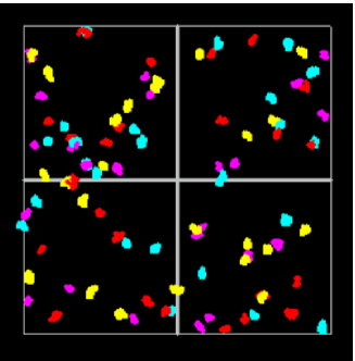
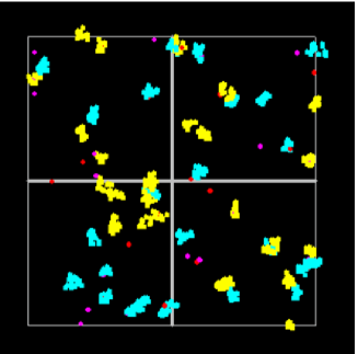
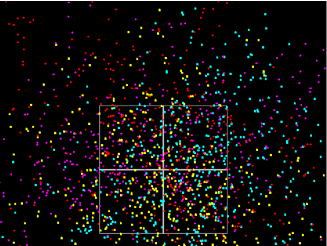
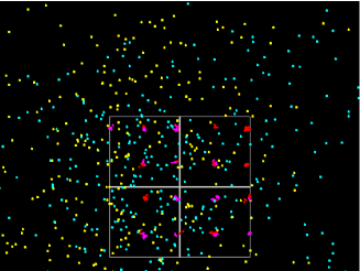
Figure 3: (Color) Snapshots of the electron-hole plasma configuration in the simulation box for two mass ratios, left (right) column: $M=1,T=100K$ ($M=952$, T=50K) and two densities corresponding to, upper (lower) row: $r_{s}=10$ ($r_{s}=0.33$). Spin up and spin down electrons (holes) are marked by yellow and blue (red and pink) clouds of dots, respectively, and the Monte Carlo cell is given by the gray grid lines (PBC were used).

In Fig. 3 we present typical spin-resolved “snapshots” of the electron-hole state in the simulation box for small and large $M$ (left and right columns, respectively). One clearly sees the influence of the hole mass on the particle probability distribution (corresponding to the DeBroglie wavelength): In the left part, electron and hole “clouds” have the same size, whereas in the right part, holes have practically shrunk to dots (negligible size compared to the interparticle distance). Let us first concentrate on the low-density limit, $r_{s}=10$, upper row in Fig. 3. At this density Coulomb correlations are strong enough to give rise to bound states - excitons. They are clearly visible in the snapshots from pairwise clustering of electrons and hole “clouds´´ for both, small and large mass ratios. Occasionally, also clusters of three or four particles are seen which correspond to trions (exciton ions) and bi-excitons, respectively.

A quantitative analysis of the behavior is obtained by computing the pair distribution functions (PDF) which are shown in the upper row of Fig. 4. They are computed in the simulations from the density operator according to

$$g_{ab}(r)=\frac{N_{e}!N_{h}!}{Z}\sum_{\sigma}\int\limits_{V}dq\,\delta(r_{1,a}-q_{1,a})\,\delta(r_{2,b}-q_{2,b})\,\rho(q,\sigma;\beta)\,.$$ (4)

For both mass ratios we observe a clear peak of $r^{2}g_{eh}$ at about $r_{eh}=1a_{B}$, corresponding to excitons. For the large mass ratio, Fig. 4b), the peak is substantially higher which is a consequence of the increase of the binding energy by a factor two compared to the case $M=1$ (the reduced mass increases from $m_{e}/2$ to $m_{e}$) which stabilizes the bound states. This trend is also seen in the snapshots (upper panel): The fraction of electron “clouds” closely attached to holes is significantly higher in the right figure. Further, the h-h PDF for the large mass ratio, Fig. 4b), show signatures of bi-exciton formation with a peak distance of about $1.4a_{B}$. Also the e-e PDF shows peaks, one at lower distances, correspponding to electrons with different spin projections located between the holes and a weaker pronounced one at larger distances. These peaks are not seen for $M=1$.

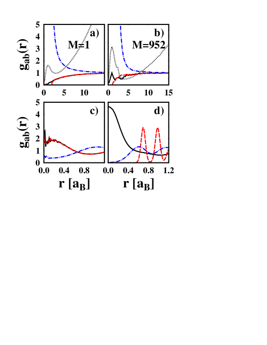
Figure 4: (Color online) Pair distribution functions (PDF) for the four combinations of mass ratio and density shown in Fig. 3, i.e., Fig. a): $M=1$, $r_{s}=10$, b): $M=952$, $r_{s}=10$, c): $M=1$, $r_{s}=0.33$, d): $M=952$, $r_{s}=0.33$. Full black lines: e-e PDF, dashed red lines: h-h PDF, dash-dotted blue lines: e-h-PDF, dotted black line: $r_{eh}^{2}g_{eh}(r_{eh})$. Distances are in units of the exciton Bohr radius $a_{B}$, note the different scales in the upper and lower row.

Let us now turn to the limit of high densities, lower row in Figs. 3 and 4. Here the influence of the mass ratio is even more dramatic, leading to a qualitative change of the plasma behavior. While the electrons are practically delocalized over the whole simulation volume for both $M$, the behavior of the holes changes from delocalized (small mass ratio; lower left part of Fig. 3) to fully localized (large mass ratio; lower right part). Obviously, in both cases no bound states exist. Instead, we observe a Fermi gas-like state of electrons and holes, at small $M$, and a hole crystal which is embedded into an electron Fermi gas, at large $M$. This interpretation is confirmed by the behavior of the PDF (lower row of Fig. 4). They are almost structureless at small $M$. In contrast, at large $M$, pronounced peaks at finite $r$ are visible in the hole-hole PDF being typical for a crystalline structure Bonitz_PRL05 .

Thus, Figs. 3 and 4 allow us to conclude that in order to observe a crystal of charged particles (hole crystal) in a two-component quantum plasma, three requirements have to be fulfilled: (i) sufficiently low temperature, (i) sufficiently high density (which causes pressure ionization of the bound states) and (iii) a large mass ratio. Below, these requirements will be studied more in detail.

The most interesting question is the role of the mass ratio. Crystals of ions (e.g. nuclei of carbon and oxygen) in the presence of a quantum electron gas are commonly accepted to exist in astrophysical objects such as White Dwarf stars segretain , where the mass ratio is of the order $M\sim 10^{4}$. But ion crystallization is expected to be possible also for much smaller mass ratios: proton crystallization ($M=1836$) in dense hydrogen has been found in our previous simulations filinov-etal.00jetpl , see also Ref. militzer06 , and we have also found crystals of alpha partilces in pure helium Bonitz_PRL05 . Figs. 3 and 4 indicate that crystallization of holes should be possible even for $M$ below 1000. Two-component plasmas with $M<1000$ exist in condensed matter systems, such as semiconductors. In most traditional semiconductors, however, typical values of $M$ are $3\ldots 20$. There have been predictions of the possibility of $M\sim 100$ in CuCl or Bi-Sb alloys under pressure, e.g. rice68 ; abrikosov78 , but without experimental evidence so far.

III.2 Thermodynamic properties of electron hole plasmas with $M=40$

The largest mass ratios in condensed matter systems were experimentally reported by Wachter and co-workers wachter for the intermediate valent $\rm Tm[Se_{x}Te_{1-x}]$ alloys under pressure. In these materials f-d-hybridization provides a narrow dispersive f-valence band and, as a consequence, a large effective hole mass of the order of 50-100 (bare) electron masses. This system is of particular interest because of the long life time of the electron-hole plasma. Moreover the mass ratio is close to the predicted critical value of $M\approx 80$ for hole crystallization Bonitz_PRL05 .

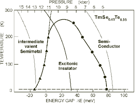
Figure 5: Excitonic phase diagram of ${\rm TmSe_{0.45}Te_{0.55}}$ taken from Ref. wachter . Measured points are designated by symbols. “Isobars” in the semi-conducting and semi-metallic phase are marked as dotted lines, whereas the “isobar” entering the excitonic phase is denoted by a full line. The lower abscissa gives the corresponding energy gap $\Delta E$ (here negative values refer to the metallic state). The left boundary (at high pressure) of the exciton-rich phase corresponds to the pressure ionization (Mott effect). For more details see Ref. wachter ; BF06 .

$\rm TmSe_{0.45}Te_{0.55}$ at ambient conditions is an indirect semiconductor with a gap of $E_{\Delta}=130$ meV. An excitonic level has been observed with $E_{B}\simeq 50-70$ meV below the bottom of the d-band. Applying pressure the gap can be tuned (and even closed), and the material is speculated to realize in the pressure region between 5 and 11 kbar an excitonic insulator, at least at very low temperatures BF06 , the search for which has been run for a long time rice68 (see the experimental phase diagram in Fig. 5). A necessary pre-condition is the existence of a large number density of (up to $10^{20}-10^{21}$ per cc) excitons of intermediate size (in order to avoid too strong overlap of the excitonic bound states) wachter . For pressures exceeding 11 kbar exciton ionization has been observed as a result of the Mott effect. This is the region in phase space where hole crystallization should occur.

In the following, we analyze this interesting system more in detail performing direct PIMC simulations within the parabolic band approximation. While this is certainly a strongly simplified model, we expect that the main trends, related to density and temperature variation, will be reproduced. The simulations were performed for an e-h plasma with $m_{e}=2.1m_{0}$ ,$m_{h}=80m_{0}$, and $\varepsilon=25$. Several characteristic temperatures within the interval of the measurements by Wachter et al. wachter ($T\lesssim 300K$) are chosen, which are well below the exciton binding energy.

III.2.1 Pressure and internal energy

We first consider the behavior of pressure $p$ and internal energy $E$ which are determined in our simulations exploiting formulas (24) and (20), derived in the App. B. Figure 6 shows $p$ and $E$ versus the Brueckner parameter (i.e. versus density to the power $-1/3$) at several fixed temperatures. At low densities and high temperature ($300$K), $p$ and $E$ reflect the classical ideal gas behavior. Reduction of density or/and temperature lead to a significant deviation from this behavior: Now $p$ and $E$ decrease due to the (overall attractive) Coulomb interaction in the plasma and, in particular, due to bound state formation of excitons and biexcitons, reaching a minimum around $r_{s}\sim 2\dots 4$. For higher densities, $p$ and $E$ start to increase again monotonically. This is triggered by quantum effects - the plasma behaves as a Fermi gas. At the same time, bound states are expected to break up as a consequence of the Mott effect. The behavior of bound states will be verified below from the snapshots and pair distribution functions. The negative values of $p$ observed at the lowest temperature point towards an instability of the homogeneous plasma state against formation of droplets or clusters. Electron-hole droplet formation in semiconductors is well established and was observed experimentally three decades ago keldysh . This effect is similar to the so-called plasma phase transition discussed by many authors for dense hydrogen and other plasmas (see norman_starostin ; Pade85 ; sbt95 ; BeEb99 ; filinov-etal.01jetpl and references therein).

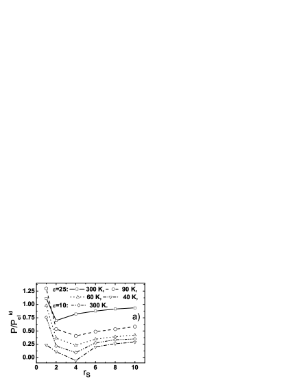
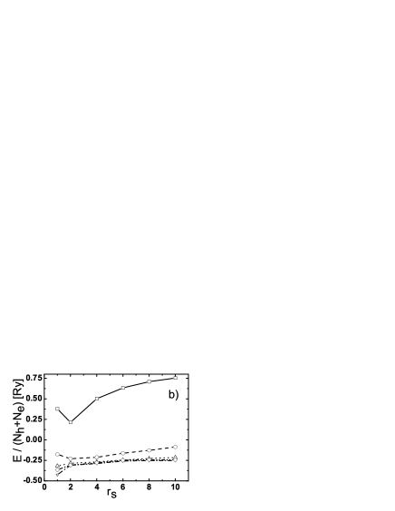
Figure 6: Isotherms of pressure and internal energy versus Brueckner parameter ($r_{s}\sim n^{-1/3}$) for an e-h-plasma with $m_{e}=2.1m_{0}$, $m_{h}=80m_{0}$ and $\varepsilon=25$. For comparison, also results for $\varepsilon=10$ at $T=300$K are shown. Pressure is in units of the classical ideal pressure, $P^{id}_{cl}=(n_{e}+n_{h})k_{B}T$.

III.2.2 Particle configurations

Figure 7 shows snapshots of the electron-hole configuration in the simulation box at different temperatures and densities. According to the temperature decomposition of the density matrix, each electron and hole is represented by several beads. We used $n=20$ beads, so for the upper panels, at $T=50$ K, the high-temperature density matrices are taken at a temperature of $1000K$, being two times larger than $E_{B}$. The spatial distribution of the beads of each quantum particle is proportional to its spatial probability distribution. Figure 7 indicates that for $M\approx 40$ the typical size of the cloud of beads for electrons is several times larger than the one for the holes. Note, that in the present strongly correlated system, the extension of electron and hole probability densities maybe quite different from the deBroglie wavelength which corresponds to the ideal case.

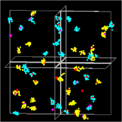
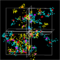
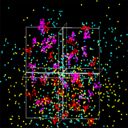
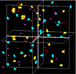
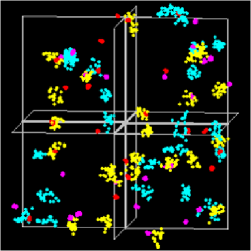
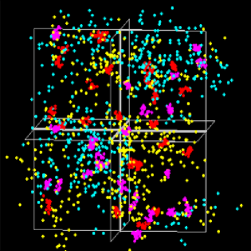
Figure 7: (Color) Snapshots of particle configurations at three particle densities corresponding to $r_{s}=10$ (left), $r_{s}=4$ (center), and $r_{s}=1$ (right). Spin up and spin down electrons (holes) are marked by yellow and blue (red and pink) clouds of dots, and the Monte Carlo cell is given by the gray grid lines (PBC were used). Upper and lower panels show results at low ($T=50K$) and high ($T=200K$) temperatures, respectively.

At low density ($r_{s}=10$, left column) and temperature $T=50K$, practically all holes are closely covered by electron beads, which means that electrons and holes form bound states, and the e-h plasma consists mainly of excitons. This interpretation will again be supported by the behavior of the pair distribution functions discussed below. Raising the temperature at fixed density leads to a (temperature-induced) ionization of the bound states. As a result we find a substantial number of free electrons and holes in the simulations (the degree of ionization will be shown in Fig. 11 below).

For intermediate densities ($r_{s}=4$, middle column) we observe the formation of bi-excitons and many-particle clusters at low temperatures ($T=50K$). Now the electron-hole system is strongly inhomogeneous. In this case the mean distance between particles $d$ is of the order of the electron wavelength. At $T=200K$ bi-excitons and many-particle clusters are absent due to thermal break up of exciton-exciton bound states.

At high density ($r_{s}=1$) the electron wavelength exceeds the mean inter-particle distance $d$ and even the size of the Monte Carlo cell used in the simulations, which is seen by the large extension of the electron beads clouds. At the same time excitons become unstable because two electrons bound to neighboring holes start to overlap allowing for electron tunneling from one exciton to another (pressure ionization, Mott effect), and the system transforms into a plasma of electrons and holes. Since the hole wavelength is significantly smaller than the electron wavelength (and may still be smaller than $d$), in a certain region of $r_{s}$-values the structure of the hole beads resembles a liquid state (lower right panel).

III.2.3 Pair distribution functions and structure factors

Now let us discuss the behavior of the spin-averaged electron-electron-, hole-hole- and electron-hole PDFs defined in Eq. (4). Figure 8 shows the three functions $g_{ab}(r)$ versus the inter-particle distance $r=r_{1,a}-r_{2,b}$ for the same densities and temperatures as in Fig. 7. Here no smoothening has been carried out, i.e. the fluctuations of $g_{ee},$ $g_{hh}$ and $g_{eh}$ at small $r$ reflect the magnitude of the statistical errors of our simulation.

     

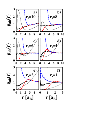
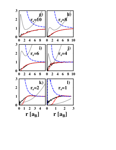
Figure 8: (Color online) Pair distribution functions $g_{ee}$ (black solid line), $g_{hh}$ (red dashed line), and $g_{eh}$ (blue dot-dashed line) at $T=50K$ (left two columns) and $T=200K$ (right two columns). The dotted lines show $r^{2}g_{eh}$ where, for better visibility of the exciton peak, the data are divided by a factor $120$ in panels a and b, by a factor of $30$ in figures c, d, g, and h, and by a factor of $10$ in panels e, f, and i-l.

As an effect of the Coulomb and Fermi (statistics) repulsions, $g_{ee}$ and $g_{hh}$ are suppressed at small distances. Due to the large mass difference the decay of the e-e correlations, however, is essentially different from that of the h-h correlations. The asymptotic of $g_{ee}$ at small distances is determined mainly by electrons with opposite spin projections (since the strong Fermi repulsion is absent). For these electron pairs the main contribution to the repulsion comes from the effective quantum Kelbg potential (recall that it is finite at zero distance), allowing for tunneling of electrons up to zero separation. This is supported by the behavior of the spin dependent pair distribution shown in Fig. 10. Of course, the tunnelling effect are much more pronounced for the lighter electrons.

The strong peak of $g_{eh}$ at low densities ($r_{s}=10\dots 8$) is caused by excitons. This is confirmed by considering the function $r^{2}g_{eh}(r)$ which exhibits a pronounced maximum at about $1a_{B}$, i.e. at the exciton Bohr radius. At these densities, the functions $g_{ee}$ and $g_{hh}$ exhibit no peak structure, i.e. there is no indication of formation of bound exciton-exciton complexes (such as bi-excitons or electron-hole droplets). With increasing temperature more and more excitons dissociate, and the maximum of $r^{2}g_{eh}$ is reduced.

Varying, at low temperatures, the density over three orders of magnitude, the maximum of $r^{2}g_{eh}$ is suppressed and finally vanishes. At about $r_{s}=6$, there is evidence that recombination into bi-excitons takes place. At the same time, the position of the maximum in $r^{2}g_{eh}$ shifts from 1 $a_{B}$ to 2-3 $a_{B}$ approximately, indicating the increasing radii of the bound states. This scenario is confirmed by the behavior of $g_{ee}$ and $g_{hh}$: For intermediate densities ($2<r_{s}<6$), they exhibit distinct peaks at larger $r$, pointing towards the formation of bi-excitons and many-particle clusters. For $r_{s}\lesssim 1$, the fraction of excitons is further reduced due to many-body effects (pressure ionization), and bi-excitons and many-particle clusters vanish.

Finally let us relate the width of the peak of $g_{eh}$ to the extension of the ground state wavefunction ($\sim 1a_{B}$). At low densities ($r_{s}>6$) the peak of $g_{eh}$ is rather broad, indicating the population of excited states, while at high densities ($r_{s}\sim 1$) the width of the lowest peak in $g_{eh}$ becomes significantly smaller than the corresponding width of the ground-state peak. At the same time the hole-hole pair distribution function reveals an ordering of the holes into a fluid-like state.

Figure 9 shows the variation of the static charge structure factor, defined in reciprocal $k$-space as

$$S_{ab}(k) = \frac{\int_{0}^{\infty}drr^{2}(g_{ab}(r)-1)\sin(kr)/(kr)}{|\int_{0}^{\infty}drr^{2}(g_{ab}(r)-1)|}\,.$$ (5)

According to Eq. (5) positive (negative) values of $S_{ab}(k)$ indicate attraction (repulsion) in momentum space, see also Ref. fehske-ktnp05 .

     

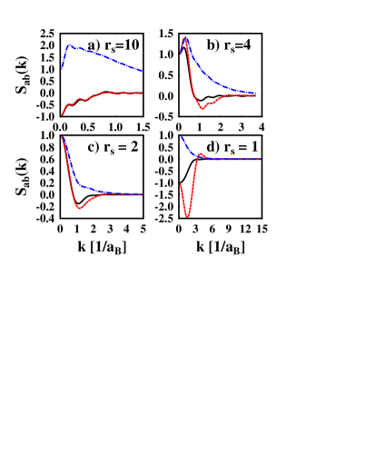
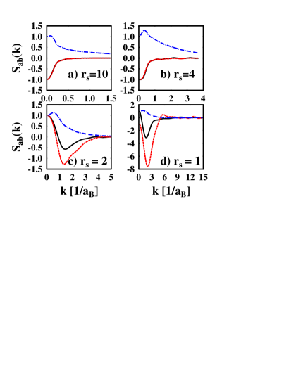
Figure 9: (Color online) Static structure factor $S_{ee}$ (black solid line), $S_{hh}$ (red dashed line), and $S_{eh}$ (blue dot-dashed line) at $T=50K$ (left columns) and $T=200K$ (right columns).

Starting at low densities ($r_{s}=10$), the negative values of the e-e and h-h structure factors at small momenta (large distances) originate from the strong Coulomb repulsion of quasi-free equally charged particles. The maximum of $S_{eh}$, as well as the modulations of $S_{ee}$ and $S_{hh}$ at finite $k$, are indicative of exciton formation. Excitons set a new length scale in the structure factor at about 0.2 [$1/2a_{B}$]. As expected, these signatures are washed out at higher temperatures, where excitons break up. At high density ($r_{s}=1$) the large mass ratio between electrons and holes is responsible for the different behavior of $g_{ee}$ and $g_{hh}$. This is especially true for low temperatures when the electrons are perfectly delocalized but the holes still have fluid-like short-range correlations as noted above. The value of the normalization constant (denominator) in Eq. (5) is responsible for the different magnitude of the $S_{hh}$ at $T=50K$ and $T=200K$.

The e-e- and h-h PDF and structure factors presented in Figs. 8 and 9 were averaged over the spin degree of freedom of the particles. Our DPIMC simulations, however, allow direct inspection of the spin effects as well. Especially for the case of large degeneracy ($n\lambda^{3}\gg 1$) we expect qualitatively different behavior of $g^{\uparrow\uparrow}_{aa}$ and $g^{\uparrow\downarrow}_{aa}$ at small distances, due to the influence of the Fermi statistics ($a=e,h$). This is confirmed by Fig. 10. In other words, we clearly see the exchange-hole known from the ideal Fermi gas, but here it appears in a strongly interacting e-h plasma. In contrast, for the much heavier holes the quantum statistical repulsion is much less pronounced, and the decay of $g_{hh}$ for $r\to 0$ is mainly triggered by the (spin-independent) Coulomb interaction.

     

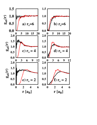
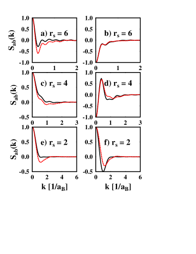
Figure 10: (Color online) Spin resolved pair distribution functions $g_{ab}(r)$ and structure factor $S_{ab}(k)$ for electrons (solid black lines) and holes (dashed red lines) at $T=50$ K. Left (right) columns correspond to antiparallel (parallel) spin projections of the particle pair.

The snapshots depicted in Fig. 7 have shown that in the density regime $2\leq r_{s}\leq 6$ the plasma contains a large fraction of bi-excitons. Now, Fig. 10 confirms this conclusion (consider, e.g., the case $r_{s}=4$): There is not much difference in $g^{\uparrow\uparrow}_{hh}$ and $g^{\uparrow\downarrow}_{hh}$ - both functions exhibit a similar peak at a hole-hole distance of about $3a_{B}$. In contrast, the electron behavior is strongly spin dependent: There is a high probability to encounter two electrons with different spin projections between two holes (at a distance $1a_{B}\dots 2a_{B}$) – which is the expected behavior known from bi-excitons (or the hydrogen molecule).

The corresponding charge structure factors clearly show that the difference between electrons and holes with respect to the spin correlations are most pronounced in the regime where bound states are formed but, of course, the differences are less important at very small and large $k$ (corresponding to large and small distances, respectively). We found attraction (repulsion) for opposite (equal) spin projections for both particles as $k\to 0$, except for the case of high densities, where the hole fluid forms. Here, in the vicinity of the Mott transition, the difference between the structure factor for electrons and holes with same and opposite spin projections is notably smaller; they are close to their spin-averaged values given in Fig. 9 for $T=50$ K and $r_{s}=2$.

III.2.4 Degree of ionization. Mott density

The above analysis of the snapshots and PDFs has indicated that, in a broad range of densities, the e-h-plasma is partially ionized containing a varying fraction of free and bound electrons and holes. The value of the critical Mott density (corresponding to the Brueckner parameter $r_{s}^{\rm Mott}$) where excitons vanish due to pressure ionization is essential for the occurrence of hole crystallization. In particular, the critical mass ratio was found to directly depend on $r_{s}^{\rm Mott}$ as $M^{cr}+1=r_{s}^{cr}/r_{se}^{\rm Mott}$, where $r_{se}\equiv 2^{1/3}r_{s}$ and $r_{s}^{cr}\approx 100$ is the critical value for Coulomb crystallization in a one-component plasma rsc_ocp . The value of $r_{s}^{\rm Mott}$ depends in a complicated way on the structure of the excitons (which may be quite different for different materials) and on many-body effects such as screening and bound-state renormalization. This is a very complex problem which has been discussed in a variety of approximations the accuracy of which, however, is difficult to assess (see e.g. Ref. green-book for an overview). Based on our DPIMC simulations avoiding any simplifying assumptions, we have the possibility to obtain a consistent many-body result for $r_{s}^{\rm Mott}$. To this end, we first need to find a definition for the degree of ionization which is applicable to our simulations.

The main problem of PIMC simulations in configuration space is that there is, in principle, no clear subdivision into bound and free “components” possible. Electron-hole correlations arising from bound and scattering states contribute to the same quantities, such as energy, equation of state or PDF. Note that the usual subdivision in energy space into bound and scattering states according to negative and positive relative pair energies $E_{\alpha}$ also breaks down in the case of strong correlations: Eigenvalues $E_{\alpha}$ and wavefunctions $\Psi_{\alpha}(r)$ are being renormalized, $\Psi_{\alpha}\rightarrow{\tilde{\Psi}}_{\alpha};E_{\alpha}\rightarrow{\tilde{E}}_{\alpha}$. In the vicinity of the Mott point, the distinction between bound and scattering states becomes meaningless, bound state levels merge into the scattering continuum green-book .

Nevertheless, a rough estimation of the fraction $1-\alpha^{ion}$ of e-h bound states ($\alpha^{ion}$ denotes the degree of ionization) can be obtained by analyzing the PDF $g_{eh}$. In particular, at low temperatures $k_{B}T\ll E_{B}$ and far below the Mott density, the plasma will consist of excitons in the ground state $E_{1}$, i.e. $g_{eh}(r)\sim|\Psi_{1}(r)|^{2}$ (see filinov-etal.00pla ). In the general case, the PDF will contain a superposition (mixed state) of all renormalized eigenfunctions, weighted with the Boltzmann factor,

$$g_{eh}(r)\sim\sum_{\alpha}|{\tilde{\Psi}}_{\alpha}(r)|^{2}\exp(-\beta{\tilde{E}}_{\alpha}).$$ (6)

While the scattering states are delocalized, the bound state wavefunctions are localized in space leading to an increase of $g_{eh}$ beyond the result for an ideal plasma $g^{id}_{eh}\equiv 1$. Due to the normalization of $g_{eh}$ values of $g_{eh}>1$ at small e-h distances must be compensated by a depletion, $g_{eh}<1$, at larger distances. Now, recall that $g_{eh}$ is related to the probability density by $P_{eh}(r)\sim r^{2}g_{eh}(r)$ which, in the case of excitons, is strongly enhanced around $r_{eh}=1a_{B}$, cf. Fig. 8. Hence we can use as a “pragmatic” definition of the fraction of bound states (this idea is due to N. Bjerrum who used it very successfully in the theory of electrolytes bjerrum ) the probability of e-h-pairs being at small distances (where $g_{eh}>1$):

$$\frac{N_{eh}^{b}}{N_{eh}^{b}+N_{eh}^{c}}\equiv 1-\alpha^{ion}\approx\frac{\int_{0}^{r^{b}}r^{2}\,[g_{eh}(r)-1]\,dr}{\int_{0}^{r^{b}}r^{2}\,g_{eh}(r)\,dr}\,.$$ (7)

Here $r_{b}$ is the second zero of $r^{2}(g_{eh}-1)$ which is located to the right of the exciton peak. By subtracting $\int_{0}^{r^{b}}r^{2}\,dr$ in the nominator, the uncorrelated contributions are eliminated from the full probability density. The denominator accounts for the normalization (giving the full probability of particles being in bound or scattering states). Of course, this definition is only qualitative since it does not exclude attractive scattering states and thus may slightly overestimate the “true” bound state fraction.

An analogous ratio can be defined for the hole-hole bound-state (bi-exciton) fraction

$$\frac{N_{hh}^{b}}{N_{hh}^{b}+N_{hh}^{c}}=\frac{\int_{r^{b^{\prime}}}^{r^{b}}r^{2}\,[g_{hh}(r)-1]\,dr}{\int_{r^{b^{\prime}}}^{r_{b}}r^{2}\,g_{hh}(r)\,dr},$$ (8)

with $[r^{b^{\prime}},r_{b}]$ being the interval where $r^{2}\,(g_{hh}(r)-1)$ is positive.

We expect that the definition (7) is well suited for a numerical determination of the Mott density as the density, where the plasma becomes dominated by free particle behavior. We will identify $r_{s}^{\rm Mott}$ as the density where the bound state fraction falls below $5\dots 10\%$, i.e. $\alpha^{ion}=90\dots 95\%$.

Figure 11 presents our DPIMC results for the e-h bound state fraction according to Eqs. (7), (8). At low densities ($r_{s}>6$) and low temperatures ($T<100$ K) practically all electrons and holes are bound in excitons, i.e. bi-excitons and many-particle clusters are absent. Increase of temperature, $T\geq 100K$, leads to a strong ionization of excitons, i.e. free particles dominate. In the intermediate density regime ($2<r_{s}<6$) and for low temperatures ($T<100$ K), the largest fraction (up to about $20\%$) of h-h bound states (bi-excitons and many-particle clusters) is observed. It is interesting to note that at higher temperatures ($T\sim 100$K$\dots 300$ K) the exciton fraction increases a bit for higher density.

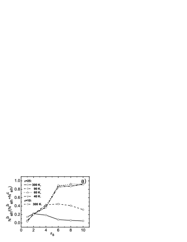
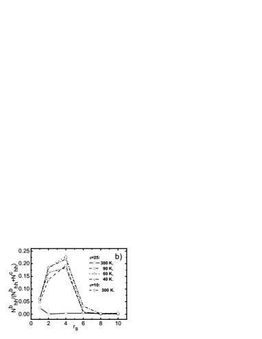
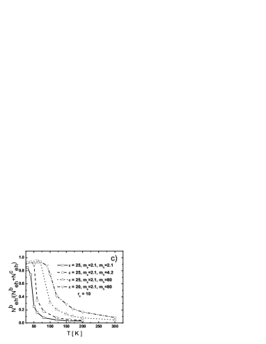
Figure 11: Fraction of the electron-hole (top left, a)) and hole-hole bound states (top right, b)) versus Brueckner parameter $r_{s}$ for different temperatures and dielectric constants. Bottom Fig. (c) illustrates the temperature induced break up of excitons for different mass ratios and dielectric constants.

A decrease of the bound state fraction below $5\%$ is observed for $r_{s}\approx 1$ which we, therefore, identify with the Mott density, $r_{s}^{\rm Mott}\approx 1$ with an error of about $30\%$ (which corresponds to $r_{se}\approx 1.2$ which was used in Ref. Bonitz_PRL05 ). From this result, we confirm the value of the critical mass ratio (see above) $M^{cr}\approx 83$ which is in the range of previous predictions, e.g. mcr_data . Since also the value for $r_{s}^{cr}$ is expected to have an error of about $20\%$, a total uncertainty of about $50\%$ has to be expected. This means that hole crystallization might occur already below $M\approx 80$ which underlines again the interest in the ${\rm Tm[Se_{x}Te_{1-x}]}$ system.

Let us, therefore, come back to the experimental phase diagram, Fig. 5. There the excitonic-rich phase should exist up to a temperature of about $250$K. Then it is of course interesting to calculate the temperature dependence of the e-h bound state fraction in this regime (cf. the results for $r_{s}=10$, bottom part Fig. 11). Although our simulations do not exhibit a sharp transition from an excitonic to an ionized “phase”, we can again formally use a bound state fraction of 10 % as the boundary of the exciton dominated phase. Then, at low density, e.g. for $r_{s}=10$, these bound states will be stable up to $T=150\dots 250$ K. Note that these values are quite sensitive to $\varepsilon$ which is not precisely known. We therefore have performed simulations for two slightly different values. Increase of $\varepsilon$ leads to a more weakly bound excitons and consequently reduces the ionization temperature. The same tendency is observed if the mass ratio $M$ is lowered. Fig. 11 shows that the ratio of temperatures corresponding to $\alpha^{ion}=50~{}\%$ is the same as the corresponding ratio of the reduced masses $m_{r}=m_{e}m_{h}/(m_{e}+m_{h})$ (keeping $\varepsilon$ fixed). For example, a ratio of about 2 is observed for the data belonging to $m_{h}=80$ and $m_{h}=2.1$, and 1.5 for those belonging to $m_{h}=80$ and $m_{h}=4.2$. Clearly, as expected for an isolated exciton, the binding energy is proportional to $m_{r}$. Note however that in the present case the excitons are embedded into an e-h plasma which influences the bound state spectrum, so the recovery of the single exciton behavior is not a trivial result.

We can also give a rough estimate of the critical electron density where the transition from an insulator (built up of e-h bound states) to a (semi-) metal takes place, again using a value of $\alpha^{ion}=90\%$ as a criterion. The critical value of $r_{s}\sim 1$ corresponds to a particle density of the order of $10^{21}$ cm^-3 which is in reasonable agreement with the estimates from the experiments.

III.3 Increased hole localization with increasing mass ratio

After we have confirmed the pressure induced break up of excitons and determined the Mott parameter $r_{s}^{\rm Mott}$ in ${\rm Tm[Se_{x}Te_{1-x}]}$ with a mass ratio of $M\approx 40$, we can now return to the question of strong h-h correlations at high density and the possibility of hole crystallization. To this end we have performed DPIMC simulations at low temperatures and high densities, well above the Mott point, and varied the mass ratio over two orders of magnitude.

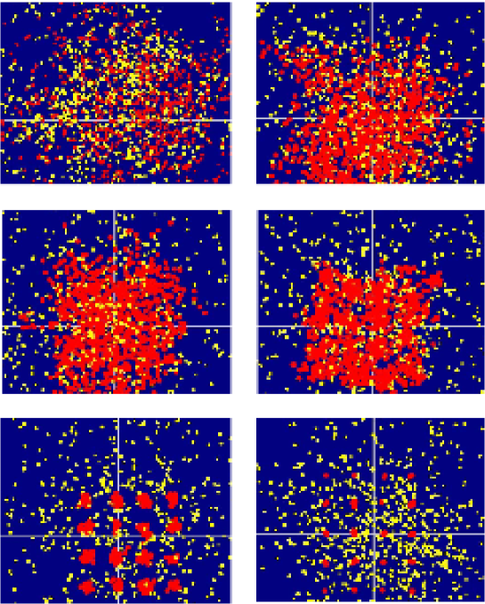
Figure 12: (Color) Snapshots of the electron-hole plasma at high density ($r_{s}=0.5$) and $T/E_{B}=0.064$. The pictures show the spin-averaged electron (yellow) and hole (red) beads configuration for different values of the mass ratio $M$ (from top left to bottom right): 5, 12, 25, 50, 100, 400.

Fig. 12 shows the results for $r_{s}=0.5$ and $k_{B}T/E_{B}=0.064$ with $M$ ranging from $5$ to $400$. To simplify the analysis we do not mark electrons and holes having different spin projections with different colors (we found that, for hole crystallization, spin effects are of minor importance). Since the density is an order of magnitude higher than the Mott density, electrons and holes are in the plasma state. For all values of $M$ the electrons are completely delocalized, forming a Fermi gas which is very weakly correlated. At the same time, the nature of the hole state changes drastically increasing of $M$. Initially ($M=5$), the holes are also in a Fermi gas-like state where individual holes penetrate each other. An increase of $M$ up to $50$ leads to continuous growing hole localization. At $M=50$ individual holes can be distinguished: Their DeBroglie wavelength $\lambda_{h}$ becomes smaller than the average distance between two holes $d_{h}$. A further increase of $M$ to 100 leads to an additional reduction of $\lambda_{h}$ by a factor $\sqrt{2}$ (with $d_{h}$ unchanged) and, consequently, to hole localization. The holes form a regular lattice - a Coulomb crystal (bottom left Fig.). Increasing the mass ratio further, the lattice becomes more rigid (bottom right Fig.), until the holes become practically point-like (cf. Fig. 4). Based on these simulation results we can conclude that, at these values of density and temperature, hole crystallization occurs between $M=50$ and $M=100$, which is in surprisingly good agreement with the analytical estimate for $M^{cr}$ based on the Mott density obtained above for the same parameters.

Obviously, the snapshots allow for a very rough determination of the critical mass ratio only. A more accurate estimate can be obtained by analyzing the relative distance fluctuation of the holes in dependence on $M$. These results, reported in Ref. bonitz-etal.06jpa , confirm the above result for $M^{cr}$. We also have studied the thermal properties of the hole crystal which arise to a temperature dependence of $r_{s}^{\rm Mott}$. As seen from Fig. 11 (left part) the bound state fraction isotherms has reached saturation at about $60$K (corresponding to slightly more than $0.1E_{B}$). Thus our result for $M^{cr}$ will not change significantly at lower temperatures, thus reflecting the ground state behavior. The full phase diagram of the hole crystal was published in Ref. Bonitz_PRL05 .

IV Discussion

In this paper we have presented a numerical (computer simulation) analysis of strong Coulomb correlations in dense three-dimensional two-component plasmas at rather low temperatures. We were in particular interested in systems with a mass ratio $M\sim 40$ which is intermediate between “usual” semiconductors ($M\sim 2\dots 10$) and “conventional” plasmas (such as hydrogen with $M\geq 1836$). Two-component Coulomb systems with this mass ratio behave in many aspects like plasmas, with the main difference that quantum and spin properties of the heavy particles (holes) cannot be neglected. Such systems might be realized in intermediate valence semiconductors under pressure.

From a plasma physics standpoint these are very interesting materials because they allow to investigate nontrivial high density phenomena of current interest, such as pressure ionization (Mott effect), plasma phase transition and metal-insulator transition. These effects exist in “conventional” plasmas only above a density of the order of $1$g cm^-3 which, meanwhile, can be achieved in laser or ion beam compression experiments, however, only for short periods of time which makes precision measurements of the plasma properties very difficult. The same physical effects can be observed in the above mentioned semiconductor materials under stationary (equilibrium) conditions at densities and temperatures which are easily accessible in experiments. In fact, the (qualitative) phase diagrams of dense plasmas and electron-hole plasmas are readily translated from one to another by rescaling the binding energy and the Bohr radius bonitz_pj02 ; bonitz-etal.03jpa . For this reason, the phase diagram of Tm[Se,Te], shown in Fig. 5, is of interest also for the physics of dense partially ionized plasmas.

In this paper, we concentrated on the central part of this phase diagram, where a large fraction of bound states exists, on the Mott transition and on the high density effects (hole crystallization). A theoretical treatment of these effects is very difficult, because many-body effects such as bound state formation, screening and quantum effects have to be taken into account self-consistently. While for such complex systems analytical methods fail, our first principle path integral Monte Carlo approach is well suited. In order to avoid additional approximations which are particularly questionable in the region of the Mott point, we have used direct fermionic simulations. With an improved treatment of the spin statistics we were able to present reliable simulations. Restricting the simulations to temperatures above $6\%$ of the exciton binding energy and densities to values not significantly higher than the Mott density allowed us to avoid serious difficulties arising from the fermion sign problem.

Most notably, we have shown that, above the Mott point, two-component plasmas with large mass anisotropy show interesting Coulomb correlation phenomena: with increasing density holes can undergo a phase transition to a Coulomb liquid and to a Wigner crystal which are embedded into a degenerate electron Fermi gas. Such crystals are expected to exist in White Dwarf stars where the mass ratio exceeds $10^{4}$. However, crystal formation in a two-component plasma should be possible also for the light elements, such as hydrogen filinov-etal.00jetpl ; militzer06 and helium and, more generally, for plasmas with mass ratios as low as 80 (cf. Bonitz_PRL05 ). This should be possible to achieve in the semiconductor materials announced in this paper. More subtle questions, such as the symmetry of the crystal and its energy cannot yet been answered conclusively, mainly because of the yet too small size of the simulations (50 electrons and 50 holes are presently feasible). Therefore, in order to obtain more accurate data, e.g. for the internal energy of a macroscopic two-component plasma at very high density, a significant increase of the simulation size would be highly desirable.

Appendix A Path integral representation of thermodynamic quantities

Let us consider a neutral two-component plasma consisting of $N_{e}=N_{h}=N$ electrons and holes in equilibrium with the hamiltonian, ${\hat{H}}={\hat{K}}+{\hat{U}}^{c}$, containing kinetic energy ${\hat{K}}$ and Coulomb interaction energy ${\hat{U}}^{c}={\hat{U}}_{hh}^{c}+{\hat{U}}^{c}_{ee}+{\hat{U}}^{c}_{eh}$ contributions. The thermodynamic properties in the canonical ensemble with given temperature $T$ and fixed volume $V$ are fully described by the density operator ${\hat{\rho}}=e^{-\beta{\hat{H}}}/Z$ with the partition function (1).

Pressure and internal energy follow from

$$\beta p = \frac{\partial{\rm ln}Z}{\partial V}=\left[\frac{\alpha}{3V}\frac{\partial{\rm ln}Z}{\partial\alpha}\right]_{\alpha=1},$$ (9)

$$\beta E = -\beta\frac{\partial{\rm ln}Z}{\partial\beta},$$ (10)

where $\alpha=L/L_{0}$ is a length scaling parameter.

The density matrix of interacting quantum systems is can be constructed using a path integral approach feynman-hibbs based on the operator identity $e^{-\beta{\hat{H}}}=e^{-\Delta\beta{\hat{H}}}\cdot e^{-\Delta\beta{\hat{H}}}\dots e^{-\Delta\beta{\hat{H}}}$, where $\Delta\beta=\beta/(n+1)$, which allows us to rewrite the integral in Eq. (1)

$$\sum_{\sigma}\int\limits dq^{(0)}\,\rho(q^{(0)},\sigma;\beta)=\int\limits dq^{(0)}\dots dq^{(n)}\,\rho^{(1)}\cdot\rho^{(2)}\,\dots\rho^{(n)}\times$$

$$\qquad\sum_{\sigma}\sum_{P_{e}}\sum_{P_{h}}(\pm 1)^{\kappa_{P_{e}}+\kappa_{P_{h}}}{\cal S}(\sigma,{\hat{P}_{e}}{\hat{P}_{h}}\sigma_{a}^{\prime}){\hat{P}_{e}}{\hat{P}_{h}}\rho^{(n+1)}\big{|}_{q^{(n+1)}=q^{(0)},\sigma^{\prime}=\sigma}\,.$$ (11)

The spin gives rise to the spin part of the density matrix (${\cal S}$) with exchange effects accounted for by the permutation operators $\hat{P}_{e}$ and $\hat{P}_{h}$ acting on the electron and hole coordinates $q^{(n+1)}$ and spin projections $\sigma^{\prime}$. The sum is over all permutations with parity $\kappa_{P_{e}}$ and $\kappa_{P_{h}}$. In Eq. (11) the index $k=1\dots n+1$ labels the off-diagonal high-temperature density matrices $\rho^{(k)}\equiv\rho\left(q^{(k-1)},q^{(k)};\Delta\beta\right)=\langle q^{(k-1)}|e^{-\Delta\beta{\hat{H}}}|q^{(k)}\rangle$. Accordingly each particle is represented by a set of $n+1$ coordinates (“beads”), i.e. the whole configuration of the particles is represented by a $3(N_{e}+N_{h})(n+1)$-dimensional vector $\tilde{q}\equiv\{q_{1,e}^{(0)},\dots q_{1,e}^{(n+1)},q_{2,e}^{(0)}\ldots q_{2,e}^{(n+1)},\ldots q_{N_{e},e}^{(n+1)};q_{1,h}^{(0)}\ldots q_{N_{h},h}^{(n+1)}\}$ (see Fig. 1).

To determine the energy in the path integral representation (11) each high-temperature density matrix has to be differentiated in turn (here we extend our earlier hydrogen results of Refs. FiBoEbFo01 ; zamalin ):

$$\beta E = -\frac{1}{Z}\int\limits dq^{(0)}\dots dq^{(n)}\,\sum_{\sigma}\sum_{P_{e}}\sum_{P_{h}}(\pm 1)^{\kappa_{P_{e}}+\kappa_{P_{h}}}\,{\cal S}(\sigma,{\hat{P}_{e}}{\hat{P}_{h}}\sigma^{\prime})\,$$ (12)

$$\;\times\sum_{k=1}^{n+1}\rho^{(1)}\dots\rho^{(k-1)}\left[\beta\frac{\partial\rho^{(k)}}{\partial\beta}\right]\rho^{(k+1)}\,\dots\,\rho^{(n)}{\hat{P}_{e}}{\hat{P}_{h}}\rho^{(n+1)}\bigg{|}_{q^{(n+1)}=q^{(0)},\,\sigma^{\prime}=\sigma}\,.$$

One can show that the matrix elements $\rho^{(k)}$ can be rewritten as

$$\rho^{(k)} \equiv \langle q^{(k-1)}|e^{-\Delta\beta{\hat{H}}}|q^{(k)}\rangle=\int d{\tilde{p}}^{(k)}d{\bar{p}}^{(k)}\,\langle q^{(k-1)}|e^{-\Delta\beta{\hat{U}}^{c}}|{\tilde{p}}^{(k)}\rangle\langle{\tilde{p}}^{(k)}|e^{-\Delta\beta{\hat{K}}}|{\bar{p}}^{(k)}\rangle\,$$ (13)

$$\hskip 170.71652pt\times\langle{\bar{p}}^{(k)}|\,e^{-\frac{\Delta\beta^{2}}{2}[{\hat{K}},{\hat{U}}^{c}]}\,\dots|q^{(k)}\rangle\,,$$

where ${\tilde{p}}^{(k)}({\bar{p}}^{(k)})$ are conjugate variables to $q^{(k-1)}(q^{(k)})$. Evaluating the derivatives in Eq. (12) further, it is convenient to introduce dimensionless integration variables $\eta^{(k)}=(\eta_{h}^{(k)},\eta_{e}^{(k)})$, where $\eta_{a}^{(k)}=\kappa_{a}(q^{(k)}_{a}-q^{(k-1)}_{a})$ for $k=1,\dots,n$, and $\kappa_{a}^{2}\equiv m_{a}/(2\pi\hbar^{2}\Delta\beta)=1/\lambda_{\Delta,a}^{2}$. The main advantage is that differentiation of the density matrix now affects only the interaction terms

$$\beta\frac{\partial\rho^{(k)}}{\partial\beta} = -\beta\frac{\partial[\Delta\beta\cdot U^{c}(X^{(k-1)})]}{\partial\beta}\rho^{(k)}+\beta{\tilde{\rho}}_{\beta}^{(k)},$$ (14)

where

$${\tilde{\rho}}_{\beta}^{(k)}=\int d{p}^{(k)}\,\langle X^{(k-1)}|e^{-\Delta\beta{\hat{U}}^{c}}|{p}^{(k)}\rangle e^{-\frac{\langle{p}^{(k)}|{p}^{(k)}\rangle}{4\pi(n+1)}}\,\langle{p}^{(k)}|\frac{\partial}{\partial\beta}\,e^{-\frac{(\Delta\beta)^{2}}{2}[{\hat{K}},{\hat{U}}^{c}]}\,\dots|X^{(k)}\rangle$$ (15)

with $p_{a}^{(k)}={\tilde{p}}_{a}^{(k)}/(\kappa_{a}\hbar)$, $p{(k)}\equiv(p_{h}^{(k)},p_{e}^{(k)})$, and use has been made of Eq. (13). Furthermore $X^{(0)}\equiv(\kappa_{h}q_{h}^{(0)},\kappa_{e}q_{e}^{(0)})$, $X^{(k)}\equiv(X_{h}^{(k)},X_{e}^{(k)})$ with $X_{a}^{(k)}=\kappa_{a}q_{a}^{(0)}+\sum_{l=1}^{k}\eta^{(l)}_{a}$ ($k$ runs from $1$ to $n$), and $X^{(n+1)}\equiv(\kappa_{h}q_{h}^{(n+1)},\kappa_{e}q_{e}^{(n+1)})=X^{(0)}$.

For $k=n+1$, we have

$$\beta\frac{\partial}{\partial\beta}\,{\hat{P}_{e}}{\hat{P}_{h}}\rho^{(n+1)}=-\beta\frac{\partial\Delta\beta\cdot U^{c}(X^{(n)})}{\partial\beta}{\hat{P}_{e}}{\hat{P}_{h}}\rho^{(n+1)}+\beta{\hat{P}_{e}}{\hat{P}_{h}}{\tilde{\rho}}_{\beta}^{(n+1)}\,.$$ (16)

Then, together with Eq. (12), we obtain for the energy

$$\beta E = \frac{3}{2}(N_{e}+N_{h})-\frac{1}{Z}\frac{1}{\,\lambda_{h}^{3N_{h}}\lambda_{e}^{3N_{e}}}\int\limits_{V}dq^{(0)}d\eta^{(1)}\dots d\eta^{(n)}\,$$ (17)

$$\times \sum_{\sigma}\sum_{P_{e}}\sum_{P_{h}}(\pm 1)^{\kappa_{P_{e}}+\kappa_{P_{h}}}\,{\cal S}(\sigma,{\hat{P}_{e}}{\hat{P}_{h}}\sigma^{\prime})$$

$$\times \Bigg{\{}\sum_{k=1}^{n+1}\rho^{(1)}\dots\rho^{(k-1)}\left[\beta{\tilde{\rho}}_{\beta}^{(k)}-\beta\frac{\partial\Delta\beta\cdot U^{c}(X^{(k-1)})}{\partial\beta}\rho^{(k)}\right]$$

$$\times \rho^{(k+1)}\,\dots\,\rho^{(n)}{\hat{P}_{e}}{\hat{P}_{h}}\rho^{(n+1)}\Bigg{\}}\bigg{|}_{X^{(n+1)}=X^{(0)},\,\sigma^{\prime}=\sigma}.$$

This way the derivatives of the density matrix have been calculated and we turn to the next point: Finding approximations for the high-temperature density matrices $\rho^{(k)}$.

Appendix B High-temperature asymptotics for the density matrix. Kelbg potential

In this section we discuss approximations for the high-temperature density matrix that can be used for efficient DPIMC simulations. This involves effective quantum pair potentials $\Phi_{ab}$, which are approximated by the Kelbg potential (see also previous work FiBoEbFo01 ).

B.1 Pair approximation and Kelbg potential

The N-particle high-temperature density matrix is expressed in terms of two-particle density matrices (higher order terms become negligible at sufficiently high temperature, i.e. for large number $n$ of time slices) given by (2). This results from factorization into kinetic and interaction parts, $\rho_{ab}\approx\rho_{0}^{K}\rho^{U^{c}}_{ab}$, which is exact in the classical case, i.e. at sufficiently high temperature. The error made at finite temperature vanishes with the number of time slices as $1/n^{2}$ (cf. Ref.FiBoEbFo01 ). The off-diagonal density matrix element (2) involves an effective pair interaction which is expressed approximately via its diagonal elements, $\Phi^{OD}_{ab}(q_{p,a},q^{\prime}_{p,a},q_{t,b},q^{\prime}_{t,b};\beta)\approx[\Phi_{ab}(q_{p,a}-q_{t,b};\beta)+\Phi_{ab}(q^{\prime}_{p,a}-q^{\prime}_{t,b};\beta)]/2$, for which we use the familiar Kelbg potentialKe63 ; kelbg (3). Note that the Kelbg potential is finite at zero distance which is a consequence of quantum effects. The validity of this potential as well as of the diagonal approximation is restricted to temperatures substantially higher than the exciton binding energy. afilinov-etal.04pre ; ebeling_sccs05 which puts another lower bound on the number of time slices $n$. For a discussion of other effective potentials, we refer to Refs. KTR94 ; FiBoEbFo01 ; afilinov-etal.04pre ; ebeling_sccs05 .

Summarizing the above approximations, we can conclude that with the approximations (2), (3) each of the high-temperature factors on the r.h.s. of Eq. (11), carries an error of the order $1/(n+1)^{2}$. Within these approximations, we obtain the result

$$\rho^{(k)}=\rho_{0}^{(k)}e^{-\Delta\beta U(X^{(k-1)})}\delta(X^{(k-1)}-X^{(k)})+{\cal O}[(1/n+1)^{2}]\,,$$ (18)

where $\rho_{0}^{(k)}$ is the kinetic density matrix, and $U$ denotes the sum of all interaction energies, each consisting of the respective sum of pair interactions given by Kelbg potentials, $U(X^{(k)})=U_{hh}(X_{h}^{(k)})+U_{ee}(X_{e}^{(k)})+U_{eh}(X_{h}^{(k)},X_{e}^{(k)})$.

B.2 Estimator for the total energy

Let us now return to the computation of thermodynamic functions and derive the final expressions which follow from Eq. (18) and which will be used in the simulations. First, we note that in Eq. (17), special care has to be taken in performing the derivatives of the Coulomb potentials with respect to $\beta$: Products $\beta\frac{\partial\Delta\beta\cdot U^{c}(X^{(k-1)})}{\partial\beta}$ have a singularity at zero inter-particle distance which is integrable but leads to difficulties in the simulations. To assure efficient simulations we transform the e-e, h-h and e-h contributions in the following way:

$$\langle X^{(k-1)}|e^{-\Delta\beta{\hat{K}}}|X^{k}\rangle\left[-\beta\frac{\partial}{\partial\beta}\left(\Delta\beta U^{c}(X^{(k-1)})\right)\right]$$

$$\approx\int_{0}^{1}d\alpha\int d\tilde{X}^{(k-1)}\langle X^{(k-1)}|e^{-\Delta\beta\alpha{\hat{K}}}|\tilde{X}^{(k-1)}\rangle\left[-\beta\frac{\partial}{\partial\beta}\left(\Delta\beta U^{c}(\tilde{X}^{(k-1)})\right)\right]$$

$$\qquad\times\langle\tilde{X}^{(k-1)}|e^{-\Delta\beta(1-\alpha){\hat{K}}}|X^{k}\rangle+{\cal O}\left(1/(n+1)^{2}\right)\,$$

$$\approx\langle X^{(k-1)}|e^{-\Delta\beta{\hat{K}}}|X^{k}\rangle\left[-\beta\frac{\partial}{\partial\beta}\left(\Delta\beta U(X^{(k-1)})\right)\right]+{\cal O}\left(1/(n+1)^{2}\right).$$ (19)

This means, within the standard error of our approximation, ${\cal O}\left(n^{-2}\right)$, we have replaced the sum of the Coulomb potentials $U^{c}$ by the corresponding sum of Kelbg potentials $U$, which is much better suited for MC simulations. This result coincides with expressions, which can be obtained if we first choose an approximation for the high-temperature density matrices $\rho^{(k)}$ using Kelbg potential and then take the derivatives.

Thus, our final result for the energy is

$$\beta E = \frac{3}{2}(N_{e}+N_{h})+\frac{1}{Z}\frac{1}{\,\lambda_{h}^{3N_{h}}\lambda_{e}^{3N_{e}}}$$ (20)

$$\times\sum_{s=0}^{N_{e}}\sum_{k=0}^{N_{h}}\int\limits_{V}dq^{(0)}d\eta^{(1)}\dots d\eta^{(n)}\,\rho_{sk}(q^{(0)},\eta^{(1)}\dots\eta^{(n)},\beta)$$

$$\times\Bigg{\{}\sum_{l=0}^{n}\Bigg{[}\sum_{p=1}^{N_{h}}\sum_{t=1}^{N_{e}}\Psi_{eh}(|x^{l}_{pt}|)+\sum_{p<t}^{N_{h}}\Psi_{ee}(|r^{l}_{pt}|)+\sum_{p<t}^{N_{e}}\Psi_{hh}(|q^{l}_{pt}|)\Bigg{]}$$

$$+\sum_{l=1}^{n}\Bigg{[}\sum_{p=1}^{N_{h}}\sum_{t=1}^{N_{e}}D(x^{l}_{pt})\frac{\partial\Delta\beta\Phi_{eh}}{\partial|x^{l}_{pt}|}+\sum_{p<t}^{N_{e}}C(r^{l}_{pt})\frac{\partial\Delta\beta\Phi_{ee}}{\partial|r^{l}_{pt}|}+\sum_{p<t}^{N_{e}}C(q^{l}_{pt})\frac{\partial\Delta\beta\Phi_{hh}}{\partial|q^{l}_{pt}|}\Bigg{]}$$

$$-\frac{1}{{\rm det}||\psi^{n,0}_{pt}||_{sk}}\frac{\partial{\rm\,det}||\psi^{n,0}_{pt}||_{sk}}{\partial\beta}\Bigg{\}},$$

with $C(r^{l}_{pt})=\frac{\langle r^{l}_{pt}|y^{l}_{pt}\rangle}{2|r^{l}_{pt}|},\quad C(q^{l}_{pt})=\frac{\langle q^{l}_{pt}|\tilde{y}^{l}_{pt}\rangle}{2|q^{l}_{pt}|},\qquad D(x^{l}_{pt})=\frac{\langle x^{l}_{pt}|y^{l}_{p}-\tilde{y}^{l}_{t}\rangle}{2|x^{l}_{pt}|}$ and $\Psi_{ab}(x)\equiv\Delta\beta\partial[\beta^{\prime}\Phi_{ab}(x,\beta^{\prime})]/\partial\beta^{\prime}|_{\beta^{\prime}=\Delta\beta}$. Further, $\langle\dots|\dots\rangle$ denotes the scalar product, and $q_{pt}$, $r_{pt}$ and $x_{pt}$ are differences of two coordinate vectors: $q_{pt}\equiv q_{p,h}-q_{t,h}$, $r_{pt}\equiv q_{p,e}-q_{t,e}$, $x_{pt}\equiv q_{p,e}-q_{t,h}$, $r^{l}_{pt}=r_{pt}+y_{pt}^{l}$, $q^{l}_{pt}=q_{pt}+\tilde{y}_{pt}^{l}$, $x^{l}_{pt}\equiv x_{pt}+y^{l}_{p}-\tilde{y}^{l}_{t}$, $y^{l}_{pt}\equiv y^{l}_{p}-y^{l}_{t}$, $\tilde{y}^{l}_{pt}\equiv\tilde{y}^{l}_{p}-\tilde{y}^{l}_{t}$, with $y^{l}_{t}=\Delta\lambda_{e}\sum_{k=1}^{l}\eta^{(k)}_{t}$ and $\tilde{y}^{l}_{p}=\Delta\lambda_{h}\sum_{k=1}^{l}\tilde{\eta}^{(k)}_{p}$.

The density matrices $\rho_{sk}$ appearing in Eq. (20) are given by

$$\rho_{sk}=C^{s}_{N_{e}}C^{k}_{N_{h}}\,e^{-\beta U}\prod\limits_{l=1}^{n}\prod\limits_{p=1}^{N_{e}}\prod\limits_{t=1}^{N_{h}}\phi^{l}_{p}\,\tilde{\phi}^{l}_{t}\,{\rm det}\,||\psi^{n,0}_{pt}||_{sk},$$ (21)

$$\mbox{where}\quad U=\frac{1}{n+1}\sum_{l=0}^{n}\left\{U_{e}(X_{e}^{(l)},\Delta\beta)+U_{h}(X_{h}^{(l)},\Delta\beta)+U_{eh}(X_{h}^{(l)},X_{e}^{(l)},\Delta\beta)\right\},$$ (22)

and $\phi^{l}_{t}\equiv\exp[-\pi|\eta^{(l)}_{t}|^{2}]$, $\tilde{\phi}^{l}_{p}\equiv\exp[-\pi|\tilde{\eta}^{(l)}_{p}|^{2}]$. Notice that the density matrix (21) does not contain an explicit sum over the permutations and thus no sum of terms with alternating sign. Instead, the whole exchange problem is contained in the following determinant which is a product of exchange matrices of electrons (index $s$) and holes (index $k$) where $s$ ($k$) denotes the number of electrons and holes having the same spin projections (or more details, we refer to Ref. filinov76 ),

$$||\psi^{n,0}_{pt}||_{sk}=||e^{-\frac{\pi}{\Delta\lambda_{e}^{2}}\left|(r_{a}-r_{b})+y_{a}^{n}\right|^{2}}||_{s}\times||e^{-\frac{\pi}{\Delta\lambda_{e}^{2}}\left|(r_{a}-r_{b})+y_{a}^{n}\right|^{2}}||_{N_{e}-s}$$

$$\times||e^{-\frac{\pi}{\Delta\lambda_{h}^{2}}\left|(q_{a}-q_{b})+\tilde{y}_{a}^{n}\right|^{2}}||_{k}\times||e^{-\frac{\pi}{\Delta\lambda_{h}^{2}}\left|(q_{a}-q_{b})+\tilde{y}_{a}^{n}\right|^{2}}||_{N_{h}-k}\,.$$ (23)

B.3 Estimator for the equation of state

In similar way, expressions for all other thermodynamic functions can be derived. Here, we only provide the corresponding result for the equation of state,

$$\frac{\beta pV}{N_{e}+N_{h}} = 1-\frac{1}{N_{e}+N_{h}}\frac{(3Z)^{-1}}{\,\lambda_{h}^{3N_{h}}\lambda_{e}^{3N_{e}}}$$ (24)

$$\times\sum_{s=0}^{N_{e}}\sum_{k=0}^{N_{h}}\int dq^{(0)}d\eta^{(1)}\dots d\eta^{(n)}\,\rho_{sk}(q^{(0)},\eta^{(1)}\dots\eta^{(n)},\beta)$$

$$\times\Bigg{\{}\sum_{p=1}^{N_{h}}\sum_{t=1}^{N_{e}}|x_{pt}|\frac{\partial\Delta\beta\Phi_{eh}}{\partial|x_{pt}|}+\sum_{p<t}^{N_{h}}|q_{pt}|\frac{\partial\Delta\beta\Phi_{hh}}{\partial|q_{pt}|}+\sum_{p<t}^{N_{e}}|r_{pt}|\frac{\partial\Delta\beta\Phi_{ee}}{\partial|r_{pt}|}$$

$$+\sum_{l=1}^{n}\left[\sum_{p=1}^{N_{h}}\sum_{t=1}^{N_{e}}B(x^{l}_{pt})\frac{\partial\Delta\beta\Phi_{eh}}{\partial|x^{l}_{pt}|}+\sum_{p<t}^{N_{e}}A(r^{l}_{pt})\frac{\partial\Delta\beta\Phi_{ee}}{\partial|r^{l}_{pt}|}+\sum_{p<t}^{N_{h}}A(q^{l}_{pt})\frac{\partial\Delta\beta\Phi_{hh}}{\partial|q^{l}_{pt}|}\right]$$

$$-\frac{\alpha}{{\rm det}||\psi^{n,0}_{pt}||_{sk}}\frac{\partial{\rm\,det}||\psi^{n,0}_{pt}||_{sk}}{\partial\alpha}|_{\alpha=1}\Bigg{\}},$$

with $B(x_{pt})=\frac{\langle x^{l}_{pt}|x_{pt}\rangle}{|x^{l}_{pt}|}$, $A(r^{l}_{pt})=\frac{\langle r^{l}_{pt}|r_{pt}\rangle}{|r^{l}_{pt}|},\quad$ and $A(q^{l}_{pt})=\frac{\langle q^{l}_{pt}|q_{pt}\rangle}{|q^{l}_{pt}|}$.

Eqs. (20) for the total energy and (24) for the pressure are readily understood: the first terms on the r.h.s. correspond to the classical ideal gas part. The ideal quantum contribution, in excess of the classical one, plus all correlation contributions are contained in the integral terms. The Coulomb correlation contributions arise from the terms with the Kelbg potentials $\Phi_{ab}$, whereas the exchange contributions arise from the derivatives of the exchange matrix (last term).

While there exist many alternative representations of the thermodynamic functions, the main advantage of the present expressions Eqs. (20) and (24) for energy and pressure is that the explicit sum over permutations has been converted into the spin determinant which can be computed very efficiently using standard linear algebra methods. Furthermore, each of the sums in curly brackets in Eqs. (20) and (24) is bounded when the number of high-temperature factors increases ($n\rightarrow\infty$). Note that Eqs. (20) and (24) contain the important limit of an ideal quantum plasma in a natural way FiBoEbFo01 ; hermann .

References

- (1) Strongly Coupled Coulomb Systems, G. Kalman (ed.), Pergamon Press 1998
- (2) Proceedings of the International Conference on Strongly Coupled Plasmas, W.D. Kraeft and M. Schlanges (eds.), World Scientific, Singapore 1996
- (3) W.D. Kraeft, D. Kremp, W. Ebeling, and G. Röpke, Quantum Statistics of Charged Particle Systems, Akademie-Verlag Berlin 1986.
- (4) Kinetic Theory of Nonideal Plasmas, M. Bonitz and W.D. Kraeft (eds.), J. Phys.: Conf. Series 11 (2005).
- (5) D.H.E. Dubin, and T.M. O’Neill, Rev. Mod. Phys. 71, 87 (1999).
- (6) D.J. Wineland, J.C. Bergquist, W.M. Itano, J.J. Bollinger, and C.H. Manney, Phys. Rev. Lett. 59, 2935 (1987).
- (7) F. Dietrich, E. Peik, J.E. Chen, W. Quint, and H. Walther, Phys. Rev. Lett. 59, 2931 (1987).
- (8) W.M. Itano, J.J. Bollinger, J.N. Tan, B. Jelenkovic, and D.J. Wineland, Science 279, 686 (1998).
- (9) Y. Hayashi, and K. Tachibana, Jpn. J. Appl. Phys. 33, L804 (1994).
- (10) H. Thomas, and G.E. Morfill, Nature (London) 379, 806 (1996).
- (11) M. Bonitz, D. Block, O. Arp, V. Golubnichiy, H. Baumgartner, P. Ludwig, A. Piel, and A. Filinov, Phys. Rev. Lett. 96, 075001 (2006).
- (12) For details, see e.g., L. Segretain, Astron. Astrophys. 310, 485 (1996)
- (13) A.V. Filinov, M. Bonitz, and Yu.E. Lozovik, Phys. Rev. Lett., 86, 3851 (2001).
- (14) A. Filinov, M. Bonitz and Yu.E. Lozovik, J. Phys. A: Math. Gen. 36, 5957 (2003).
- (15) For reviews, see e.g. Electron-hole droplets in semiconductors, C.D. Jeffries, and L.V. Keldysh (eds.), Nauka, Moscow (1988); J.C. Hensel, T.G. Phillips, G.A. Thomas, Solid State Phys. vol. 32, p. 88 (1977) 95, 235006 (2005).
- (16) M. Bonitz, V. S. Filinov, V. E. Fortov, P. R. Levashov, and H. Fehske, Phys. Rev. Lett. 95, 235006 (2005)
- (17) M. Bonitz, V. S. Filinov, V. E. Fortov, P. R. Levashov, and H. Fehske, J.Phys.A: Math. Gen. 39, 4717 (2006)
- (18) B.I. Halperin, and T.M. Rice, Rev. Mod. Phys. 40, 755 (1968)
- (19) First rough estimates of the critical hole to electron mass ratio were given by Abrikosov who found , e.g. abrikosov78 and in his text book abrikosov-book . More recently an estimate of was reported by Saarela, Taipaleenmäki and Kusmartsev in J. Phys. A: Math. Gen. 36, 9223 (2003).
- (20) A.A. Abrikosov, J. Less-Common Met. 62, 451 (1978)
- (21) A.A. Abrikosov, Fundamentals of the Theory of Metals, North-Holland 1988
- (22) P. Wachter, B. Bucher, and J. Malar, Phys. Rev. B 69, 094502 (2004).
- (23) R. Egger, W. Häusler, C.H. Mak, and H. Grabert, Phys. Rev. Lett. 82, 3320 (1999) and Refs. therein.
- (24) D. Klakow, C. Toepffer, and P.-G. Reinhard, Phys. Lett. A 192, 55 (1994); J. Chem. Phys. 101, 10766 (1994).
- (25) W. Ebeling, and F. Schautz, Phys. Rev. E, 56, 3498 (1997).
- (26) M. Bonitz et al., J. Phys. B: Condensed Matter 8, 6057 (1996)
- (27) M. Bonitz, “Quantum Kinetic Theory”, B.G. Teubner, Stuttgart/Leipzig 1998
- (28) V.M. Zamalin, G.E. Norman, and V.S. Filinov, The Monte Carlo Method in Statistical Thermodynamics, Nauka, Moscow 1977 (in Russian).
- (29) The Monte Carlo and Molecular Dynamics of Condensed Matter Systems, K. Binder and G. Cicotti (eds.), SIF, Bologna 1996
- (30) Classical and Quantum Dynamics of Condensed Phase Simulation, B.J. Berne, G. Ciccotti and D.F. Coker eds., World Scientific, Singapore 1998.
- (31) D.M. Ceperley, in Ref. binder96 , pp. 447-482
- (32) D.M. Ceperley, Rev. Mod. Phys. 65, 279 (1995)
- (33) B. Militzer, and R. Pollock, Phys. Rev. E 61, 3470 (2000)
- (34) As an example we mention the method of M. Imada, J. Phys. Soc. of Japan 53, 2861 (1984).
- (35) V.S. Filinov, M. Bonitz, and V.E. Fortov, JETP Letters 72, 245 (2000)
- (36) V.S. Filinov, V.E. Fortov, M. Bonitz, and D. Kremp Physics Lett. A 274, 228 (2000)
- (37) V.S. Filinov, M. Bonitz, W. Ebeling, and V.E. Fortov, Plasma Phys. Contr. Fusion 43, 743 (2001)
- (38) G. Kelbg, Ann. Physik, 12, 219 (1963)
- (39) W. Ebeling, H.J. Hoffmann, and G. Kelbg, Contr. Plasma Phys. 7, 233 (1967) and references therein.
- (40) A. Filinov, V. Golubnychiy, M. Bonitz, W. Ebeling, and J.W. Dufty, Phys. Rev. E 70, 046411 (2004)
- (41) W. Ebeling, A. Filinov, M. Bonitz, V. Filinov, and T. Pohl, J. Phys. A: Math. Gen. 39, 4309 (2006)
- (42) Introduction to Computational Methods for Many Body Stystems, M. Bonitz and D. Semkat (eds.), Rinton Press, Princeton 2006
- (43) Recently, proton crystallization was analyzed by B. Militzer, and R.L. Graham, J. Phys. Chem. of Solids 67, 2136 (2006)
- (44) F.X. Bronold and H. Fehske, Phys. Rev. B (2006), accepted for publication.
- (45) G.E Norman, and A.N Starostin, Teplofiz. Vys. Temp. 6, 410 (1968); 8, 413 (1970), [Sov. Phys. High Temp. 6, 394 (1968); 8, 381 (1970)]
- (46) W. Ebeling, and W. Richert, Phys. Lett. A 7108, 80 (1985); phys. stat sol. (b) 128, 167 (1985).
- (47) M. Schlanges, M. Bonitz, and A. Tschttschjan, Contrib. Plasma Phys. 35, 109 (1995)
- (48) D. Beule et al. Phys. Rev. B 59, 14177 (1999 ); Contr. Plasma Phys. 39, 21 (1999)
- (49) V.S. Filinov, V.E. Fortov, M. Bonitz, and P.R. Levashov, JETP Lett. 74, 384 (2001) [Pis‘ma v ZhETF 74, 422 (2001)]
- (50) H. Fehske, V.S. Filinov, M. Bonitz, P. Levashov, and V.E. Fortov, J. Phys.: Conf. Ser. 11, 139 (2005)
- (51) N. Bjerrum, Kgl. Danske Videnskab Selskab. Math.-Fys. Med. VII, 9, 1 (1926)
- (52) M. Bonitz et al., J.Phys.A: Math. Gen. 36, 5921 (2003)
- (53) M. Bonitz, Physik Journal 7/8, 69 (2002)
- (54) R.P. Feynman, and A.R. Hibbs, Quantum mechanics and path integrals, McGraw-Hill, New York 1965
- (55) V.S. Filinov, High Temperature 13, 1065 (1975) and 14, 225 (1976)
- (56) An energy estimator similar to Eq. (20) has been derived by Herman et al., J. Chem. Phys. (1982).
- (57) V.S. Filinov, M. Bonitz, V.E. Fortov, W. Ebeling, H. Fehske, D. Kremp, W.D. Kraeft, V. Bezkrovny, and P. Levashov, J. Phys. A: Math. Gen. 39, 4421 (2006).
- (58) This value was obtained by Ceperley and Alder, Phys. Rev. Lett. 45, 566 (1980). A slightly different value was reported by Jones and Ceperley, Phys. Rev. Lett. 76, 4572 (1996).