Thermodynamic fluctuation relation for temperature and energy

Abstract

The present work extends the well-known thermodynamic relation $C=\beta^{2}\left\langle\delta{E^{2}}\right\rangle$ for the canonical ensemble. We start from the general situation of the thermodynamic equilibrium between a large but finite system of interest and a generalized thermostat, which we define in the course of the paper. The resulting identity $\left\langle\delta\beta\delta{E}\right\rangle=1+\left\langle\delta{E^{2}}\right\rangle\partial^{2}S\left(E\right)/\partial{E^{2}}$ can account for thermodynamic states with a negative heat capacity $C<0$; at the same time, it represents a thermodynamic fluctuation relation that imposes some restrictions on the determination of the microcanonical caloric curve $\beta\left(E\right)=\partial S\left(E\right)/\partial E$. Finally, we comment briefly on the implications of the present result for the development of new Monte Carlo methods and an apparent analogy with quantum mechanics.

PACS: 05.20.Gg; 05.40.-a; 75.40.-s
Keywords: Classical Ensemble Theory; Fluctuation Theory; Specific Heats

1 Introduction

From the standard perspective of Statistical Mechanics, it is costumary to start with the Gibbs canonical ensemble given by:

$$\hat{\omega}_{c}\left(\beta,N\right)=\frac{1}{Z\left(\beta,N\right)}\exp\left\{-\beta\hat{H}_{N}\right\},$$ (1)

which provides the macroscopic description of a Hamiltonian system $\hat{H}_{N}$ in thermodynamic equilibrium with a heat bath (a very large heat reservoir) at constant temperature $T$, where $\beta=1/k_{B}T$. Hereafter, the Boltzmann constant $k_{B}$ is set to 1. In this context, other thermodynamic parameters of the system, like the volume $V$ or an external magnetic field $H$, are also admissible, but we assume along this paper that every parameter remains constant. A straightforward consequence of using this kind of statistical ensemble is the relation between the heat capacity $C=\partial E/\partial T$ and the canonical average of the energy fluctuation $\left\langle\delta E^{2}\right\rangle$:

$$C=\beta^{2}\left\langle\delta E^{2}\right\rangle,$$ (2)

which leads to the non-negative character of the heat capacity within the canonical description, e.g. $C_{V}>0$ for a fluid with volume $V$, or $C_{H}>0$ for a magnetic system in external magnetic field $H$. This same result can be also derived from the stability analysis in the framework of the standard Thermodynamics, therefore, it is usually claimed in several classical textbooks that those macrostates, in which this condition is not satisfied, are thermodynamically unstable and cannot exist in Nature (see, for instance, in the section §21 of the Landau & Lifshitz book [1]).

Surprisingly, macrostates with negative heat capacities have been actually observed in several systems belonging to different physical scenarios. For example, in the mesoscopic short-range interacting systems like the nuclear, atomic and molecular clusters [2, 3, 4, 5], as well as the long-range interacting systems like astrophysical ones [6, 7, 8], all of them often referred as nonextensive systems. This observation illustrates the limited validity of certain standard results of classical Thermodynamics and Statistical Mechanics in such contexts [9]. We are going to provide two illuminating examples below, but first, let us explain how negative heat capacities arise in the thermodynamic description.

The usual way to access macrostates with negative heat capacities is by means of the microcanonical description. The fundamental key is to rephrase the heat capacity $C=\partial E/\partial T$ in terms of the Boltzmann entropy $S=\ln{W}$. Starting from the definition of the microcanonical inverse temperature of the system:

$$\frac{\partial S}{\partial E}=\frac{1}{T},$$ (3)

we obtain then the second derivative of the entropy:

$$\frac{\partial^{2}S}{\partial E^{2}}=-\frac{1}{T^{2}}\frac{\partial T}{\partial E}\Rightarrow C=-\left(\frac{\partial S}{\partial E}\right)^{2}\left(\frac{\partial^{2}S}{\partial E^{2}}\right)^{-1}.$$ (4)

Since the Boltzmann entropy is a geometrical measure of the microcanonical ensemble, it demands neither the extensive and concave properties usually attributed to its probabilistic interpretation:

$$S_{e}\left[p\right]=-\sum_{k}p_{k}\ln p_{k},$$ (5)

nor the consideration of the thermodynamic limit. Thus, the expression (4) states that negative heat capacities are directly related to the presence of macrostates with a convex microcanonical entropy, $\partial^{2}S/\partial E^{2}>0$.

To our knowledge, the existence of negative heat capacities was firstly pointed out by Lynden-Bell in the astrophysical context in seminal papers [6, 7]. Interestingly, the presence of this anomaly plays a fundamental role in understanding the evolution of these remarkable physical systems [10]. A simple astrophysical model that shows an energetic region with $C_{V}<0$ is the Antonov isothermal model [11]: a system of self-gravitating identical point particles with a total mass $M$ enclosed in a rigid spherical container of radius $R$, whose microcanonical caloric curve is depicted in FIG.1.

Figure 1: Microcanonical caloric curve of the Antonov isothermal model (after [11]). The branch AB represents macrostates where the heat capacity $C_{V}<0$. Notice also the nonexistence of equilibrium macrostates when $T<T_{B}\simeq 0.4GM/R$ or $E<E_{A}\simeq-0.335GM^{2}/R$, which is related to the occurrence of a gravitational collapse at low temperatures (canonical ensemble) or at low energies (microcanonical ensemble).

The existence of macrostates with negative heat capacities can be also related to the occurrence of phase coexistence phenomenon or first-order transitions in finite short-range interacting systems prior to any thermodynamic limit [12, 13, 14, 15]. Such a relationship is clearly illustrated in FIG.2 for the $q=10$ states Potts model on a square lattice $N=L\times L$:

$$H_{N}=\sum_{\left\langle i,j\right\rangle}\left(1-\delta_{\sigma_{i},\sigma_{j}}\right),$$ (6)

with periodic boundary conditions, where the sum considers only the nearest neighbor interactions [16]. Here, the microcanonical caloric curve $\partial S/\partial E$ in terms of the energy per particle $\varepsilon=E/N$ shows a backbending indicating the presence of an anomalous region where $C_{H}<0$ at $H=\left|\mathbf{H}\right|=0$. In the neighborhood of the critical point $\beta_{c}\simeq 1.42$, the bimodal character of the energy distribution function within the canonical ensemble:

$$\rho_{c}\left(E\right)dE=\frac{1}{Z\left(\beta\right)}\exp\left(-\beta E\right)\Omega\left(E\right)dE,$$ (7)

($\Omega\left(E\right)$ is the state density of the system) reveals two coexisting phases with different energies at the same temperature (ferromagnetic and paramagnetic phases). The localization of the peaks is determined from those intersection points of the microcanonical caloric curve $\partial S/\partial E$ where $\partial^{2}S/\partial E^{2}<0$ with the horizontal lines representing here the inverse temperature $\beta$ of the thermostat (the ordinary equilibrium condition between the thermostat and the system temperature). Since no one peak accesses the region where $\partial^{2}S/\partial E^{2}>0$ at any thermostat temperature, macrostates with $C_{H}<0$ are practically inaccessible (unstable) within the canonical ensemble when the system of interest is large enough. Such a ”forbidden” region is the origin of the sudden jump of the canonical average energy $\left\langle E\right\rangle$ at the neighborhood of the critical point $\beta_{c}$, which tell us about the existence of a latent heat $q_{L}$ for the conversion of one phase into another.

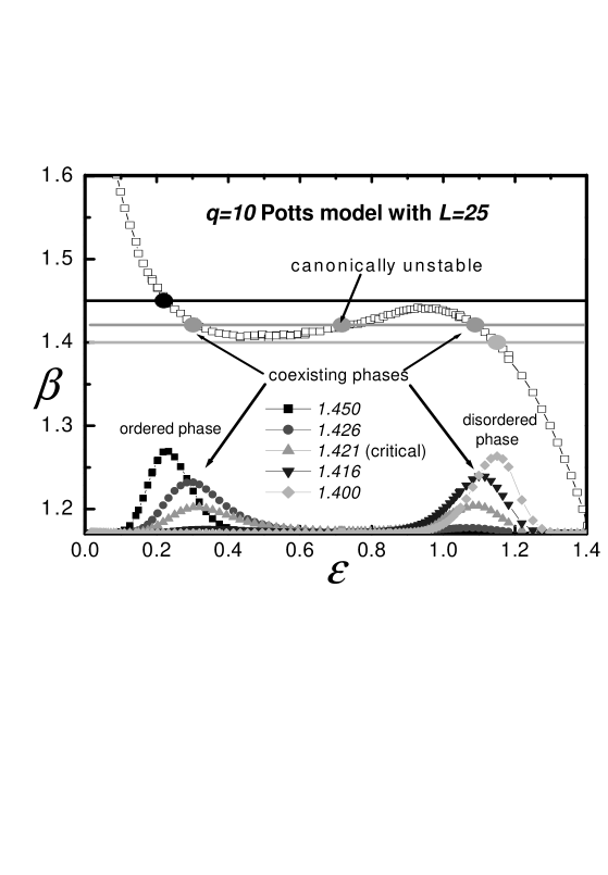
Figure 2: The energy distribution functions within the canonical ensemble, obtained from Eq.(7) by using $\Omega\left(E\right)$ estimated from Monte Carlo calculations (see sec. 3.1 below), indicate the occurrence of phase coexistence phenomenon in the $q=10$ states Potts model on the square lattice $N=L\times L$ with periodic boundary conditions ($\varepsilon=E/N$). Notice that the microcanonical states with negative heat capacities are practically inaccessible by using a thermostat with constant temperature, since these macrostates are canonically unstable.

The close relation between macrostates with negative heat capacities and first-order phase transitions in finite short-range interacting systems clarifies that such an ”anomalous” behavior is far from an unusual feature within the thermostatistical description, including also all those systems which have been traditionally considered within the standard Thermodynamics. The anomalous character of such macrostates reflects that they are physically admissible within the microcanonical description, while they are thermodynamically unstable within the canonical description; indicating thus the inequivalence of these statistical ensembles for finite systems.

As already evidenced, macrostates with $C<0$ do not receive a correct treatment by the fluctuation relations derived from the usual equilibrium situations of the standard Statistical Mechanics and Thermodynamics: in fact, the condition $C<0$ in Eq.(2) cannot be realized in a canonical description, where $\beta=$ constant, or within a microcanonical framework, where $E=$ constant so $\delta E$ vanishes. Precisely, the fundamental aim of this work is to obtain a suitable generalization of thermodynamic relation (2) in which accounts for appropriately the existence of macrostates with $C<0$.

The generalized fluctuation relation resulting from the present analysis points out the role of macrostates with $C<0$ in the experimental determination of the microcanonical caloric curve (which implies a simultaneous measurement of the temperature and energy of a given system), contributing in this way to a re-examination of an old question of the Thermo-Statistics Theory: Could it be possible the existence of certain kind of complementarity between the energy and the temperature? Such an idea was suggested by Bohr and Heisenberg in the early days of the Quantum Mechanics [17], and so far, it have not received a general consensus in the scientific literature [18].

This paper is organized into sections, as follows: First, in section 2, we introduce concepts like the generalized thermostat, effective inverse temperature and fluctuation in the Gaussian approximation to derive our fundamental result, Eq.(33). Second, in section 3, we discuss some implications on themodynamic control and measurements. Furthermore,  we perform a generalization of this result, Eq.(52), which constitutes an ”uncertainty relation” in Thermodynamics. Finally, in section 4, we make some concluding remarks about several theoretical and practical implications of the present formalism.

2 Extending fluctuation relation

2.1 Generalized thermostat

Derivation of a generalized fluctuation relation (2) to deal with macrostates with $C<0$ demands to face the problem of the ensemble inequivalence, to do this, we need to start from a more general equilibrium situation of the kind ”system-surrounding”, where macrostates with negative heat capacities can be arisen as thermodynamically stable under the external influence imposed by the system surrounding.

In thermodynamic equilibrium, the underlying physical conditions of the natural environment lead to a situation that a given short-range interacting system obeys the Gibbs canonical ensemble (1). The natural environment is a good example of a Gibbs thermostat, since its heat capacity is so large that it can be considered to be infinite in every practical situation. According to Lynden-Bell in ref.[14], a system with a negative heat capacity $C_{1}<0$ can reach thermodynamic equilibrium with a second system with $C_{2}>0$ when $0<C_{2}<\left|C_{1}\right|$. Obviously, such a condition does not hold when the first system is under the influence of the natural environment, since $C_{2}\rightarrow\infty$, and therefore, it is not possible to access the macrostates with negative heat capacities. As a corollary of this reasoning, the direct observation of the macrostates with negative heat capacities of a given system demands that the external influence of the natural environment be suppressed. Thus, the system of interest can be isolated (microcanonical ensemble) or it can be under the influence of a second system that remains of finite size. The latter possibility allows to express the energy distribution function of the first subsystem as follows:

$$\rho\left(E_{1}\right)dE_{1}=\frac{1}{\Omega_{c}\left(E_{T}\right)}\Omega_{2}\left(E_{T}-E_{1}\right)\Omega_{1}\left(E_{1}\right)dE_{1},$$ (8)

where $\Omega_{c}\left(E_{T}\right)=\int_{0}^{E_{T}}\Omega_{2}\left(E_{T}-E_{1}\right)\Omega_{1}\left(E_{1}\right)dE_{1}$ and as before, $\Omega_{2}\left(E_{2}\right)$ is the state density of the second system acting as a ”finite thermostat”, and $E_{T}$ is the total energy of the closed system $E_{T}=E_{1}+E_{2}$.

After reading the analysis presented in the subsequent subsections, it can be realized that the consideration of the ansatz (8) is sufficient to arrive at a generalized expression of the fluctuation relation (2): a closed system composed of two independent finite subsystems with an additive total energy. However, such a physical picture is only admissible when these subsystems are coupled by the incidence of short-range interacting forces or when long-range forces are confined to each subsystem which, however, is in general nonphysical. Even in this case this assumption presupposes to dismiss the energy contribution involved in their mutual interactions $V_{int}$. Although this is a licit and useful approximation in standard applications of Statistical Mechanics and Thermodynamics, it may be unrealistic in the case of mesoscopic systems with short-range interactions, and worse, this approach is not applicable in the case of long-range interacting systems. The latter case constitutes a typical scenario where macrostates with negative heat capacities naturally appear. Obviously, the additivity of the total energy is no longer applicable since the interaction energy $V_{int}$ cannot be considered as a ”boundary effect” as in the case of large systems with short-range interactions, and often, separability of a closed system into several parts is a hypothesis that should be carefully applied [19].

Nevertheless, we can find some systems in Nature where it is still possible to assume certain separability of a closed system into subsystems despite the presence of long-range interactions. Good examples are galaxies and their clusters. Of course, we are unable to dismiss the interactional energy $V_{int}$ in this scenario, but it is reasonable to assume as a consequence of the separability that this energy contribution could be approximated by certain functional dependence of the internal energies of each subsystems, $V_{int}\simeq V_{int}\left(E_{1},E_{2}\right)$. Thus, the usual additivity of the total energy $E_{T}$ could be substituted by the following ansatz:

$$E_{T}=\Phi\left(E_{1},E_{2}\right)\simeq E_{1}+E_{2}+V_{int}\left(E_{1},E_{2}\right).$$ (9)

The number of macrostates of the whole system $\Omega_{c}\left(E_{T}\right)$ is given by:

$$\Omega_{c}\left(E_{T}\right)=\int\delta\left[E_{T}-\Phi\left(E_{1},E_{2}\right)\right]\Omega_{1}\left(E_{1}\right)\Omega_{2}\left(E_{2}\right)dE_{1}dE_{2},$$ (10)

which allows to express the energy distribution of the first subsystem as follows:

$$\rho\left(E_{1};E_{T}\right)dE_{1}=\omega\left(E_{1};E_{T}\right)\Omega_{1}\left(E_{1}\right)dE_{1},$$ (11)

and the probabilistic weight $\omega\left(E_{1};E_{T}\right)$ by:

$$\omega\left(E_{1};E_{T}\right)=\frac{1}{\Omega_{c}\left(E_{T}\right)}\int\delta\left[E_{T}-\Phi\left(E_{1},E_{2}\right)\right]\Omega_{2}\left(E_{2}\right)dE_{2}.$$ (12)

Eq.(11) constitutes a more general expression than Eq.(8), providing a better treatment for a nonlinear energy interchange between the subsystems as a consequence of the nonadditivity of the total energy ($\Delta E_{1}\not=-\Delta E_{2}$). This kind of consideration could be applicable to both: the case of large systems with long-range interactions and mesoscopic systems with short-range interactions.

Previous discussions have suggested that a general way to account for the energy distribution function $\rho\left(E\right)dE$, which is associated to a general ”system-surrounding” equilibrium situation, is provided by the ansatz:

$$\rho\left(E\right)dE=\omega\left(E\right)\Omega\left(E\right)dE,$$ (13)

where $\Omega\left(E\right)$ represents the state density of the system with internal energy $E$, and $\omega\left(E\right)$, a generic probabilistic weight characterizing the energetic interchange of this system with its surrounding. The above hypothesis is very economical since it demands merely: (1) the existence of some kind of separability between the system and its surrounding, (2) and those all external influences on the system are fully described by the probabilistic weight $\omega\left(E\right)$. In this work, we are admitting the validity of Eq.(13) without mattering the internal structure of the surrounding, and even, the features of its internal equilibrium conditions. This last idea is very important and deserves to be clarified.

It is almost a rule that a large system with long-range interactions, initially far from the equilibrium, reaches rapidly a metastable equilibrium spending a long time in it [9]. If this is the case, the energy interchange of this large system acting as ”surrounding” of another system cannot be dealt by the expressions (8) or (11). However, this metastability does not forbid the applicability of the ansatz (13) in many physical situations. For example, it is well known that the collisionless dynamics of astrophysical systems leads to a metastable state where the one-particle distribution function $f\left(q,p\right)$ depends only on the particle energy $\varepsilon\left(q,p\right)=\frac{1}{2m}p^{2}+m\varphi\left(q\right)$, where $f\left(q,p\right)=f\left[\varepsilon\left(q,p\right)\right]$, whose mathematical form is not Boltzmannian and it is determined from the initial conditions of dynamics [20]. Since the macroscopic behavior of the system in this metastable state is also ruled by its energy, we can expect that this physical quantity also rules its interaction with other systems. The admittance of the validity of the ansatz (13) for systems in metastable conditions accounts for the claims of some recent authors about the existence of non-Boltzmannian energy distribution functions outside the equilibrium, overall, in systems with a complex microscopic dynamics, e.g.: astrophysical systems [20] and turbulent fluids [21]. A unifying framework for many of  these distribution functions is provided by the so-called ”Superstatistics”, a theory recently proposed by C. Beck and E.G.D Cohen [22], where the presence of a non-Boltzmannian weight $\omega\left(E\right)$ seems to be originated from an effective incidence of a fluctuating inverse temperature $\beta$ at the microscopic level (e.g. on a Brownian particle) obeying the distribution function $f\left(\beta\right)$ as follows:

$$\omega\left(E\right)=\int\exp\left(-\beta E\right)f\left(\beta\right)d\beta.$$ (14)

Since the microscopic origin and the specific mathematical form of the probabilistic weight $\omega\left(E\right)$ are arbitrary, it is expected that the conclusions, which are derived from the ansatz (13), may be applicable to a wide range of equilibrium or meta-equilibrium situations. In this formula, $\omega\left(E\right)$ constitutes a generic extension of the usual canonical weight:

$$\omega_{c}\left(E;\beta\right)=C\exp\left(-\beta E\right),$$ (15)

which rules the energy interchange of a Gibbs thermostat (a very large short-range interacting system). In an analogous way, we shall hereafter refer to the system surrounding associated with the weight $\omega\left(E\right)$ as a generalized thermostat. Let us now show that this generalized thermostat can be also characterized by certain effective inverse temperature $\beta_{\omega}$, which controls, as usual, the energetic interchange of this thermostat with the system under study.

2.2 Effective inverse temperature $\beta_{\omega}$

A straightforward way to arrive at this important thermodynamic quantity is by using the probabilistic weight $\omega\left(E\right)$ in the Metropolis Monte Carlo simulation of the system dynamics in this equilibrium condition. The acceptance probability for a Metropolis move $p\left(\left.E\right|E+\Delta E\right)$ is given by:

$$p\left(\left.E\right|E+\Delta E\right)=\min\left\{\frac{\omega\left(E+\Delta E\right)}{\omega\left(E\right)},1\right\}.$$ (16)

By assuming that the system size is large enough, consequently, the amount of energy $\left|\Delta E\right|\ll\left|E\right|$, we are able to introduce the approximation:

$$\ln\frac{\omega\left(E+\Delta E\right)}{\omega\left(E\right)}\simeq\frac{\partial\ln\omega\left(E\right)}{\partial E}\Delta E,$$ (17)

and rephrase the acceptance probability (16) as follows:

$$p\left(\left.E\right|E+\Delta E\right)\simeq\min\left\{\exp\left[-\beta_{\omega}\left(E\right)\Delta E\right],1\right\}.$$ (18)

The evident analogy of this last results with the canonical case allows to define the quantity $\beta_{\omega}\left(E\right)$

$$\beta_{\omega}\left(E\right)=-\frac{\partial\ln\omega\left(E\right)}{\partial E}$$ (19)

as the effective inverse temperature of the generalized thermostat.

It is possible to verify that this definition is not arbitrary. Besides the obvious case of the canonical weight (15) where $\beta_{\omega}\left(E\right)\$is the inverse temperature of the Gibbs thermostat, $\beta_{\omega}\left(E\right)\equiv\beta$, the present definition drops to the usual microcanonical inverse temperature of the system acting as a ”finite thermostat” in Eq.(8), where $\omega\left(E\right)=\Omega_{2}\left(E_{2}\right)/\Omega\left(E_{T}\right)$ and $\beta_{\omega}\left(E\right)\equiv\beta_{2}\left(E_{2}\right)=\partial S_{2}\left(E_{2}\right)/\partial E_{2}$, being $S_{2}\left(E_{2}\right)=\ln\left[\Omega_{2}\left(E_{2}\right)\delta E_{0}\right]$ and $E_{2}=E_{T}-E$.

This inverse temperature is ”effective” because it is not always equivalent to the ordinary interpretation of this concept in the standard Statistical Mechanics. In order to verify this fact, let us consider the equilibrium situation accounted for by Eq.(11). The internal energy of the second subsystem $E_{2}$ can be expressed as follows:

$$E_{2}=E_{T}-E_{1}-V_{int}\left(E_{1},E_{2}\right),$$ (20)

where the recursive substitution of this last equation in $V_{int}\left(E_{1},E_{2}\right)$ leads to the certain nonlinear dependence of $E_{2}$ on the internal energy of the first subsystem $E_{1}$:

$$E_{2}=E_{2}\left(E_{1}\right)\equiv E_{T}-\Theta\left(E_{1};E_{T}\right).$$ (21)

Thus, the probabilistic weight of Eq.(12) is similar to the case of the ”finite thermostat”:

$$\omega\left(E_{1};E_{T}\right)=\frac{\Omega_{2}\left[E_{2}\left(E_{1}\right)\right]}{\Omega\left(E\right)},$$ (22)

but the effective inverse temperature $\beta_{\omega}$ is given by:

$$\beta_{\omega}\left(E_{1}\right)=\frac{\partial S_{2}\left(E_{2}\right)}{\partial E_{2}}\nu\left(E_{1}\right),$$ (23)

where the factor $\nu\left(E_{1}\right)=-\partial E_{2}/\partial E_{1}=\partial\Theta\left(E_{1};E_{T}\right)/\partial E_{1}\not=1$ accounts for the existence of a nonlinear energy interchange as a consequence of the nonadditivity of the total energy. It is remarkable that the ”effective inverse temperature” of a very large system surrounding depends on the internal energy $E_{1}$ despite its ”microcanonical inverse temperature” $\beta_{2}=\partial S_{2}/\partial E_{2}$ remains practically unaltered by the underlying energy interchange, as in the case of the Gibbs thermostat.

The physical meaning of the effective inverse temperature $\beta_{\omega}$ is even more unclear in the case where the probabilistic weight $\omega\left(E\right)$ is associated with a system surrounding in a metastable equilibrium. Obviously, this kind of inverse temperature has nothing to do with the inverse temperature $\beta$ of the integral representation (14) of the Superstatistics formalism: while a whole set of values of $\beta$ for each energy $E$ exists, there is only one value of $\beta_{\omega}$ for each value of $E$. The importance of this new concept relies on the possibility to consider a wide class of equilibrium or meta-equilibrium situations in a unifying framework where it could be possible to extend the validity of some known thermostatistical results.

A fundamental identity is the condition of thermal equilibrium. This condition commonly follows from the analysis of  the most probable macrostate $\bar{E}$:

$$\max_{\bar{E}}\left\{\omega\left(E\right)\Omega\left(E\right)\right\}$$ (24)

which leads directly to the stationary equation:

$$\beta_{\omega}\left(\bar{E}\right)=\beta_{s}\left(\bar{E}\right),$$ (25)

where $\beta_{s}\left(E\right)$ is just the microcanonical inverse temperature of the system:

$$\beta_{s}\left(E\right)=\frac{\partial S\left(E\right)}{\partial E},$$ (26)

where, as in the introductory section, we take $S\left(E\right)=\ln W(E)$. We have demonstrated that the quantity $\beta_{\omega}$ also obeys the ordinary form of the Zeroth Principle of Thermodynamics . By analyzing the expression of $\beta_{\omega}$ shown in Eq.(23) associated with the equilibrium between two separable subsystems with a nonadditive total energy, Eq.(9), we notice that it is precisely $\beta_{\omega}$, and not $\beta_{2}$, which becomes equal to microcanonical inverse temperature of the first subsystem $\beta_{1}$ during the thermal equilibrium, $\beta_{\omega}=\beta_{1}\Rightarrow\beta_{2}\not=\beta_{1}$. This result is essentially the same as the one presented by Johal in the ref.[23].

Let us now summarize the fundamental properties of the effective inverse temperature $\beta_{\omega}$:

A.

It characterizes the energy interchange ”system-surrounding” during the equilibrium, in accordance with Eq.(18).

B.

This concept permits to extend the thermal equilibrium condition, Eq.(25), to a wide class of physical situations.

C.

In general, this thermodynamical quantity depends on the internal energy of the system $E$, $\beta_{\omega}\left(E\right)$.

Properties A and B correspond to the ordinary physical notion of temperature. A new remarkable property is the general dependence of $\beta_{\omega}$ on the internal energy $E$  of the system (the property C). This fact indicates clearly that the underlying energy interchange not only imposes fluctuations on the internal energy $E$, but also provokes the existence of correlated fluctuations between the internal energy $E$ and the effective inverse temperature of the thermostat $\beta_{\omega}$, $\left\langle\delta\beta_{\omega}\delta E\right\rangle\not=0$.  This simple property has been systematically disregarded by the use of the Gibbs canonical ensemble in standard Statistical Mechanics. We shall show in the next subsection that the property C is precisely the fundamental key for arriving at a suitable generalization of the fluctuation relation (2).

Before the end of this subsection, it is important to remark that the probabilistic weight:

$$\omega_{m}\left(E;E_{0}\right)=C\delta\left(E-E_{0}\right),$$ (27)

which is associated with the energetic isolation or the microcanonical ensemble, can be also considered as a limiting case of a generalized thermostat. The application of the definition (19) leads to an indeterminate value of $\beta_{\omega}$:

$$\beta_{\omega}\left(E\right)=-\frac{\partial}{\partial E}\ln\delta\left(E-E_{0}\right)=indeterminate,$$ (28)

which means that the thermostat inverse temperature $\beta_{\omega}$ admits any value when the energy of the system is fixed at $E_{0}$. This idea is schematically illustrated in FIG.3.

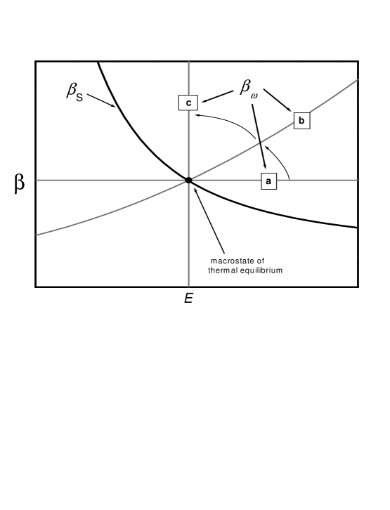
Figure 3: Typical behavior of the effective inverse temperature $\beta_{\omega}$ is depicted for: a) $\beta_{\omega}$ fixed for all values of $E$ (canonical ensemble), b) an arbitrary dependence $\beta_{\omega}\left(E\right)$ (generalized thermostat), and c) $E$ fixed for all values of $\beta_{\omega}$ (microcanonical ensemble). The black thick point represents the macrostate of thermal equilibrium where $\beta_{\omega}=\beta_{s}$, and $\beta_{s}\left(E\right)=\partial S\left(E\right)/\partial E$, the microcanonical inverse temperature of the system.

2.3 Fluctuations in the Gaussian approximation

We shall suppose in the present analysis that the system and bath are large enough in order to support a Gaussian approximation of the energy fluctuations around the most probable macrostate $\bar{E}$. In addition, we also assume that the energy dependence of the effective inverse temperature $\beta_{\omega}\left(E\right)$ allows for the existence of only one intersection point $\bar{E}$ with the microcanonical caloric curve of the system $\beta_{s}\left(E\right)$ in the thermal equilibrium condition (25). This latter requirement is just the condition of ensemble equivalence. The average square dispersion of the internal energy $\left\langle\delta E^{2}\right\rangle$:

$$\left\langle\delta E^{2}\right\rangle=\int\left(E-\bar{E}\right)^{2}\omega\left(E\right)\Omega\left(E\right)dE$$ (29)

can be estimated as follows:

$$\left\langle\delta E^{2}\right\rangle^{-1}=-\frac{\partial^{2}}{\partial E^{2}}\left\{\ln\omega\left(\bar{E}\right)+S\left(\bar{E}\right)\right\}.$$ (30)

The fluctuation $\delta\beta_{\omega}=\beta_{\omega}\left(E\right)-\beta_{\omega}\left(\bar{E}\right)$ of the effective inverse temperature can be related to the fluctuation $\delta E$ of the internal energy of the system:

$$\delta\beta_{\omega}=-\frac{\partial^{2}\ln\omega\left(\bar{E}\right)}{\partial E^{2}}\delta E.$$ (31)

If we rewrite Eq.(30) in the following manner,

$$-\frac{\partial^{2}\ln\omega\left(\bar{E}\right)}{\partial E^{2}}=\left\langle\delta E^{2}\right\rangle^{-1}+\frac{\partial^{2}S\left(\bar{E}\right)}{\partial E^{2}},$$ (32)

and combine Eq.(31) and (32), we arrive at the correlation between the effective inverse temperatures of the generalized thermostat and the internal energy of the system as follows:

$$\left\langle\delta\beta_{\omega}\delta E\right\rangle=1+\frac{\partial^{2}S\left(\bar{E}\right)}{\partial E^{2}}\left\langle\delta E^{2}\right\rangle.$$ (33)

This latter identity is a generalized expression of the fluctuation relation (2). This fact can be noticed by rephrasing (33) as follows:

$$C=\beta^{2}\left\langle\delta E^{2}\right\rangle+C\left\langle\delta\beta_{\omega}\delta E\right\rangle$$ (34)

by using the microcanonical definition of the heat capacity, Eq.(4), being $\beta=\beta_{s}\left(\bar{E}\right)$.

3 Discussions

We remark that the fluctuation relation (33) accounts for the specific mathematical form of the probabilistic weight $\omega\left(E\right)$ in an implicit way throughout the effective inverse temperature $\beta_{\omega}$. Once more, this result evidences the fact that the system-surrounding energy interchange is effectively controlled by $\beta_{\omega}$. The imposition of the restriction $\delta\beta_{\omega}=0$ associated with the Gibbs canonical ensemble (1) into Eq.(34) leads to the usual identity $C=\beta^{2}\left\langle\delta E^{2}\right\rangle$. However, the restriction $\delta\beta_{\omega}=0$ is not compatible with the existence of energetic regions with negative heat capacities $C<0$. Since the microcanonical entropy is locally convex $\partial^{2}S\left(\bar{E}\right)/\partial E^{2}>0$ in such anomalous regions, the identity (33) leads here to the inequality:

$$\left\langle\delta\beta_{\omega}\delta E\right\rangle>1.$$ (35)

This means that any attempt to impose the canonical condition $\delta\beta_{\omega}\rightarrow 0$, within regions with $C<0$, leads to the occurrence of very large energy fluctuations $\delta E\rightarrow\infty$, and conversely, any attempt to impose the microcanonical condition $\delta E\rightarrow 0$ is accompanied by very large fluctuations of the effective inverse temperature of the system surrounding $\delta\beta_{\omega}\rightarrow\infty$. Remarkably, this behavior suggests the existence of some kind of complementarity between the internal energy $E$ and the effective inverse temperature $\beta_{\omega}$ of the surrounding, which is quite analogous to the complementarity between a coordinate $q$ and its conjugated momentum $p$ in Quantum Mechanics! As well, the divergence $\delta\beta_{\omega}\rightarrow\infty$ when $\delta E\rightarrow 0$ is not only applicable to regions where $C<0$: any attempt to reduce the energy fluctuations to zero, $\delta E\rightarrow 0$, in Eq.(33) for any fixed $\bar{E}$ leads to the following result:

$$\lim_{\delta E\rightarrow 0}\left\langle\delta\beta_{\omega}\delta E\right\rangle=1,$$ (36)

indicating thus the divergence of the effective inverse temperature fluctuations $\delta\beta_{\omega}\rightarrow\infty$ at this limit. The present results allow to conclude:

(i)

While macrostates with $C>0$ are accessible within the canonical ensemble, where takes place the restriction $\delta\beta_{\omega}=0$, the anomalous macrostates where $C<0$ can be only accessed when $\delta\beta_{\omega}\not=0$, that is, by using a generalized thermostat whose energy dependence of its effective inverse temperature $\beta_{\omega}\left(E\right)$ ensures the validity of the inequality (35).

(ii)

The total energy $E$ of the system and the effective inverse temperature of the generalized thermostat $\beta_{\omega}$ behave as complementary thermodynamic quantities within the regions with $C<0$.

(iii)

The imposition of the microcanonical restriction $\delta E\rightarrow 0$ leads at any internal energy $E$ to an indetermination of the effective inverse temperature of the system surrounding $\delta\beta_{\omega}\rightarrow\infty$ as a consequence of the suppression of the underlying energetic interchange.

A deeper understanding of the physical meaning of the previous conclusions is reached by discussing their implications on the two standard ways where the external influence of the surrounding on the thermodynamic state of the system is used within the Thermodynamics:

• as a control apparatus (thermostat), or

• as a measure apparatus (thermometer).

3.1 Implications on the thermodynamic control

It is well-known that the (inverse) temperature is, in general, a good control parameter for the internal energy of a system: the contact of a thermostat with a given constant value $\beta$ leads to the existence of small fluctuations of the internal energy $\delta E\propto\sqrt{N}$, where $N$ is the system size. The remarkable exception is that during the first-order phase transitions. Here, a small variation on $\beta$ is able to provoke a sudden change in the expectation value of the internal energy $\left\langle E\right\rangle$ of the system due to the multimodal character of the energy distribution function in the neighborhood of the critical inverse temperature $\beta_{c}$, which provokes very large energy fluctuations $\delta E\propto N$. This physical situation was already illustrated in FIG.2 of the introductory section for the case of the thermodynamical description of the $q=10$ states Potts model on the square lattice (6), where the origin of this anomaly relies on the existence of inaccessible or unstable energetic regions with $C<0$.

From the perspective of the thermodynamic control, the fluctuation relation of Eq.(33) describes the necessary conditions where the external influence imposed by the surrounding ensures the thermodynamic stability of the system, allowing thus an effective control of the internal energy $E$ of the controlled system. The term ”effective control” means that the internal energy of the system is preserved until the precision of small fluctuations around the average value $\bar{E}$. This kind of fluctuating behavior is ensured by the ensemble equivalence or the existence of only one sharp peak in the energy distribution function $\rho\left(E\right)dE$, which is mathematically expressed by the existence of only one intersection point $\bar{E}$ in the condition of thermal equilibrium (25).

The Conclusion (i) claims basically that macrostates with $C<0$ can be forced to be thermodynamically stable or accessible by using a generalized thermostat with an appropriate energy dependence in its effective inverse temperature $\beta_{\omega}\left(E\right)$. This situation is clearly illustrated in FIG.4, where this particular external influence has automatically eliminated the bimodal character of the energy distribution function of the $q=10$ states Potts model in the neighborhood of the critical temperature shown in FIG.2.

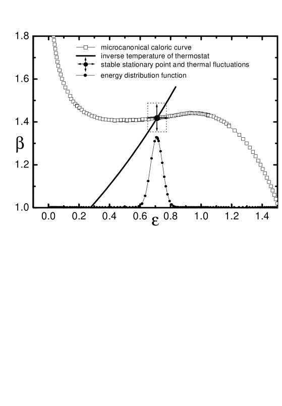
Figure 4: Metropolis Monte Carlo calculations for the 10-state Potts model by using Eq.(18). Consideration of a thermostat with a variable inverse temperature $\beta_{\omega}\left(E\right)$ can ensure the existence of a unique stable stationary point of the microcanonical caloric curve $\beta_{s}\left(E\right)$ where $\beta_{\omega}=\beta_{s}$, in this way the system can be forced to access its anomalous macrostates with $C<0$, and at the same time, to eliminate the bimodal character of the energy distribution function in the neighborhood of the critical inverse temperature $\beta_{c}$.

The divergence $\delta E\rightarrow\infty$ when $\delta\beta_{\omega}\rightarrow 0$ within the region with $C<0$ indicated in the Conclusion (ii) accounts for the well-known fact that such macrostates turn unstable or inaccessible within the canonical description. This divergence is just a consequence of the Gaussian approximation which has been employed to obtain the fluctuation relation (33), since the energy fluctuations are actually on the order of the system size, $\delta E\propto N$, which diverge only in the thermodynamic limit $N\rightarrow\infty$. The Conclusion (iii) is just the mathematical result previously obtained in Eq.(28) and illustrated in FIG.3. Conveniently, the practical implications of this result will be discussed in the next subsection.

As already shown, the consideration of a generalized thermostat with an appropriate energy dependence of its effective inverse temperature $\beta_{\omega}\left(E\right)$ is a simple but an effective consideration to overcome the difficulties associated with the existence of macrostates with $C<0$. In principle, the practical implementation of the present ideas should lead to the development of some experimental techniques which could be particularly useful to deal with thermodynamical description of mesoscopic systems which are now of interest of Nanosciences, and where the presence of macrostates with $C<0$ is not unusual.

Another important framework of applications is to develop more efficient Monte Carlo methods to deal with the difficulties associated to the presence of first-order phase transitions [24]. A simple and general way to account for the presence of a generalized thermostat with a given effective inverse temperature $\beta_{\omega}\left(E\right)$ is by using the Metropolis method based on the acceptance probability of Eq.(18). In fact, the microcanonical caloric curve $\beta_{s}\left(\varepsilon\right)$ of the $q=10$ states Potts model shown in FIG.2 and FIG.4 were obtained using this methodology by calculating the averages $\left\langle\varepsilon\right\rangle$ and $\left\langle\beta_{\omega}\right\rangle$, where the validity of the Gaussian approximation for $N$ large enough and the condition of thermal equilibrium (25) ensure the applicability of the relations:

$$\bar{\varepsilon}=\left\langle\varepsilon\right\rangle~{}~{}and~{}~{}\beta_{s}\left(\bar{\varepsilon}\right)=\left\langle\beta_{\omega}\right\rangle.$$ (37)

Numerical results derived from this algorithm agree very well with the ones obtained using other Monte Carlo methods [25].

The idea of using the generalized thermostat with an appropriate effective inverse temperature $\beta_{\omega}\left(E\right)$ can be easily extended to other Monte Carlo methods based on the Gibbs canonical ensemble. A specific example is the enhancement of the well-known Swendsen-Wang (SW) cluster algorithm [16], which suffers from the supercritical slowing down in its application to the $q=10$ states Potts model on the square lattice and is unable to capture the $C<0$ regime of the microcanonical caloric curve. The thermostat inverse temperature $\beta$ enters into this method by the probability for the cluster formation $p\left(\beta\right)=1-\exp\left(-\beta\right)$, which is used to generate a new system configuration $X$. While the parameter $\beta$ remains constant in the original SW algorithm, our modification consists in the substitution of this parameter by the effective inverse temperature of the generalized thermostat $\beta_{\omega}$, which is redefined in each Monte Carlo step, $\beta_{\omega}^{i}\rightarrow\beta_{\omega}^{i+1}$. The parameter $\beta_{\omega}^{i+1}$ used to generate the configuration $X^{i+1}$ takes the value of the effective inverse temperature corresponding to the total energy $E_{i}=H_{N}\left(X^{i}\right)$ of the previous system configuration $X^{i}$, $\beta_{\omega}^{i}=\beta_{\omega}\left(E_{i}\right)$. Here, $H_{N}$ is the Hamiltonian of Eq.(6) and $X=\left\{\sigma_{k}\right\}$ the spin variables. The microcanonical caloric curve is determined by using the same relations (37) of the Metropolis method explained before. In FIG.5 a comparative study among the ordinary SW method (CE) and the Metropolis and SW methods with an appropriate effective inverse temperature (GCE) is depicted. The agreement between these last Monte Carlo algorithms and their advantages over the first method is remarkable. As clearly evidenced, the present ideas support the development of an alternative framework of the well-known multicanonical Monte Carlo methods [24]. As in FIG.3 as Monte Carlo calculations shown in FIG.4 and FIG.5, the following effective inverse temperature:

$$\beta_{\omega}\left(E\right)=\eta\exp\left[\lambda\left(E-E_{0}\right)/N\right]$$ (38)

was assumed, where $\eta$ and $\lambda$ are two real positive parameters controlling the horizontal position and the inclination of this dependence respectively. The value $\lambda=0$ corresponds to the canonical ensemble (1), while $\lambda\rightarrow+\infty$ corresponds to the microcanonical ensemble (27). More details of these calculations can be found in the ref.[26].

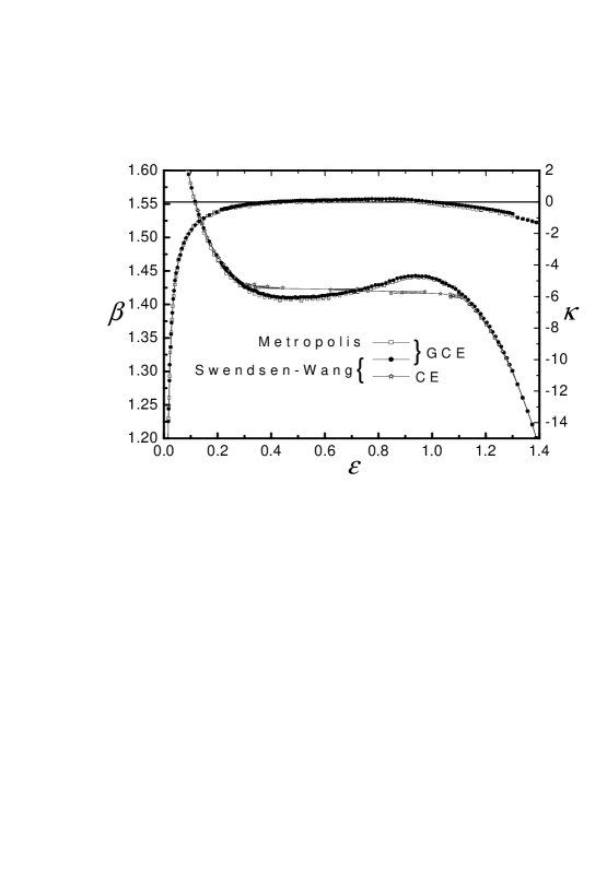
Figure 5: The ordinary Swendsen-Wang cluster algorithm (CE) is unable to account for the $C<0$ regime of the microcanonical caloric curve $\beta_{s}\left(\varepsilon\right)=\partial s\left(\varepsilon\right)/\partial\varepsilon$ of the $q=10$ states Potts model on the square lattice as shown here by our Monte Carlo calculations. This difficulty is overcome by the Metropolis algorithm and the Swendsen-Wang cluster algorithm based on the use of an effective inverse temperature $\beta_{\omega}$ (GCE), where one can note a remarkable agreement between these algorithms. In addition, we also show here the energy per particle $\varepsilon$ dependence of the second derivative of the entropy per particle, $\kappa\left(\varepsilon\right)=\partial^{2}s\left(\varepsilon\right)/\partial\varepsilon^{2}$, which has been obtained from the fluctuation relation (33) by calculating the fluctuations quantities $\left\langle\delta\varepsilon^{2}\right\rangle$ and $\left\langle\delta\beta_{\omega}\delta\varepsilon\right\rangle$. This dependence clearly evidence the existence of an anomalous region where $\kappa\left(\varepsilon\right)>0\Leftrightarrow C<0$.

3.2 Implications on the thermodynamic measurements: An uncertainty relation?

Bohr and Heisenberg suggested in the past that the thermodynamic quantities of temperature and energy are complementary in the same way as the position and the momentum are related in Quantum Mechanics [17]. Roughly speaking their idea was that a definite temperature can be attributed to a system only if it is submerged in a heat bath (Gibbs thermostat). Energy fluctuations are unavoidable. On the contrary, a definite energy can be only assigned to systems in thermal isolation, thus excluding the simultaneous determination of its temperature. Dimensional considerations suggest the existence of the following relation:

$$\delta\beta\delta E\geq 1.$$ (39)

However, these ideas have not reached a general consensus in the literature [18].One objection is that the mathematical structure of Quantum theories is radically different from that of classical physical theories, so that, there are no noncommuting observables in Thermodynamics. Interestingly, the result expressed in Eq.(35) is quite analogous to the uncertainty relation (39).

Before analyzing the implications of the fluctuation relation (33) in the thermodynamic measurements, it is important to revise the concept of temperature of a system. In the Bohr and Heisenberg arguments explained above, as well as in the works of some other authors like the Landau (see last paragraph of pag. 343 in ref.[1]) and Mandelbrot [27], a system has a definite temperature when it is put into contact with a Gibbs thermostat. In this viewpoint, the concept of the temperature of an isolated system is unclear. We think this is a misunderstanding, since the inverse temperature $\beta$ that enters in the Gibbs canonical ensemble (1) is just the microcanonical inverse temperature of the Gibbs thermostat (th), $\beta=\partial S_{th}/\partial E_{th}$. This quantity does not properly characterize the thermodynamic state of the system, but instead it characterizes the thermodynamic state of the thermostat and its thermal influence on the system. Hereafter, we refer to the inverse temperature of a system defined as its microcanonical inverse temperature $\beta_{s}=\partial S\left(E\right)/\partial E$. From this perspective, the temperature of an isolated system is a well-defined quantity and does not undergo fluctuations, $\delta E=0\Rightarrow\delta\beta_{s}=0$.

Although it is possible to obtain the system temperature at a given energy by calculating the Boltzmann entropy $S\left(E\right)$, the practical determination of the temperature is always imprecise. The energy is a quantity with a mechanical significance, and it can be determined by performing only one instantaneous measurement on an isolated system. The temperature is a quantity with a thermo-statistical significance, whose determination demands to appeal to the concept of statistical ensemble. For example, it is derived from a statistics of measurements or temporal averages of certain physical observables with a mechanical significance usually referred to thermometric quantities (e.g.: the length of a mercury column, an electric signal, the pressure of an ideal gas, the average form of a particles distribution function, etc.). In practice, the temperature $\beta_{s}$ of a given system is indirectly measured from its interaction with another system (usually smaller than the system under study and referred to thermometer (th)), whose internal dependence of its temperature $\beta_{th}$ on a thermometric quantity is previously known. The fundamental key supporting this procedure is precisely the condition of thermal equilibrium:

$$\beta_{s}=\beta_{th}.$$ (40)

In our approach, the surrounding can be also used as a measurement apparatus (thermometer), so that, the quantity $\beta_{th}$ is just the effective inverse temperature $\beta_{\omega}$. It is possible to realize that the generalized thermostat used in the previous Monte Carlo calculations has the dual role: to be a control and a measure apparatus at the same time. In fact, the energy dependence of the microcanonical inverse temperature $\beta_{s}$ of the Potts model is a priori unknown, and, we estimate it through the effective inverse temperature of the generalized thermostat $\beta_{\omega}$ via the condition of thermal equilibrium in Eq.(37). This kind of computational procedure exhibits essential features of a real determination of the energy-temperature dependence (caloric curve).

Despite the apparent simplicity, the determination of the energy-temperature dependence of a system by using this procedure is rather complex, which is evidenced from the two factors affecting its precision:

• This measurement process necessarily involves a perturbation on the thermodynamic state of the system.

• The interaction also affects the thermodynamic state of the thermometer in an uncontrollable stochastic way, which provokes the existence of errors in the determination of the effective inverse temperature $\beta_{\omega}$ used to estimate $\beta_{s}$ via the condition of thermal equilibrium.

It is possible to see in the Conclusions (ii) and (iii) that the precision factors A and B are rather complementary. The error type A can be characterized in terms of the system energy fluctuations $\delta E$, since the inverse temperature fluctuation $\delta\beta_{s}$ is directly correlated with $\delta E$. The error type B is characterized in terms of the effective inverse temperature fluctuations $\delta\beta_{\omega}$, which may also depend on $\delta E$, but in an indirect way. According to the Conclusion (iii), any attempt to reduce the perturbation of the system to zero, $\delta E\rightarrow 0$, (the error type A) leads to a progressive increasing of the error type B, $\delta\beta_{\omega}\rightarrow\infty$, which affects the estimation of $\beta_{s}$ by using $\beta_{\omega}$. The error type B can reduce to zero $\delta\beta_{\omega}\rightarrow 0$ by imposing the conditions of the Gibbs canonical ensemble (1), which always involves certain perturbations of the system energy $\delta E\not=0$ (error type A). This perturbation is relatively small when the system size is large enough and the heat capacity of the system is positive $C>0$. However, this situation changes radically when the macrostate of the system is characterized by a negative heat capacity $C<0$. According to the Conclusion (ii), the reduction of the error type B to zero, $\delta\beta_{\omega}\rightarrow 0$, induces the thermodynamic instability of the macrostates with $C<0$ and leads to the existence of very large energy fluctuations $\delta E\rightarrow\infty$. In practice, we should admit the simultaneous existence of the errors type A and B, which can reasonably be small and unimportant, when the sizes of the system under study and the thermometer are large enough. However, such errors are much significant when the system size $N$ is small (in a system of few bodies or constituents) that the concept of system temperature becomes experimental unobservable, and therefore, physically meaningless.

As already evidenced, the fluctuation relation of Eq.(33) accounts in some way for the limit of precision for a determination of the energy-temperature dependence of a given system by using a measurement procedure based on thermal equilibrium with another system (thermometer). Although this qualitative behavior is quite close to the Bohr and Heisenberg intuitive idea of energy-temperature complementarity, the fluctuation relation (33) does not always support a complementary relationship between the system energy $E$ and the effective inverse temperature $\beta_{\omega}$ or the system energy $E$ and inverse temperature $\beta_{s}$. The reason is that the mathematical structure of Eq.(33) does not have the form of a complementary relation. Fortunately, this limitation is not difficult to overcome.

3.3 Generalization: The Quantum-Statistical Mechanics analogy

The derivation of the restricted fundamental result (33) relies on the Gaussian approximation. However, there is a simple way to overcome this difficulty. The inverse temperature fluctuation $\delta\beta_{s}$ can be expressed for small $\delta E$ in the following way:

$$\delta\beta_{s}=\frac{\partial^{2}S}{\partial E^{2}}\delta E;$$ (41)

therefore, the fluctuation relation (33) can be rephrased as follows:

$$\left\langle\delta\eta\delta E\right\rangle=1,$$ (42)

where $\eta$ is the difference between the effective inverse temperature of the generalized thermostat and the microcanonical inverse temperature of the system:

$$\eta=\beta_{\omega}-\beta_{s}.$$ (43)

The validity of result (42) does not depend on the Gaussian approximation. In order to show this, let us denote by $\rho\left(E\right)=\omega\left(E\right)\Omega\left(E\right)$ the energy distribution function of the ansatz (13). The distribution function $\rho\left(E\right)$ is not arbitrary. It obeys the following general mathematical conditions:

• Existence: The distribution function $\rho\left(E\right)$ is a nonnegative, bounded, and differentiable function on the set $\pi\subset R$ of all physically admissible energies $E$.

• Normalization: This function obeys the normalization condition:

  $$\int_{\pi}\rho\left(E\right)dE=1.$$ (44)

• Boundary conditions: This function vanishes together with its first derivative on boundary $\partial\pi$ of the set $\pi$:

  $$\forall E\in\partial\pi:\rho\left(E\right)=\frac{\partial}{\partial E}\rho\left(E\right)=0.$$ (45)

The key of the demonstration is the consideration of the following identity:

$$\left\{-\frac{\partial}{\partial E}\right\}\rho\left(E\right)=\eta\rho\left(E\right),$$ (46)

which allows to associate the quantity $\eta$ to an ”operator” $\hat{\eta}$:

$$\hat{\eta}=-\frac{\partial}{\partial E}.$$ (47)

By using the identity (46) as well as the properties (C2) and (C3) of the distribution function $\rho\left(E\right)$, it is easy to obtain the following results:

$$\left\langle\eta\right\rangle=\int_{\pi}\eta\rho\left(E\right)dE=\int_{\pi}\hat{\eta}\rho\left(E\right)dE=0,$$ (48)

$$\left\langle E\eta\right\rangle=\int_{\pi}E\eta\rho\left(E\right)dE=\int_{\pi}E\hat{\eta}\rho\left(E\right)dE=1.$$ (49)

The result (48) is just the condition of thermal equilibrium, Eq.(25). The fundamental result (42) is immediately obtained from Eq.(49) by operating as follows:

$$\left\langle\eta\right\rangle=0\Rightarrow\left\langle E\eta\right\rangle-\left\langle E\right\rangle\left\langle\eta\right\rangle\equiv\left\langle\delta E\delta\eta\right\rangle=1.$$ (50)

The result (42) can be rephrased one more time by using the well-known Schwarz inequality:

$$\left\langle\delta A^{2}\right\rangle\left\langle\delta B^{2}\right\rangle\geq\left\langle\delta A\delta B\right\rangle^{2}$$ (51)

arriving finally at a definitive result:

$$\Delta\eta\Delta E\geq 1,$$ (52)

where $\Delta\eta=\sqrt{\left\langle\delta\eta^{2}\right\rangle}$ and $\Delta E=\sqrt{\left\langle\delta E^{2}\right\rangle}$.

Undoubtedly, the expression (52) has the form of ”an uncertainty relation” that exhibits now a very general validity. It clarifies that the complementary relation actually exists for the system energy $E$ and the inverse temperature difference $\eta$ between the system and its surrounding (acting as a thermostat or a thermometer). Any attempt to perform an exact determination of the system temperature $\beta_{s}$ throughout the thermal equilibrium, $\Delta\eta\rightarrow 0$, involves a strong perturbation on the system energy $\Delta E\rightarrow\infty$, thus, $E$ becomes indeterminable; any attempt to reduce this perturbation to zero, $\Delta E\rightarrow 0$, makes impossible to determine the system inverse temperature $\beta_{s}$ by using the condition of thermal equilibrium since $\Delta\eta\rightarrow\infty$.

Remarkably, the above thermodynamic complementarity between $E$ and $\eta$ is quite analogous to the complementarity in Quantum theories. Contrary to what was preliminarily objected, this complementarity could be also supported in terms of the noncommutativity of mathematical operators $\hat{E}\equiv E$ and $\hat{\eta}\equiv-\partial_{E}$:

$$\left[\hat{E},\hat{\eta}\right]=1\Leftrightarrow\Delta\eta\Delta E\geq 1.$$ (53)

Thus, the relations of Eq.(53) can be considered the Statistical Mechanics counterpart of the familiar quantum relations:

$$\left[\hat{q},\hat{p}\right]=i\Leftrightarrow\Delta q\Delta p\geq 1,$$ (54)

where $\hslash\equiv 1$. The formal correspondence is: $q\sim E$ and $p\sim\eta$. This Quantum-Statistical Mechanics analogy can be also extended to the properties of the distribution functions: $\rho\left(q\right)=\left|\psi\left(q\right)\right|^{2}$ and $\rho\left(E\right)=\omega\left(E\right)\Omega\left(E\right)$, since the quantum distribution function $\rho\left(q\right)$ also obeys the properties (C1), (C2) and (C3). Demanding a little of imagination, the behavior of the energy distribution function in the neighborhood of the critical point illustrated in FIG.2 possesses a certain analogy with the tunneling of the distribution function $\rho\left(q\right)$ (a wave packet) throughout a classical barrier; that is, the phase coexistence phenomenon can be interpreted as a ”tunneling” of the energy distribution function $\rho\left(E\right)$ throughout the canonically inaccessible region.

Obviously, such a Quantum-Statistical Mechanics analogy should not be overestimated, although it is licit to recognize that it is very interesting: (1) Both are physical theories with a statistical mathematical apparatus; (2) While Quantum Mechanics is a theory hallmarked by the Ondulatory-Corpuscular dualism, Statistical Mechanics is also hallmarked by another kind of dualism since it works simultaneously with physical quantities with a purely mechanical significance (e.g.: energy) and physical quantities with a purely thermo-statistical significance (e.g.: inverse temperature); (3) Thermodynamics is the counterpart theory of Classical Mechanics: while Classical Mechanics assumes the simultaneous determination of position $q$ and momentum $p$ when $\hslash\rightarrow 0$, Thermodynamics assumes the simultaneous determination of the system energy $E$ and its temperature $\beta_{s}$ in the thermodynamic limit $1/N\rightarrow 0$.

Our approach to uncertainty relations in Thermodynamics constitutes an improvement of the works of Rosenfeld and Schölgl [28, 29], which have been also based on Fluctuation theory [1]. These authors derived their respective formulations from the consideration of a surrounding in the thermodynamics limit, and hence, this physical situation actually corresponds to the Gibbs canonical ensemble or in general the Boltzmann-Gibbs distribution [18]. Since this work hypothesis presupposes a concrete thermodynamic influence, an experimentalist has no free will to change the fluctuational behavior of the system in a given thermodynamic state.

This important limitation is overcome in our work: the fluctuational behavior of the system-surrounding equilibrium is modified by considering a different energy dependence of the effective inverse temperature $\beta_{\omega}\left(E\right)$, which presupposes to use a different experimental arrangement. In addition, it is not necessary to appeal to Statistical Inference theory to arrive at an uncertainty relation, as in the Mandelbrot development [30], which undergoes the same ”free will limitation” of the Rosenfeld and Schölgl works explained above since it is applicable only to the framework of the Gibbs canonical ensemble. Interestingly, no one of the above approaches says anything about the relevance of anomalous macrostates with $C<0$ on the practical determination of the system energy-temperature dependence.

4 Conclusions

In an attempt to establish an appropriate framework in order to deal with the existence of macrostates with negative heat capacities in terms of a fluctuation theory, we have introduced the concept of effective inverse temperature $\beta_{\omega}$, which characterizes the thermodynamic influence of the surrounding on the system under study, and specially, allows to extend the condition of thermal equilibrium to a wide class of equilibrium or meta-equilibrium situations. Precisely in terms of this quantity we arrive at a suitable generalization of the well-known canonical relation between the heat capacity and the energy fluctuation, $C=\beta^{2}\left\langle\delta E^{2}\right\rangle$. The new identity, Eq.(33), defines a criterion capable of detecting macrostates with negative heat capacities of the system under study through the correlated fluctuations of the effective inverse temperature $\beta_{\omega}$ of the surrounding (generalized thermostat) and the energy $E$ of the system itself. This last constitutes a novel kind of mechanics to perform a more effective thermodynamic control on those anomalous macrostates hidden behind the phenomenon of ensemble inequivalence, which inspires the developments of new experimental techniques of control to deal with the thermodynamic description for mesoscopic systems, like those which are now of interest in Nanosciences, as well as the introduction of new Monte Carlo methods to overcome the difficulties associated with the presence of first-order phase transitions.

We think that a significant aspect of this paper is to provide new physical arguments supporting the existence of a complementary relation, between the system energy and temperature, as postulated by Bohr and Heisenberg in the early days of the Quantum Mechanics. Both the fluctuation relation (33) and its generalization (52), which can be regarded as an uncertainty relation, impose limitations to the precise determination of the energy-temperature dependence (caloric curve) of the system under study by using a measurement procedure based on thermal equilibrium with another system (thermometer). While this limitation is unimportant in large enough systems, it discards the practical utility of some concepts of Thermodynamics in the context of systems with a small number of constituents. Surprisingly, these results suggest the existence of a remarkable analogy between the Statistical Mechanics and the Quantum Mechanics.

References

References

- [1] L. D. Landau and E. M. Lifshitz, Statistical Physics (Pergamon Press, London, 1980).
- [2] Moretto L G, Ghetti R, Phair L, Tso K, Wozniak GJ 1997 Phys. Rep. 287 250.
- [3] Ison M J, Chernomoretz A, Dorso C O 2004 Physica A 341 389.
- [4] D’Agostino M, Gulminelli F, Chomaz P, Bruno M, Cannata F, Bougault R, Gramegna F, Iori I, Le Neindre N, Margagliotti GV, Moroni A, Vannini G 2000 Phys. Lett. B 473 219.
- [5] Gross D H E and Madjet M E 1997 Z. Phys. B 104 521
- [6] Lynden-Bell D 1967 MNRAS 136 101.
- [7] Lynden-Bell D and Wood R 1968 MNRAS 138 495;
- [8] B. Einarsson 2004 Phys. Lett. A 332 335.
- [9] T. Dauxois, S. Ruffo, E. Arimondo, and M. Wilkens, Dynamics and Thermodynamics of Systems with Long Range Interactions (Springer, New York, 2002).
- [10] Thirring W 1972, Essays in Physics 4 125.
- [11] Antonov V A 1962 Vest. Leningr. Gos. Univ. 7 135.
- [12] Lynden-Bell D and Lynden-Bell R M 1977 MNRAS 181 405.
- [13] Padmanabhan T, Physics Reports 1990 188 285.
- [14] Lynden-Bell D 1999 Physica A 263 293.
- [15] Gross D H E 2001 Microcanonical thermodynamics: Phase transitions in Small systems,66 Lectures Notes in Physics, (World scientific, Singapore).
- [16] Wolff U 1989 Phys. Rev. Lett. 62 361.
- [17] Bohr N in: Collected Works, J. Kalckar, Ed. (North-Holland, Amsterdam, 1985), Vol. 6, pp. 316-330, 376-377.
- [18] Uffink J and van Lith J 1999, Thermodynamic Uncertainty Relations, Found. Phys. 29 655.
- [19] Landsberg P T 1991 Thermodynamics and Statistical Mechanics, (Dover).
- [20] Chavanis P H 2002 in: T. Dauxois, S. Ruffo, E. Arimondo, M. Wilkens (Eds.), Dynamics and Thermodynamics of Systems with Long Range Interactions, Lecture Notes in Physics, Springer; e-print (2002) [cond-mat/0212223].
- [21] Beck C 2001 Phys. Rev. Lett. 87 18061; Physica A 277 (2000) 115; Physica A 286 (2000) 164.
- [22] Beck C and Cohen E. G. D. 2003, Physica A 322 267; Cohen E. G. D. 2004, Physica D 193 35.
- [23] Johal R S 2006, Physica A 365 155.
- [24] Landau P D and Binder K 2000 A guide to Monte Carlo simulations in Statistical Physics (Cambridge Univ Press).
- [25] D.H.E. Gross, A. Ecker and X. Z. Zhang, Ann. Physik 5 (1996) 446.
- [26] Velazquez L e-print (2006) [cond-mat/0611595].
- [27] Mandelbrot B 1989 Phys. Today 42 71.
- [28] Rosenfeld L 1961 in: Ergodic Theories, P. Caldirola, Ed. (Academic Press, New York), pp. 1.
- [29] Schölg F 1988 J. Phys. Chem. Sol. 49 679.
- [30] Mandelbrot B 1956 IRE Trans . Inform. Theory IT-2 190.