Random Kondo alloys
Abstract
The interplay between the Kondo effect and disorder is studied. This is done by applying a matrix coherent potential approximation (CPA) and treating the Kondo interaction on a mean-field level. The resulting equations are shown to agree with those derived by the dynamical mean-field method (DMFT). By applying the formalism to a Bethe tree structure with infinite coordination the effect of diagonal and off-diagonal disorder are studied. Special attention is paid to the behavior of the Kondo- and the Fermi liquid temperature as function of disorder and concentration of the Kondo ions. The non monotonous dependence of these quantities is discussed.
I Introduction
The Kondo effect is one of the most investigated phenomena in solid-state physics. Part of the reason is that it can not be treated perturbationally since it is a strong coupling effect. Therefore it requires special theoretical tools to deal with it. Kondo physics occurs when strongly correlated electrons like electrons in or holes in are weakly hybridizing with the conduction electrons of their surrondings. This results in low-energy excitations which in the case of concentrated systems may result in heavy quasiparticles. For recent reviews of the field we refer to Refs. [reviewHF1, -reviewHF2, -KondoHewson, ]. A realistic starting point for Kondo systems is the Anderson impurity or Anderson lattice model. Due to the hybridization mentioned above it involves spin as well as charge degrees of freedom. Often the charge degrees of freedom are less interesting and are therefore eliminated by a Schrieffer-Wolf transformation [SchriefferWolf, ]. The result is an antiferromagnetic interaction between the spins of the conduction electrons and the strongly correlated localised, e.g., electrons. This leads to the Kondo Hamiltonian.
Competing with the Kondo effect is the Ruderman-Kittel-Kasuya-Yoshida (RKKY) interaction. While the Kondo effect leads to the formation of a singlet between the spins of the and conduction electrons, the RKKY interaction lowers the energy of a system of local spins interacting with each other via conduction electrons. Therefore if the latter is more important than the former, the local spins will remain uncompensated and eventually order and not participate in the singlet formation.
The aim of the present investigation is to study the effect of disorder on Kondo physics [Kondoanddisorder1, -Kondoanddisorder2, -Kondoanddisorder2bis, -Kondoanddisorder3, -Kondoanddisorder4, -Kondoanddisorder5, -Vojta, ]. It has been suggested in several works that disorder leads to non-Fermi-liquid behavior (NFL) at low temperatures. For example, it has been shown in Refs. [Kondoanddisorder1, -Kondoanddisorder2, -Kondoanddisorder5, ] that a distribution of Kondo temperatures can result from local disorder, the NFL features beeing related to the presence of very-low- spins which remain unquenched at any finite temperature. Another possible scenario attributes the NFL behavior to the proximity to a quantum critical point resulting from disordered RKKY interactions [Kondoanddisorder2bis, -Kondoanddisorder3, -Kondoanddisorder4, ]. More recently, it has been suggested that a NFL behavior can occur between the local Fermi-liquid (FL) and coherent heavy FL phases characterizing respectively a diluted and a dense Kondo alloy [Vojta, ].
We assume that we are in a regime where the Kondo effect is more important than the RKKY interaction so that the latter may be neglected. Instead we concentrate on the singlet formation energy and on how it can be expressed in terms of the Kondo temperature and of the temperature at which the different low energy excitations form coherent quasiparticles. In particular we study how and behave as functions of conduction electron band filling , local spin concentration and disorder.
II Model Hamiltonian and methods of solutions
We consider the Kondo alloy model (KAM) with the Hamiltonian
| (1) |
where the first term describes nearest-neighbor hopping of conduction electrons on a lattice with sites occupied randomly by atoms of kind and . The corresponding concentrations are and . The hopping matrix elements have three different values, i.e.,
| (5) |
Here is the structure factor of the underlying periodic lattice with Fourier transform . The second term in Eq. (1) describes the Kondo interaction between the conduction electron spin and local spin operators , the latter being attached to atoms of type only.
We shall treat the Kondo alloy model defined by Eq. (1) by applying a number of approximations. A rather simple one is that we assume a random distribution of sites and . As regards the Kondo interaction we shall consider two different ways of treating the randomness. They are similar to each other but based on different physical pictures.
One approach is a generalisation of a CPA matrix approach originally introduced in Refs [matrixCPABEB1, -matrixCPABEB2, ]. The Kondo interaction is treated here within a mean-field approximation. The second approach is a matrix generalisation of the dynamical mean field theory (DMFT) which is exact in the limit of infinite dimensions [reviewDMFT1, -reviewDMFT2, ]. Averaging over the randomness is done here without simplifying the Kondo interaction. A mean-field approximation can be introduced before or after the DMFT approximation and leads to the same set of self-consistent equations as obtained in the first, i.e., the generalised CPA approach.
The analytical expressions obtained from these two approaches are applicable to any lattice structure. The numerical results presented below apply the DMFT to a Bethe lattice instead of a regular one. The Kondo interaction is treated in this case within the mean-field approximation.
III The matrix-CPA method
III.1 Mean-field treatment of the Kondo interaction
We begin with a mean-field approximation for the Kondo interaction. Following the standard theory [Kondomeanfield1, -Kondomeanfield2, -KondolargeN1, -KondolargeN5, -KondolargeN6, ], the spin operators are written in the fermionic representation , with the constraint . The Hamiltonian Eq. (1) becomes therefore
| (6) |
The systems we want to describe here involve physical spins with a symmetry. The mean-field approach as introduced in Refs [Kondomeanfield1, -Kondomeanfield2, ] is in this case an approximation which becomes exact in the limit of symmetry [KondolargeN1, -KondolargeN5, -KondolargeN6, ]. The Hamiltonian is
| (7) |
where is the average number of conduction electrons per site while denotes the chemical potential. In the following, we discard the spin index since in mean-field approximation the contributions to of the different spin components decouple [Kondomeanfield1, -Kondomeanfield2, -KondolargeN1, -KondolargeN5, -KondolargeN6, ]. The Kondo interaction is approximated by an effective hybridization between the conduction electrons and the fermionic operators, where the denotes the thermal average with respect to the Hamiltonian (7) for random configurations of sites and , and denotes the average with respect to these configurations. Note that the same form of the Hamiltonian is obtained by starting from an Anderson lattice instead of a Kondo lattice, and treating it within the mean-field slave boson approximation [KondolargeN1, -KondolargeN5, -KondolargeN6, ]. We have started here from the Kondo Hamiltonian because we are interested in the case of near integer valency of the impurity, i.e., the electron count is supposed to be very close to one. The above mean-field approximation leads to an like band. It models the low-energy excitations which result from the Kondo interaction or alternatively Anderson Hamiltonian. The conditions are taken into account by Lagrange parameters . We set all of them equal to which implies that the above conditions are satisfied on average only. Thus small local fluctuations in the electron count are possible here like in the Anderson model.
The quantities , and are determined by self-consistency conditions. For that purpose local Green’s functions are introduced. They are different for magnetic sites , nonmagnetic sites and for as well as conduction electrons. The , , and are finite temperature Green’s functions defined for imaginary time , where denotes the imaginary-time chronological ordering. We also define the averaged local Green’s functions
| (8) | |||||
| (9) |
The chemical potential , the Lagrange multiplier , and the effective hybridization are determined by the self-consistent saddle point equations:
| (10) | |||||
| (11) | |||||
| (12) |
with .
III.2 Configuration averages
For the determination of the Green’s function of the conduction electrons we choose a generalization of the Coherent Potential Approximation (CPA) to a matrix form as introduced in Refs [matrixCPABEB1, -matrixCPABEB2, ]. Within that approximation, the system can be viewed as a medium with three interacting fermionic bands: two bands corresponding to conduction electrons on sites or , and a third one representing the excitations of the strongly correlated electrons. Therefore the dynamics related to the spins of the sites is described in a simplified form, i.e., in the form of electrons with a dispersive band. The Green’s function matrix is of the following form
| (16) |
where are projection operators, which are unity (zero) if site is occupied by an () atom. Averaging the local Green’s function matrix with respect to different configurations of randomly distributed types of atoms we find
| (20) |
In this expression, the vanishing of the mixed matrix elements follows directly from , which ensures that a given site is either of kind or . Averaging over the different configurations of and sites restores lattice translation symmetry. Therefore we define
| (21) |
Within the single component CPA, the system is approximated by an effective medium, characterised by a local, i.e., independent, but frequency dependent self-energy [scalarCPA1, -scalarCPA2, -scalarCPA3, -scalarCPA4, -scalarCPA5, ]. The latter is determined self-consistently by requiring that the scattering matrix of the atoms and within this effective medium vanishes on average. The matrix form of the CPA introduced in Refs [matrixCPABEB1, -matrixCPABEB2, ] generalises the scalar procedure to an effective medium with two bands of conduction electrons. Here we generalise the matrix form of the CPA to a one. The averaged Green’s function matrix characterising the effective medium is given by the relation
| (22) |
where denotes the fermionic Matsubara frequencies. In the following we leave out the index. Invoking the reciprocal space Green’s function matrix defined by Eq. (21), the relation (22) becomes
| (23) |
Here is a unit matrix, is the transfer matrix,
| (27) |
and is a local self-energy matrix,
| (33) |
which is determined by the set of self-consistent equations (see appendix A):
| (37) | |||||
| (42) | |||||
| (43) |
The self-energies and are determined by requiring that the mixed elements of the local Green’s function matrix in Eq. (37) vanish for the same reason as in Eq. (16). We find that
| (44) |
which reflects the fact that there is no direct interaction between fermions and the electronic band, describing the electrons on nonmagnetic sites. We find also an explicit expression for , i.e.,
| (45) |
which results from the direct hopping of conduction electrons between and sites.
A complete solution of the initial Kondo alloy system is obtained by solving simultaneously the mean-field Eqs. (10, 11, 12) together with the matrix Eq. (37). Thereby the dependent average Green’s function matrix is determined by the relation Eq. (23), with the lattice structure factor and the local self-energy matrix . The latter is determined by the self-consistent CPA Eqs. (33, 42, 43).
III.3 Kondo temperature
We define the Kondo temperature as the temperature at which the effective hybridization (obtained from Eqs. (10, 11, 12)) vanishes. We find
| (46) |
where and are respectively the local electronic density of states (DOS) on a magnetic site, and the chemical potential of a random alloy without Kondo interaction. An explicit expression for has been derived in Ref. [KondolatticelargeN, ] in the weak-coupling regime :
| (47) |
| (48) |
where is the half-bandwidth of the non-interacting local DOS .
IV DMFT equations
The matrix form of the CPA introduced in Refs. [matrixCPABEB1, -matrixCPABEB2, ] was generalized to the KAM (1) after an appropriate mean-field approximation was made for the Kondo interaction. It allowed for keeping the dynamical aspects of the sites with their attached spins by means of introducing an additional like band of excitations. It supplemented the two bands resulting from the conduction electrons of the and sites. In the following we develop for the KAM a matrix DMFT computational scheme which can be formulated without a mean-field approximation for the Kondo interaction. Note that our approach is different from the dynamical cluster approximation introduced in Ref. [ClusterDMFTCPA, ] since the latter concerns diagonal disorder only.
IV.1 DMFT matrix formalism for a binary alloy
The Kondo-alloy Hamiltonian Eq. (1) can be written as
| (49) |
where we introduced the transfer matrix
| (52) |
and the projection operators
| (53) |
with their conjugates
| (55) |
where is unity if is an site and zero otherwise. Here, we have implicitly mapped the initial KAM (1), characterised by a single disordered conduction band, into a two-band effective model. Thereby each site of the underlying periodic lattice acts like being occupied simultaneously by atoms of and type. As before, the initial physical Hilbert space corresponding to a single kind of atom per site is recovered by introducing projection operators. They guarantee that a site acts either as an or atom. Here, we follow the DMFT formalism [reviewDMFT1, -reviewDMFT2, ], which is exact in the limit of a large coordination number . Considering that the energy of the system is an extensive quantity, this limit requires a rescaling of the hopping energies , where remains finite (i.e., independent of ) when . From the lattice Hamiltonian Eq. (49) we obtain a local effective action for site
| (56) |
Here, the kernel is a matrix, which is a dynamical generalization of the Weiss field usualy introduced for a static mean-field approximation. The projection operators and select the diagonal matrix element (respectively ) of depending on wether site is occupied by an or atom. The resulting local effective action remains a scalar quantity, which can have two values, i.e., and . This is a key quantity in the DMFT procedure. It provides a relevant simplification since the local electronic and magnetic Green’s functions characterizing the lattice Hamiltonian (49) can now be computed from , which invokes local degrees of freedom only. Next, we determine the self-consistent relations allowing to express the kernel as a function of the local Green’s functions. Following the standard DMFT formalism, we find
| (57) |
Here is the cavity Green’s function, corresponding to the lattice Hamiltonian (49), but with site excluded. In order to establish a self-consistent relation for the kernel, we perform an infinite order perturbation expansion of Green’s functions in terms of the hopping elements . Following the DMFT scheme [reviewDMFT1, -reviewDMFT2, ], the Green’s function for a given distribution of sites and is expressed as a sum of all possible paths connecting site to site through the sequence of structure factors . In the limit of large we may exclude returning paths since their contribution is of order when is the number of returns. Thus, each path is factorised in terms of local dressed irreducible scalar propagators which contain information about the local interactions:
| (58) |
For the sake of simplicity we have dropped the explicit time dependencies. We will show below that, after averaging over the randomness, these local propagators can be related to a local self-energy. The large expansion Eq. (58) is a scalar relation, similar to the one obtained in the usual DMFT approach. The only difference arises from the scalar hopping elements , which here are random. In the following we cast this relation into a matrix form, with a periodic effective hopping matrix between nearest neighbors. We define
| (61) |
and
| (64) |
The large expansion for the Green’s function matrix is obtained by multiplying Eq. (58) with the projection operators (from the left) and (from the right). After averaging with respect to the different configurations of and sites, we find
| (65) |
In the large limit, we consider only direct paths connecting sites and . We assume now that the occupation of a given site by an or atom is purely random and does not depend on the configurations of the neighboring sites. Therefore, in Eq. (65), each irreducible propagator matrix can thus be averaged separately, and we find
| (66) |
where . The matrix relation Eq. (66) between the average Green’s functions, the averaged local dressed propagator, and the hopping elements is formally identical to a scalar expansion obtained for a regular periodic system within the standard DMFT formalism [reviewDMFT1, -reviewDMFT2, ]. We introduce the averaged local Green’s function
| (69) |
where and are the local Green’s functions corresponding to an site (respectively site), once averages over all the other sites configurations have been taken. Using Eq. (66), the relation between the cavity and full Green’s function reads
| (70) |
Averaging over a random distribution of sites and restores the translation symmetry of the underlying lattice. The averaged Green’s function matrices are thus periodic in space, and we can define their Fourier transforms
| (71) |
From Eq. (66), we find that the Green’s functions are characterised by a local self-energy matrix
| (72) |
where is related to the averaged local propagator by the matrix identity . The matrix elements of can be expressed in terms of the local average Green’s function matrix by taking the inverse of
| (73) |
Finally, using the relation (70) for the cavity Green’s function, together with the expression (57) for the kernel, we find
| (74) |
Equations (72, 73, 74) provide a self-consistent relation between the matrix kernel and the averaged local Green’s function matrix :
| (75) |
In turn, the local Green’s functions and invoked in the definition (69) of can be computed for a given kernel , by considering the cases and in the local effective action Eq. (56). Since the effective action on sites is quadratic in terms of electronic opperators, we obtain an explicit expression for :
| (76) |
The local Green’s functions is obtained from the local effective action on an atom:
| (77) |
Appart from the self-consistent relation (75), which can be treated using analytic (and eventually numerical) simple calculations, the main difficulty consists in computing from the local effective action (77). Even if the initial difficulty of studying a lattice model has been consequently reduced into a single site effective model, this issue remains a many body problem. The Kondo interaction part has to be considered using a numerical scheme or appropriate analytical approximations.
Once a self-consistent solution is obtained for and , the dependent correlation functions for the conduction electrons can be obtained using Eqs. (72, 74). Here, we describe the system with two bands of conduction electrons and , whose correlations are characterised by the matrix . Invoking the identity , the physical single band average Green’s functions can be obtained by adding the four matrix elements of . As a consequence, the dependent average correlation function for the physical single band of conduction electrons is also obtained by adding the four matrix elements of .
IV.2 Equivalence of the CPA and the DMFT
The equivalence of the dynamical CPA and the DMFT was previously proven by Kakehashi on general grounds [Kakehashi, ]. As discussed before by applying a matrix CPA approach we were able to describe the important dynamical aspects of the spins of the sites. Therefore it is reassuring that we can demonstrate the equivalence of the matrix CPA approach with corresponding DMFT equations, when we integrate over the electron degrees of freedom in the CPA approach and make a mean-field approximation within the DMFT approach.
IV.2.1 Expression of the CPA equations using a matrix formalism
For a demonstration of the equivalence of the two methods we start from a modified version of Eqs. (33- 43). It is easy to show that after some algebraic modifications the following relations can be derived from these equations:
| (78) | |||||
| (79) |
The self-consistent CPA Eqs. (33, 37, 42, 43) can be cast into the form
| (80) | |||||
| (81) |
where
| (82) | |||||
| (83) |
Here we have set
| (84) | |||||
| (85) |
We have also introduced the definition
| (86) |
A complete resolution of the model is obtained by the following
self-consistent scheme:
(i) Calculate and
from
Eqs. (80,
81,
82,
84,
85,
86),
as function of the mean-field parameters , and .
(ii) Calculate and by using
Eqs. (78,
79).
(iii) Optimise the parameters , and so as
to satisfy the mean-field
Eqs. (10,
11,
12).
IV.2.2 DMFT and mean-field approximation for the Kondo term
A complete resolution of the matrix DMFT self-consistent relations requires an impurity solver, in order to compute the local electronic Green’s functions related to the local effective action given by Eq. (77). In order to demonstrate the formal equivalence between the matrix-DMFT and the matrix-CPA approaches, we use the mean-field approximation for the impurity solver. Before, we define the local self-energy due to the Kondo interaction on sites :
| (87) |
Since there is no local interaction on sites , we have . The relation (74) can be expressed as
| (90) |
with
| (91) | |||||
| (92) |
These expressions are identical to Eqs. (84, 85) obtained within the matrix-CPA approach. Here, as within the CPA approach, the off-diagonal self-energy (denoted before ) is determined by requiring the vanishing of the off-diagonal elements of in Eq. (69). In analogy to Eq. (45), we find
| (93) |
Combining Eq. (90) with the self-consistent relations Eqs. (69, 72, 73) we find
| (94) | |||||
| (95) |
with
| (96) |
which are formally equivalent to the relations Eqs (80, 81, 82) obtained from the matrix form of the CPA approach.
The matrix-DMFT approach developed here is performed without any approximation concerning the local Kondo interaction. An impurity solver is required in order to calculate the local Green’s functions from the local effective action defined in Eq. (77), and then to compute the Kondo self-energy . For example, the mean-field approximation can be performed as described in the previous section (CPA), leading to the same set of saddle point relations as Eqs. (10, 11, 12). This method, developped in the framework of a Kondo Alloy Model can be generalised to other alloy models with strong local correlations.
IV.3 Bethe lattice with infinite coordination
The DMFT formalism described in the previous section is exact in the limit of an infinite coordination number . It can be applied to any underlying periodic lattice, which has to be defined by its structure factor . In order to study numerically the Kondo Alloy Model defined by the Hamiltonian Eq. (1), it appears as very convenient to consider a Bethe lattice. For a similar approach applied to ferromagnetic semiconductors see Ref [DasSarma, ]. In this specific case, the self-consistent equations are much simpler, and the general physical properties of the system are preserved.
Applying the DMFT formalism described in the previous section to a Bethe lattice, we obtain a local effective action for the two kind of sites
| (97) | |||||
| (98) |
They are formaly equivalent to the compact expression Eq. (56). The main simplification obtained by considering a Bethe lattice rests on the fact that the cavity Green’s functions involved in Eq. (57) can now be replaced by local full Green’s functions. This procedure is exact in the limit of a large coordination number . The Bethe lattice self-consistent relations for the Kernels and are thus
| (99) | |||||
| (100) |
where, in the large limit, the nearest-neightbor hoppings have been rescaled: , with similar definitions for and . We then apply the mean-field approximation, described in the first section, as an impurity solver for the local effective action of an site. Within mean-field approximation, the effective actions Eqs. (97, 98) are quadratic and the local Green’s functions can in turn be expressed explicitly as functions of the kernels and
| (105) | |||||
| (106) |
Together with Eqs. (99, 100) and with the mean-field equations Eqs. (10, 11, 12) we have a complete set of self-consistent relations for the local Green’s functions and the effective parameters , and .
V Applications of the formalism
V.1 Off-diagonal randomness: non-magnetic random alloy
V.1.1 Formalism
In this section we consider off-diagonal randomness, i.e., hopping matrix elements. The model is defined by the Hamiltonian Eq. (1) without the Kondo interaction. This is a standard situation for the CPA and we discuss this case here only because we want to combine it later with the Kondo problem. We know that the CPA misses certain localization effects. Their importance in connexion with Kondo effect has been discussed in Ref. [Vojta, ]. Since the spin components are decoupled, the system corresponds to a random tight-binding model of conduction electrons, identical to the one considered in Refs. [matrixCPABEB1, -matrixCPABEB2, ]. Thus is the electron Green’s function defined for imaginary time. Since here we do not consider the Kondo interaction, the self-consistent equation for the averaged Green’s function can equivalently be obtained either from the matrix form of the CPA approach (Eqs. (80, 81, 82, 84, 85)) or from the matrix DMFT approach (Eqs. 91, 92, 94, 95, 96). In both cases the Kondo self-energy . We find
| (107) | |||||
| (108) |
where
| (109) |
with
| (110) | |||||
| (111) |
and
| (112) |
Here and are the local Green’s functions on a site of kind (or respectively), obtained by averaging over all the other site configurations or . For the sake of simplicity, we drop the chemical potential . This convention implies that the Fermi level energy is zero when the electron band is half-filled.
We define the local density of electronic states (DOS) associated with and
| (113) |
and the averaged local DOS
| (114) |
Here, within CPA or DMFT, all the local DOS’s of sites are the same while a more accurate treatment would also show a spread there. It can be obtained by randomizing the distribution of the hopping matrix elements , and . This could be done within the present DMFT formalism. By construction, , , and have each a total spectral weight of unity, and () atoms contribute with a weight () to the averaged DOS .
We didn’t find a general analytic solution for this set of equations, so that a numerical evaluation is required. Nevertheless, a dimensionless ratio emerges from these expressions
| (115) |
which compares the energy characterising the hopping of electrons between sites and with the hopping energies within an and a sublattice. Intuitively, if , the electronic levels of lowest energy will be dominated by hopping between neighboring sites. In the opposite case of , hopping within pure or pure sublattices dominates.
V.1.2 Numerical results: local density of states (DOS)
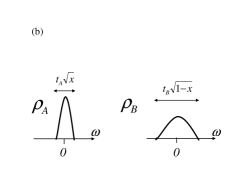
Choosing a Bethe tree structure as underlying lattice (this corresponds to a semi-elliptic DOS for the pure or pure system), we have computed and numerically for different values of the hopping elements. For the purpose of simplification, we present here some numerical results obtained for only. In the following, all energies are expressed in units of , where is the coordination number of the lattice, and different values of are considered.
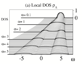
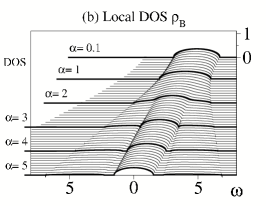
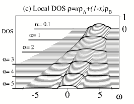
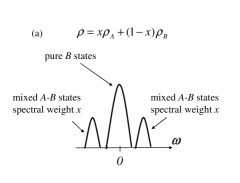
Figure 1 depicts the effect of off-diagonal randomness on the local DOS’s , , and . The plots presented here are obtained for a concentration of atoms of kind . Qualitatively similar behavior is found for different concentrations. For (), our numerical results recover the semi-elliptic DOS corresponding to a regular tight-binding model. In the regime , the DOS remains semi-elliptic like, with a rescaled bandwidth (see also FIG. 3 (b)). In the regime , the DOS corresponding to the minority atoms splits into two satellites peaks, centered around the energy , while the DOS corresponding to the majority atoms shows both a two satellites peak structure and a coherent peak around . The latter is reminiscent of the semi-elliptic one obtained in the absence of disorder (). As a consequence, the averaged local DOS is also characterized by a central peak and two satellites.
- Regime
Integrating the local DOS, we define the average densities
of electrons on sites and in the Fermi sea, as function of the
Fermi energy
| (116) |
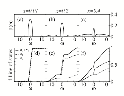
where and . We analyse in FIG. 2 the microscopical origin of the satellites and central peak in the averaged DOS for large values of . It appears that the two satellite peaks correspond to electronic excitations which are equally distributed over and sites, while the central peak is due to excitations of electrons on the majority sites. Our interpretation is the following: when , the electronic states with the lowest energy are obtained by forming bonds. The deepest levels of the Fermi sea thus correspond to electronic wave functions localized on clusters formed by alternating and atoms. In the following, we call the latter ” clusters”. We interprete the two satellite peaks as bonding and anti-bonding electronic states formed in these clusters. In the large limit, each atom can be associated with a neighboring atom . Choosing the latter to point into the same (arbitrary) ”direction” garantees that the so formed clusters contain exactely the same number of and atoms. As a consequence, the statistical weight of the clusters is , which is twice the concentration of the minority atoms . Whether a given site belongs to an cluster or to the embedding surface is left open. Nevertheless, the satellite peaks characterizing the DOS for have precisely the statistical weight , which is equaly distributed over and atoms (see FIG. 2 and FIG. 3 (a)). The remaining atoms constitute hypersurfaces embedding the clusters. Considering that the dimension of the system is proportional to , the embedding surfaces provide in the large limit a contribution to the DOS (central peak) which is qualitatively similar to the one obtained for (i.e., semi-elliptic here). The spectral weight of the latter is . Gaps in the local DOS, with two satellites and a central peak appear only above a critical value of . This is seen in FIG. 1.
- Regime
In the limit , the two subsystems and decouple, and the
averaged local DOS and can be deduced from the
DOS of a pure system by rescaling the
energy as and respectively
(see FIG. 3 (b)).
As a consequence, when , electrons with the lowest energy
occupy predominantly majority atoms.
When the density of conduction electrons is sufficiently large, the Fermi
level moves into a region where electrons occupy both and sites.
For that reason, the regime
is qualitatively not very different from the regime
, except in the limit of a low density of conduction
electrons.
V.2 Diagonal randomness: Kondo alloy
We consider next the transition between a diluted and a dense Kondo system. The model is defined by the KAM Eq. (1), with a periodic hopping element for the conduction electrons . The limit corresponds to a single impurity Kondo model (SIKM), while describes a Kondo lattice model (KLM). These models have been extensively studied [KondoHewson, ] by using various approximations. When we consider a paramagnetic ground state, two energy scales are required [Anderson2scales1, -Anderson2scales2, -Anderson2scales4, ] in order to describe the low temperature physical properties: characterizes the onset of the Kondo effect, and characterizes the formation of a coherent Fermi liquid ground state.
On one side, the exact solution of the SIKM, based on the Bethe Ansatz [NAndrei1, -NAndrei4, ] proves that these two scales are identical in the dilute limit . The low temperature physical properties of the SIKM are thus universal (i.e., independent from the lattice structure, electronic filling and Kondo coupling) as soon as all the energy scales are rescaled by .
On the other side, for the KLM these two energy scales are different. In earlier works it had been suggested that for small conduction electron densities is strongly reduced, i.e., to because of conduction electron ”exhaustion” when singlet states form [exhaustionearly1, -exhaustionearly2, -Nozieresnoexhaustion, ]. However this has turned out not to be the case and [Nozieresnoexhaustion, -KondolatticelargeN, ].
The KAM which is studied here allows for describing the crossover between the dilute regime (with ) and the dense regime (with depending on the electronic filling). From the static local magnetic susceptibility at zero temperature , we define an energy scale , which provides a reasonable estimate of [KondolatticelargeN, ].
FIG. (4) depicts the evolution of the ratio for different values of the electronic filling . It starts from in the dilute limit , as expected for the SIKM. With decreasing filling this ratio is lower in the dense limit corresponding to the KLM. This shows clearly that the crossover between the dense and the dilute regimes occurs when the concentration of Kondo impurities is equal to the electronic filling . Note that similar results have been obtained recently by Kaul and Vojta for a sites square lattice (compare FIG. (4) with FIG. (2) of Ref. [Vojta, ]).
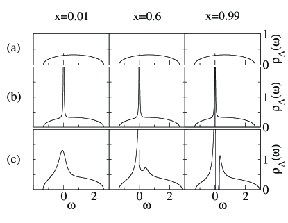
The above feature can also be observed from the spectral function , i.e., the local electronic DOS of a Kondo impurity. This is illustrated in FIG. (5) for an electronic filling of . Above the Kondo temperature, has the same semi-elliptic shape as in the absence of a localized spin. When a Kondo resonance develops at the Fermi level. Neither the quantitative value of nor the shape of the resonance depend on the concentration . This suggests that the onset of the Kondo effect at is not a collective coherent effect, but results from incoherent scattering of conduction electrons by the magnetic impurities. When the temperature is decreased far below the Kondo temperature, a collective coherent screening takes place, which is accompanied by the onset of the Fermi liquid regime. For the local DOS of sites depends on the concentration and shows in the dilute regime the standard Kondo resonance, while a gap occurs in the dense regime . We are aware that the presence of a Kondo gap is an artefact of the mean-field approximation which we have introduced. Numerical studies of the KLM without this approximation show however, that a pseudo-gap will form [KondolatticeCosti, ]. Similarly to what we obtained for the ratio , we find that the crossover between the dilute regime (without gap), and the dense regime (with a gap) occurs for . FIG. (5) depicts this behavior for an electronic filling . Similar results are obtained for .
Even without the exhaustion argument, it appears that the crossover between a dilute and a dense Kondo system occurs when the concentration of Kondo impurities is equal to the electronic filling . We expect this result to apply also to the Anderson model, which still contains the charge degrees of freedom associated with the spins of the sites. This explains why the single impurity models, characterized by a unique low temperature scale are still able to describe the low temperature properties of alloys with a significant concentration of magnetic impurities, here sites. As a consequence, in the experimental literature, the Kondo temperature of Kondo-like alloys is frequently estimated from different physical quantities, with no distinction beeing made between the quantities characterizing the Fermi liquid regime and those characterizing the onset of the Kondo effect. Nevertheless, two different energy scales, and , have been measured experimentaly and analysed for several rare earth alloys. For example, some very promising experimental results dedicated to an analysis of the crossover between diluted and dense impurity systems can be found in Ref. [ExperimentsYbLuAl, ] (alloy ), in Ref. [ExperimentsCeLaIrGe, ] (), or in Ref. [ExperimentsCeNiSi, ] ().
V.3 Combined effects of randomness
In this section we consider the KAM Eq. (1) with randomness of the electronic hopping matrix elements and of Kondo alloying effects. We study the effect of alloying, described respectively by the parameters and , and of randomness, characterized by the parameter defined by Eq. (115). For the sake of clarity we discuss here only the behavior of the two low temperature energy scales introduced in the previous section: the Kondo temperature , characterizing the onset of incoherent singlet formation, and , characterizing the onset of a coherent Fermi-liquid state. A good estimate of the latter can be obtained from the static local magnetic susceptibility at by the relation .
V.3.1 Kondo temperature
Next we study the effect of the concentration on the Kondo temperature by considering various values of randomness and electronic filling . The main variations we observe for result from the effects of randomness on the non interacting local DOS , which are analysed in Section V.1.
Figure 6 shows the dependence of the Kondo temperature with respect to . Without randomness (i.e., for ), the Kondo temperature does not depend on (see FIG. 6(b)). This reflects the fact that characterizes incoherent scattering of the conduction electrons on the spins . Due to the exponential dependence of on (see Eq. (47)), with possible gap opening (in the regime ) or bandwidth renormalisation (in the regime ), can be strongly reduced in certain regimes of concentrations as soon as .
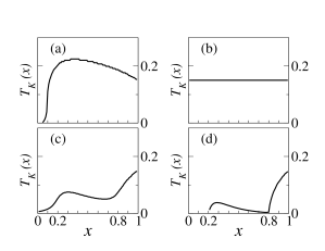
- Regime
A decrease of does not really change the value of , except
in the dilute regime , where is strongly reduced
(see FIG. 6(a)).
The reason is that when and are small, the effective bandwidth of the
local electronic DOS on sites is strongly reduced
(see FIG. 3 (b)).
Therefore the conduction electrons will fill the states at the non-magnetic
sites and is reduced.
- Regime
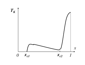
When increases, two critical concentrations and
occur. They define three regimes (see FIG. 6 (c) and (d),
and FIG. 7).
This is a consequence of the complex structure of the local DOS discussed
in Section V.1,
with a central and two satellite
peaks (see FIG. 3 (a)).
For , the Kondo or sites are in the majority. The Fermi level
is in the central peak of the DOS,
which precisely corresponds to electronic excitations on sites.
When decreases from to , the DOS is modified such that the
Fermi level approaches the band edge of the central peak.
As a consequence, decreases and can even vanish for if
is large enough.
For , the Fermi level is positioned in a satellite peak, corresponding to electronic excitations on both magnetic and non-magnetic sites. is finite but reduced compared to its value at . For , the Fermi level is in the central peak, but the latter corresponds now to excitations on the non-magnetic sites which here are in the majority. As a consequence, and are strongly reduced in this regime and can even vanish if is large enough.
Relations between , and the electronic filling can be obtained from the observation that the spectral weight of the satellite peaks is proportional to the concentration of the minority or sites. We thus find
| (117) | |||||
| (118) |
These relations corresponds to the critical values and obtained numerically for (see FIGS. 6 (c) and (d)). They are also verified by numerical results for other electronic fillings.
V.3.2 Kondo versus Fermi liquid temperature
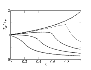
In the following we discuss the ratio between and . The effect of varying the electronic filling was discussed in Section V.2 for . Figure 8(b) reproduces for convenience the plot of as a function of corresponding to and shown in FIG. 4. The other plots of FIG. 8 depict the effect of varying with the electronic filling kept fixed. We obtained similar results with other values of . For the sake of clarity, we show here only the numerical results which we obtained for .
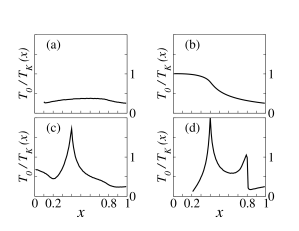
- Regime
The cross-over separating the dense and dilute regime is well
localized at and , and smoothed when decreases
(compeare FIG. 8 (a) and (b)).
At low concentrations, numerical calculations are less accurate.
This is related to the strong decrease of when
(see FIG. 6 (a)). For this reason, we are not able to
provide reasonable results concerning for .
- Regime
When increases, two different effects occur: the crossover between the
dense and dilute regime becomes more pronounced around
(see FIGS. 8 (c) and (d)) and some
”anomalies” occur at the critical concentrations
and (see Eqs. (118)).
When is approaching any of these critical values,
the ratio becomes small (see and
on FIG. 8 (d)).
Similar results were obtained for other values of
().
The general shape of the curve in the regime is
depicted by FIG. 9.
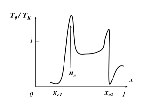
When , the physical properties of the system are
characterized by two universal temperature regimes:
for , the thermodynamic and transport properties are those of a
light Fermi liquid (due to the conduction electrons), and the magnetic
properties are characteristical of free moments (for example, the
magnetic susceptibility follows a Curie law).
For , the physical properties correspond to an heavy Fermi
liquid.
When , an intermediate regime occurs, corresponding
to , for which the temperature dependence of the
physical properties might have non-Fermi-liquid or spin-liquid behavior.
Note that the peak at in FIG. 8 (d) (and more generaly at on FIG. 9) has been explained in Ref [Kondopseudogap, ] to which we refer.
VI Summary and Conclusions
The aim of this investigation has been to develop a description of Kondo alloys, i.e., of systems with randomly placed Kondo ions of concentration . The values of were ranging from close to (diluted Kondo impurities) to (Kondo lattice). Different hopping matrix elements were assumed depending on wether the initial and final sites were Kondo sites or nonmagnetic sites. By expressing the spin of a Kondo site in terms of fermionic operators and by making a mean-field approximation we derived a Hamiltonian which has in addition to the conduction band a narrow band describing the low energy excitations of the system. The disorder of the system was treated by a (dynamical) coherent potential approximation (CPA) and by a dynamical mean-field theory (DMFT) approach. It was reconfirmed for the special system considered here that both approaches yield identical equations. For a practical application of the formalism a Bethe tree structure was chosen for convenience. It corresponds to working with a semi-elliptic density of states. Various quantities were calculated as function of the ratio , i.e., of different degrees of off-diagonal disorder and of Kondo ion concentration . Among them were the local density of states for the Kondo sites ( atoms) and for the nonmagnetic sites ( atoms). The averaged local densities of states depend strongly on the degree of disorder and on concentration . Of special interest was the case of diagonal randomness only. In that case and . The ratio between the Fermi liquid temperature and the Kondo temperature was investigated as function of , i.e., ranging from the impurity to the Kondo lattice limit. This ratio was shown to be of relevance for a number of experiments. Finally, a detailed study was presented for the case of a combined diagonal and off-diagonal disorder. In particular the behavior of the Kondo temperature as function of was studied in detail. The same holds true for the ratio of Fermi liquid to Kondo temperature. The latter can have a strong monotonic behavior as function of with peaks at different values of . They depend on the particular filling of the conduction band as well as on the parameter . Depending on the ratio we have obtained universal temperature regimes where the system has either properties of a liquid with light fermions and quasi-free local moments or of a liquid with heavy quasiparticles. There is also a temperature regime possible with non-Fermi liquid behavior. A still open question is under which conditions Luttinger’s theorem is inapplicable and how one can calculate in that case the volume enclosed by the Fermi surface. As is well known that volume does not include the electrons which form localized moments when we are in the regime of a light Fermi liquid. But they must be included when we are in the regime of heavy quasiparticles. Although the present investigation sheds some new light on Kondo alloys and their prperties there are important issues remaining for the future.
Acknowledgements.
We would like to thank N.B. Perkins for stimulating discussions during the early phase of this work. We thank M. Vojta for comments which helped us to improve the manuscript. We thank M. Capone, K. Kikoin, M. Laad and C. Lacroix for fruitful discussions.Appendix A CPA equations
A.1 Starting definitions
Considering the mean-field Kondo Alloy Model defined by the effective Hamiltonian Eq. (7), we define the Green’s function, transfer integral, and local propagator matrices, as
| (125) | |||||
| (133) |
The projection operator is unity if refers to site , and zero otherwise.
A.2 Equation of motion
The equations of motion derived from the Hamiltonian Eq. (7) for the scalar Green’s functions , , and , can be cast into the following matrix form:
| (134) |
We assume that the Green’s function and local propagator matrices can be inverted. This hypothesis can be satisfied by introducing a non zero parameter such that (or ) if is a site (respectively a site ). The limit is taken at the end of the calculations. Eq. (134) can then be expressed as
| (135) |
A.3 Local self-energy approximation
Generalising the CPA procedure of Ref. [matrixCPABEB1, -matrixCPABEB2, ], we assume that the averaged Green’s function matrix is characterised by a local self-energy matrix ,
| (136) |
where is the identity matrix. Averaging over a random distribution of sites and restores the translation symmetry of the underlying lattice. The averaged matrix Green’s function is periodic in space, and its Fourier transform is
| (137) |
Equation (135) can then be expressed as:
| (138) |
Next we establish a complete set of self-consistent equations for the Green’s function and the self-energy, whose matrix-elements are parametrised as follow
| (147) |
A.4 Off-diagonal blocks of : no double occupancy
A first set of relations is obtained by expressing the local averaged Green’s function in terms of their dependent conterparts.
| (151) |
Here is of the form of Eq. (138). Even if our approach artificially introduces two conducting bands and , the vanishing of the off-diagonal mixed matrix elements in prevents a double association of and atoms to the same site. The two corresponding equations determine the self-energy off-diagonal blocks and .
A.5 Diagonal blocks of : scattering of the effective medium
Self-consistent relations for and are obtained by requiring that the scattering of electrons of the effective medium by a given site vanishes on average. For a given random configuration of the alloy, and using Eqs. (135, 136), the Green’s function , is related to its average by
| (152) |
where
| (157) | |||||
The single-site scattering matrix on site is given by
| (158) | |||||
| (159) |
As mentioned above, the required matrix-inversions can be performed by introducing a non-zero parameter such that is equal to (site ) or (site ). We now consider the limit and we express the scattering matrix and on a site (respectively ). We find
| (165) |
and
| (171) |
with
| (174) | |||||
| (177) | |||||
| (178) |
We obtain the CPA equations for and by setting . The result is
| (181) | |||||
References
- (1) P. Fulde, P. Thalmeier, and G. Zwicknagl, Strongly correlated electrons, Solid State Physics 60 (Elsevier, 2006).
- (2) G. R. Stewart, Rev. Mod. Phys. 73, 797 (2001).
- (3) A.C. Hewson, The Kondo Problem to Heavy Fermions (Cambridge University Press, Cambridge, England, 1993).
- (4) J.R. Schrieffer, and P.A. Wolf, Phys. Rev. 149, 491 (1966).
- (5) V. Dobrosavljevic, T.R. Kirkpatrick, and G. Kotliar, Phys. Rev. Lett. 69, 1113 (1992).
- (6) E. Miranda and V. Dobrosavljevic, Phys. Rev. Lett. 78, 290 (1997).
- (7) S. Kettemann, and E.R. Mucciolo, JETP Letters 83, 240 (2006).
- (8) A.M. Sengupta, and A. Georges, Phys. Rev. B 52, 10295 (1995).
- (9) A.H. Castro Neto, G. Castilla, and B.A. Jones, Phys. Rev. Lett. 81, 3531 (1998).
- (10) S. Burdin, D.R. Grempel, and A. Georges, Phys. Rev. B 66, 045111 (2002).
- (11) R.K. Kaul, and M. Vojta. cond-mat/0603002.
- (12) J.A. Blackman, D.M. Esterling, and N.F. Berk, Phys. Rev. B 4, 2412 (1971).
- (13) D.M. Esterling, Phys. Rev. B 12, 1596 (1975).
- (14) A. George, G. Kotliar, W. Krauth, and M.J. Rozenberg, Rev. Mod. Phys. 68, 13 (1996).
- (15) W. Metzner and D. Vollhardt, Phys. Rev. Lett. 62, 324 (1989).
- (16) C. Lacroix and M. Cyrot, Phys. Rev. B 20, 1969 (1979).
- (17) B. Coqblin, M.A. Gusmao, J.R. Iglesias, C. Lacroix, A. Ruppenthal, A.S.D. Simoes, Physica (Amsterdam) 282B, 50 (2000).
- (18) N. Read, D.M. Newns, and S. Doniach, Phys. Rev. B 30, 3841 (1984).
- (19) D.M. Newns and N. Read, Adv. Phys. 36, 799 (1987).
- (20) P. Coleman, Phys. Rev. B 35, 5072 (1987).
- (21) See, for example, P. Fulde, Electron correlations in molecules and solids, 3rd enlarged ed. (Springer series in Solid State Sciences, Berlin, 1995).
- (22) P. Soven, Phys. Rev. 156, 809 (1967).
- (23) D.W. Taylor, Phys. Rev. 156, 1057 (1967).
- (24) B. Velicky, S. Kirkpatrick, and H. Ehrenreich, Phys. Rev. 175, 747 (1968).
- (25) H. Hasegawa, and J. Kanamori, J. Phys. Soc. Jpn. 31, 382 (1971).
- (26) S. Burdin, A. George, and D.R. Grempel, Phys. Rev. Lett. 85, 1048 (2000).
- (27) M. Jarrell, and H.R. Krishnamurthy, Phys. Rev. B 63, 125102 (2001).
- (28) Y. Kakehashi, Phys. Rev. B 66, 104428 (2002).
- (29) A. Chattopadhyay, S. Das Sarma, and A.J. Millis, Phys. Rev. Lett. 87, 227202 (2001).
- (30) M. Jarrell, H. Akhlaghpour, and T. Pruschke, Phys. Rev. Lett. 70, 1670 (1993).
- (31) A.N. Tahvildar-Zadeh, M. Jarrell, and J.K. Freericks, Phys. Rev. Lett. 80, 5168 (1998).
- (32) Th. Pruschke, R. Bulla, and M. Jarrell, Phys. Rev. B 61, 12799 (2000).
- (33) N. Andrei, Phys. Rev. Lett. 45, 379 (1979).
- (34) P. Wiegman, JETP Letter 31, 392 (1980).
- (35) P. Nozières, Ann. Phys. (Paris) 10, 19 (1985).
- (36) P. Nozières, Eur. Phys. B 6, 447 (1998).
- (37) P. Nozières, J. Phys. Soc. Jpn. 74, 4 (2005).
- (38) T. Costi, and N. Manini, J. Low Temp. Phys. 126, 835 (2002).
- (39) E.D. Bauer, C.H. Booth, J.M. Lawrence, M.F. Hundley, J.L. Sarrao, J.D. Thompson, P.S. Riseborough, T. Ebihara, Phys. Rev. B 69, 125102 (2004).
- (40) R. Mallik, E.V. Sampathkumaran, P.L. Paulose, J. Dumschat, and G. Wortmann, Phys. Rev. B 55, 3627 (1997).
- (41) E.D. Mun, Y.S. Kwon, and M.H. Jung, Phys. Rev. B 67, 033103 (2003).
- (42) S. Burdin, and V. Zlatic, cond-mat/0212222.