Particle redistribution and slow decay of correlations in hard-core fluids on a half-driven ladder

Abstract

We study driven particle systems with excluded volume interactions on a two-lane ladder with periodic boundaries, using Monte Carlo simulation, cluster mean-field theory, and numerical solution of the master equation. Particles in one lane are subject to a drive that forbids motion along one direction, while in the other lane the motion is unbiased; particles may jump between lanes. Despite the symmetry of the rates for transitions between lanes, the associated particle densities are unequal: at low densities there is an excess of particles in the undriven lane, while at higher densities the tendency is reversed. Similar results are found for an off-lattice model. We quantify the reduction in the stationary entropy caused by the drive. The stationary two-point correlation functions are found to decay algebraically, both on- and off-lattice. In the latter case the exponent governing the decay varies continuously with the density.

I Introduction

Over the last decades considerable effort has been devoted to the investigation of simple nonequilibrium models of interacting particles. In addition to their application to specific problems (traffic flow, ionic conductors, epidemics, etc.), such studies have been motivated by the hope of developing a macroscopic description of far-from-equilibrium systems. Driven lattice gases, also known as driven diffusive systems (DDS) zia ; schutz ; marro , have played an important role in this program. In these models, a stochastic lattice gas is subject to a “drive” that biases hopping along one of the principal axes of the lattice kat83 . The repulsive version leu89 ; dic90 ; szabo94 ; szabo96 serves as a model for fast ionic conductors boy79 . Stationary properties of driven lattice gases depend strongly on the details of dynamics, unlike in equilibrium. DDS have provided a wealth of unexpected and counterintuitive results, many of which remain to be fully explained zia . (For example: the fact that the critical temperature of the attractive lattice gas increases under driving.)

Recently, a study of a two-dimensional lattice gas with nearest-neighbor exclusion (NNE), subject to a nonuniform (shear-like) drive, revealed a tendency for particles to migrate to the region with weaker drive nne-shear ; the accumulation of particles is sufficiently strong to provoke sublattice ordering in this region. At higher densities the trend reverses, with particles accumulating in jammed regions that form where the drive is strongest. To better understand these results, we consider, in the present work, a one-dimensional (ladder) analog of the model studied in Ref. nne-shear . The reduced dimensionality permits us to obtain simulation results of high precision, to develop high-order cluster approximations, and to derive essentially exact results (for smaller systems), via numerical solution of the master equation. We find that particles migrate preferentially to the undriven lane at low densities, and to the driven one at higher densities. The same tendencies are observed in simulations of a continuous-space model.

In our model, one ring corresponds, in isolation, to a totally asymmetric exclusion process (TASEP) with sequential dynamics, while the other is a symmetric exclusion process. (Note however that the most widely studied version of the TASEP features on-site exclusion only.) Both models are exactly soluble and possess a stationary probability distribution that is uniform on the set of allowed configurations. The interaction between particles on different rings and the possibility of jumping between them changes this situation: the stationary probability distribution is no longer uniform, and the model exhibits nontrivial behavior. (The ladder without driving in either lane again corresponds to a simple equilibrium model that can be solved exactly via the transfer-matrix technique.) The TASEP has attracted much attention due to the phase transitions that arise when, instead of periodic boundaries, the end sites are coupled to particle reservoirs derrida98 ; schutz ; krug ; derrida ; kolomeisky . Although not directly to the system studied here, it is worth noting that quite surprising phase behavior is found in an interacting TASEP ladder, when the two lanes are coupled to different reservoirs popkov , or there are asymmetric transition rates between them pronina . A single-lane TASEP with repulsive nearest-neighbor interactions exhibits a surprisingly complex phase diagram popkov99 .

Our focus in this paper is on stationary properties, specifically, the particle density in the two lanes, the current, and the two-point correlation function. We also examine the stationary probability distribution (for the lattice model) on configuration space, and show that this distribution does not admit a simple characterization in terms of a set of macroscopic variables. The two-point correlation function $h(r)$ exhibits power-law decay in both the lattice and continuous-space models. Algebraic decay of correlations is well established in DDS zia ; zhang88 , and is expected to be a generic feature of anisotropic nonequilibrium systems with a conserved density garrido90 , but is not commonly observed in periodic, one-dimensional systems.

The balance of this paper is organized as follows. In the next section we define the models, and in Sec. III discuss the stationary solution of the master equation for the lattice gas model. Cluster approximations are developed in Sec. IV. In Sec. V we report simulation results, and in Sec. VI present a qualitative explanation of the migration observed at low density. We close in Sec. VII with a discussion of our findings.

II Model systems

We consider particle systems with excluded-volume interactions on ladders with periodic boundaries. The position of particle $i$ is $(x_{i},y_{i})$, where $y_{i}\in\{1,2\}$ denotes the lane. In the lattice gas model, $x_{i}\in\{1,2,...,L\}$; in the off-lattice model $x_{i}\in[0,L]$. In both cases, there are periodic boundaries in the $x$ direction. Interactions between particles are purely repulsive: in the lattice gas model, the minimum allowed distance between particles in the same lane is 2, while for particles in different lanes, the minimum allowed separation is 1. (Note that the NNE condition means there is no particle-hole syttetry.)

In the off-lattice model the minimum distance between particles in the same lane is 1, while the minimum separation along $x$, for particles in different lanes is $1/2$. The maximum density is 1 in this case. In both the lattice gas and continuous-space models, the excluded volume constraint makes it impossible for particles to pass one another: the order of particles along the $x$ direction cannot change.

The process evolves via a sequential (continuous-time) Markovian dynamics. In the lattice gas, each particle in the driven lane ($y=2$) attempts to hop forward by one lattice spacing [$(x,2)\to(x+1,2)$] at rate $\alpha$, and to hop to the other lane [$(x,2)\to(x,1)$] at rate $\beta$. Particles in the undriven lane ($y=1$) attempt to hop to the upper lane at rate $\beta$, and to hop forward or backward, each at rate $\gamma$. Any attempted move that does not violate the excluded-volume constraint is accepted. The continuous-space model follows a similar dynamics. The rate of interlane driven transitions is again $\beta$. In the driven lane, the intralane hopping rate is $\alpha$, with the displacement $\Delta x$ uniformly distributed on $[0,1]$, so that particles in this lane cannot jump in the $-x$ direction. The hopping rate within the undriven lane is $\gamma$; the displacement is uniformly distributed on $[-1/2,1/2]$. Fig. 1 shows a typical region in the continuous-space model.

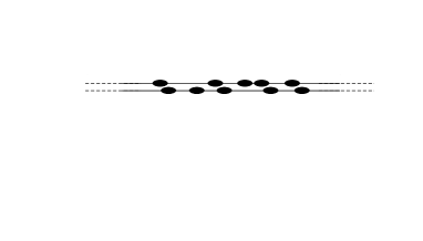
Figure 1: Typical region in the continuous-space model. Particles in the upper lane may only move to the right.

The parameters characterizing the system are its size $L$, particle number $N$, and the transition rates $\alpha$, $\beta$, and $\gamma$. We expect that for large $L$, macroscopic properties depend on the particle density $\rho=N/(2L)$ instead of on $N$ and $L$ separately. In general, stationary properties depend on the transition-rate ratios ($\tilde{\beta}\equiv\beta/\alpha$ and $\tilde{\gamma}\equiv\gamma/\alpha$, for example). The models (on- or off-lattice) with unbiased dynamics in both lanes represent equilibrium fluids with purely excluded volume interactions. In this case the stationary probability distribution is uniform on the set of allowed configurations. The NNE lattice gas with both lanes driven also possesses a uniform stationary distribution, provided any absorbing configurations (see below) are excluded from consideration. (To show this one verifies that the number of configurations accessible from a given configuration ${\cal C}$ equals the number of configurations from which ${\cal C}$ is accessible, and that each transition out of ${\cal C}$ occurs at the same rate as the corresponding transition in. It is easy to verify that this symmetry no longer holds in the half-driven ladder.) The same holds for the half-driven ladder with on-site exclusion only. We should therefore expect these models to have a trivial behavior (for example, exponentially decaying correlations).

III Master equation

It is straightforward to write the master equation for the lattice gas model defined in the previous section, the only practical limitation coming from the rapid growth in the number of configurations and transitions with increasing system size. In both this and the following section we employ a base-3 notation in which the configuration $c$ in each column (fixed $x$) is denoted by 0, 1 or 2, corresponding to both sites empty, lower site occupied, or upper site occupied, respectively. Then a configuration on a ring of $2\times L$ sites is denoted by ${\cal C}=\sum_{j=1}^{L}3^{j-1}c_{j}$. Allowed configurations are such that, if $c_{j}=1$ or 2, $c_{j-1}\neq c_{j}$ and $c_{j+1}\neq c_{j}$, for $j=1$,…,$L$, with periodic boundaries.

Our analysis of the master equation involves three steps. First, we enumerate all allowed configurations of $N$ particles on a ladder of $2L$ sites; configurations that differ merely by a rotation are treated as equivalent. Next, the set of all transitions and associated rates is generating by considering all possible particle movements in each configuration. Finally, the stationary probability distribution is generated via the fast iterative method described in intme . (For an alternative approach to constructing the stationary distribution see zia06 .)

At higher densities, some of the allowed configurations are absorbing; all particle motion is blocked. This is obviously the case for $N=L$, which is of no interest here. For even $L$, however, absorbing configurations with $N<L$ are possible; instances appear for $N$ as small as $2L/3$, if $L$ is a multiple of six. (In particular, all configurations with $N=L-1$ are absorbing for $L$ even.) It turns out that all absorbing configurations are isolated in the sense that there are no transitions into them from other configurations. We therefore eliminate such configurations from the state space. (In simulations the initial configuration is always chosen to be nonabsorbing.) We have verified, for systems of up to 38 sites, that the process (restricted, if necessary, to the nonabsorbing subspace) is ergodic, i.e., there is a sequence of transitions leading from a given configuration to any other.

The stationary probability distribution $\overline{p}_{i}$ is used to evaluate the particle and current densities in each lane, and the statistical entropy per site, $s=-\frac{1}{2L}\sum_{i}\overline{p}_{i}\ln\overline{p}_{i}$. We report results for the case $\alpha=2$, $\beta=\gamma=1$. Fig. 2 shows the fraction $R=\rho_{1}/\rho$ of particles in the nondriven lane ($y=1$) for several system sizes. For densities less than about 0.3, there is an excess of particles in the undriven lane; the excess appears for systems with three or more particles. For densities above 0.3, the trend reverses, with an excess of particles appearing in the driven lane. Away from the extremes of $\rho\simeq 0$ and $\rho\simeq 1/2$, the fraction $R(\rho)$ appears to trace out a smooth, roughly sinusoidal curve. (Note however that this curve is not symmetric about the line $\rho=1/4$, nor about the line $R=1/2$.) We verified that in the absence of driving, the stationary probability distribution is uniform on the set of allowed configurations.

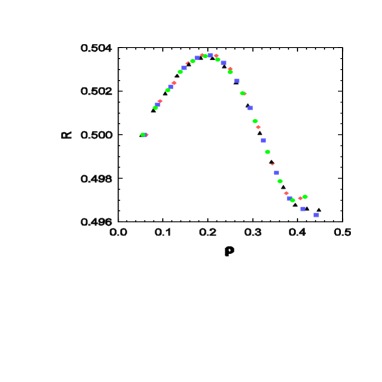
Figure 2: Stationary fraction $R$ of particles in the undriven lane versus total density $\rho$. Diamonds: $L=16$; squares: $L=17$; circles: $L=18$; triangles: $L=19$.

In Fig. 3 we show the current densities (mean rate of moves in the $+x$ direction, less the number in the $-x$ direction, divided by $L$), $j_{d}$ and $j_{u}$, in the driven and undriven lanes, respectively. As expected, the current in the driven lane first grows with $\rho$ (due to increasing number of carriers), and then decays (due to blocking of particle movement at higher densities); the maximum occurs at a density near 0.16. Due to the no-passing condition, particles in the undriven lane must also, on average, move forward. The current in this lane grows more slowly, reaching a maximum near $\rho\simeq 0.28$. At higher densities the currents in the two lanes are virtually identical, as movement in one implies a corresponding movement in the other.

The “outlying” points at high density in Fig. 3 reflect an odd-even effect that occurs near maximum filling. It is easy to verify, for example, that an isolated hole ($N=L-1$) is immobile for $L$ even, while for $L$ odd it has a stationary velocity of $2\alpha\gamma/(\alpha+2\gamma)$. Surprisingly, when $L$ is odd, the current for two holes is slightly less than for just one hole. These “anomalies” are also observed in simulations (Sec. V).

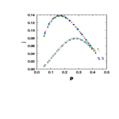
Figure 3: Stationary current density $j$ versus total density $\rho$. System sizes as in Fig. 2. Upper curve: driven lane; lower: undriven lane.

As noted, in equilibrium all allowed configurations have the same probability, so that the entropy (in units of Boltzmann’s constant) is $\ln\Omega(L,n)$, with $\Omega(L,n)$ denoting the number of configurations of $n$ particles on a ladder of $2L$ sites that satisfy the NNE condition. Under biased dynamics the stationary probability distribution is no longer uniform over the set of configurations, making the statistical entropy of the driven system smaller than in equilibrium. In Fig. 4 we plot the entropy difference per site, $\Delta s=s_{eq}-s$, versus $\rho$. The entropy reduction appears to attain a maximum near $\rho=0.22$. (For comparison we note that $R$ is maximum for $\rho\simeq 0.2$, while the current in the driven lane is maximum for $\rho\simeq 0.17$.) Under the nonequilibrium dynamics, curiously, configurations with a more or less even distribution between the lanes are favored. This is demonstrated in Fig. 5, which shows the average probability over all configurations with exactly $n$ particles in the driven lane, for the case $L=19$, $N=8$. (Of course, configurations with $n=N/2$ are more numerous, but in equilibrium the average probability is the same for all $n$.) The average probability is slightly higher for $n=3$ than for $n=5$, consistent with the migration of particles to the undriven lane. Note however that in the tails of the distribution ($n$=0, 1 compared with $n=$7, 8) this tendency is reversed.

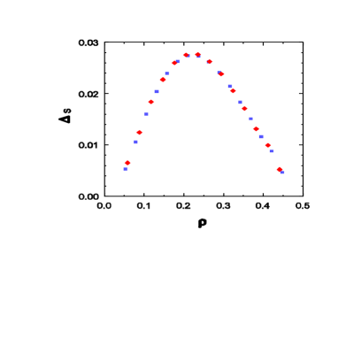
Figure 4: Entropy difference per site $\Delta s$ for $L=17$ (diamonds) and $L=19$ (squares).

Figure 5: Average stationary probability of configurations having exactly $n$ particles in the driven lane, $L=19$, $N=8$.

A related question is whether the stationary probability distribution $\overline{p}_{i}$ can be expressed in terms of a small set of variables. The ‘natural’ set of variables characterizing the global state of the system would appear to be the current densities $j_{d}$ and $j_{u}$ and the density $\rho_{d}$ of particles in the driven lane. Classifying configurations by the values of these three variables, however, we find large variations in $\overline{p}_{i}$ within each class. (In fact, for classes with more than one element, the standard deviation of $\overline{p}_{i}$ over the class is comparable to the mean stationary probability of the class.) For example, in the case $L=16$, $n=8$, the most numerous class, with 1497 configurations, is that having $n_{d}=4$, and total currents $J_{d}=4$ and $J_{u}=0$. Within this class the stationary probabilities vary over two orders of magnitude (from $1.3\times 10^{-6}$ to $1.23\times 10^{-4}$), and almost all are distinct. (There is just one pair of configurations that have the same probability.) We therefore conclude that unlike in equilibrium, the stationary probability distribution cannot be written as a function of a reduced set of variables.

IV Cluster approximations

Numerical solution of the master equation, discussed in the previous section, furnishes essentially exact results for limited system sizes. In this section we apply a complementary approach that treats effectively infinite systems using dynamic cluster approximations marro ; mancam . We work with clusters of $2n$ sites (“$n$-column approximation”). For a given cluster size, we enumerate all configurations and all possible transitions involving the movement of a particle into, out of, or within the cluster. Next we consider the master equation for the probability distribution on this set of configurations. For certain transitions, the contributions to the gain and loss terms in the master equation can be written exactly using the $n$-column probability distribution. In other cases, however, the probability of a larger configuration, involving $n+1$ or $n+2$ columns, is needed to evaluate the contribution. Such probabilities are approximated in terms of the $n$-column probabilities.

Figure 6: Examples of transitions considered in the cluster approximation.

Consider, for example, the transitions depicted in Fig. 6. Using the notation defined in the previous section, the starting configurations are denoted 6, 21, and 11, in cases a, b, and c, respectively. We denote the probability of configuration $i$ on a set of $n$ columns as $p_{n}(i)$. In case a, the contribution to the loss term in $dp_{3}(6)/dt$ [and to the corresponding gain term for $p_{3}(3)$] is simply $\beta p_{3}(6)$, since this transition does not depend on the state of any sites outside the 3-column cluster. In case b, the transition is only possible if the site immediately to the right of the target site is vacant. This transition therefore involves the 4-column probabilities $p_{4}(63)$ and $p_{4}(65)$. Using the factorization $p_{4}(63)\simeq p_{3}(21)p_{3}(9)/p_{2}(3)$ and the analogous expression for $p_{4}(65)$, the contribution (to the loss term for $p_{3}(21)$, in this case) due to this transition is

$$R_{b}=\gamma\frac{p_{3}(21)[p_{3}(9)+p_{3}(11)]}{p_{2}(3)}.$$ (1)

Similar reasoning leads, in case c, to the expression

$$R_{c}=\alpha\frac{p_{3}(11)p_{3}(6)[p_{3}(18)+p_{3}(19)]}{p_{2}(2)p_{2}(6)}.$$ (2)

In general, in the $n$-column approximation, an ($n\!+\!1$)-column probability is given by the product of the corresponding $n$-column probabilities divided by the ($n\!-\!1$)-column probability corresponding to the overlap region. (The latter is a marginal probability obtained from the $n$-column probability distribution.) Probabilities of ($n\!+\!2$)-column clusters are similarly estimated as the product of three $n$-column probabilities divided by the product of two ($n\!-\!1$)-column probabilities.

The systems of equations for 1, 2 and 3 columns are readily constructed by hand, but to study larger clusters we develop a computational algorithm that generates all possible transitions on an $n$-column cluster, and applies the approximation scheme defined above systematically. The same routine integrates the resulting set of coupled ODEs numerically using the fourth-order Runge-Kutta scheme. Due to relatively slow convergence, we limited this study to $n\leq 7$ columns. The predictions of the cluster approximation are compared against simulation in the following section.

To close this section we comment on a subtlety arising in the definition of the initial probability distribution. Valid $n$-column distributions must satisfy certain symmetry relations, due to the fact that, in general, the marginal distributions for $m<n$ columns can be written in several ways. Consider the case $n=2$, for which the possible configurations are 0, 1, 2, 3, 5, 6, and 7. In addition to normalization, the following constraints apply to the two-column probability distribution:

$$p_{2}(3)+p_{2}(5)=p_{2}(1)+p_{2}(7)=p_{1}(1)=\rho_{1}$$ (3)

and

$$p_{2}(6)+p_{2}(7)=p_{2}(2)+p_{2}(5)=p_{1}(2)=\rho_{2}$$ (4)

For $n=3$ further constraints arise, for example:

$$p_{3}(2)+p_{3}(20)+p_{3}(11)=p_{3}(6)+p_{3}(7)=p_{2}(2)$$ (5)

and

$$p_{3}(15)+p_{3}(16)=p_{3}(5)+p_{3}(23)=p_{2}(5)$$ (6)

Since the total density $\rho$ is conserved by the equations of motion, it must be defined in the initial distribution: $\rho=(1/2L)\sum_{j}N_{j}p_{n}(j,t=0)$, where $N_{j}$ denotes the number of occupied sites in configuration $j$. For small clusters it is possible to find a simple parametrization of the probability distribution that permits one to fix the density while satisfying the symmetry relations noted above. But for large $n$ this becomes increasingly more complicated. To circumvent this difficulty, we generate the initial distribution for the ladder by integrating the equations of motion for the probability distribution (in the $n$-column approximation), for a different process, namely, the equilibrium lattice gas with nearest-neighbor exclusion, evolving via single-particle adsorption and desorption. In this process the fugacity $z$ controls the equilibrium density. We start with density zero; at any subsequent moment the probability distribution satisfies the conditions noted above, since they are intrinsic symmetries of the equations of motion. (In practice we halt the integration when the density $\rho$ has reached the value we wish to study in the driven model. There is no need to run the adsorption-desorption model to equilibrium.)

V Simulation results

V.1 Lattice gas model

We perform Monte Carlo simulations of the lattice gas model defined in Sec. II on ladders of $2\times L$ sites with periodic boundaries, using $L=200$ and 1000. The results reported here represent an average over 4 to 10 independent realizations. In each case, we verified that the system had reached the steady state. In Fig. 7 we show the density ratio $R=\rho_{1}/\rho$ for transition rates $\alpha=2/3$, $\beta=\gamma=1/3$; its behavior is very similar to that observed in the stationary solution of the master equation, Fig. 2. Excellent agreement between simulation and the cluster approximation (shown here for $n=7$) is also evident. Similar observations apply to the currents, depicted in Fig. 8. [It is worth noting that small cluster approximations do not provide good predictions. For example, it is only for $n\geq 4$ that the approximation predicts the migration to the driven lane ($R<1/2$), observed at higher densities.] Studies using $L=1000$ reveal little difference from the results for $L=200$ shown in Figs. 7 and 8, so that finite-size effects appear to be quite weak in this system. In fact, $R$ is only slightly less than found in the studies of much smaller systems (Fig. 2). The current densities are also comparable if one recalls that the rates used in the simulations are 1/3 those used in the master equation studies. The odd-even effects noted in the latter analysis reappear here, as shown in the inset of Fig. 8, where the total current in each lane is plotted versus the number of holes, $n_{h}\equiv L-N$. The currents are quite different for $n_{h}\leq 4$.

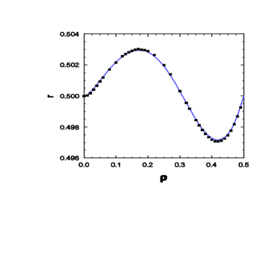
Figure 7: Stationary fraction $R$ of particles in the undriven lane versus total density $\rho$, in simulations with $L=200$ (points) compared with the seven-column cluster approximation (curve).

Figure 8: Stationary current densities $j_{d}$ (upper set) and $j_{u}$ (lower set) versus total density $\rho$, in simulations with $L=200$ (points) and the seven-column cluster approximation (curve). Inset: total current versus number of holes, for $L=50$ (squares: undriven lane, $\times$: driven) and $L=51$ (triangles: undriven, $+$: driven); dashed lines are to guide the eye.

Varying the hopping rates, the magnitude of the density shift changes. Fixing $\rho=0.17$, the value for which $R$ is maximum in Fig. 7, we obtain the largest value, $R=0.5065$, for $\beta/\alpha\geq 10$ and $\alpha/\gamma\geq 10$. In the opposite limit, $\gamma/\alpha\geq 10$, we observe very little migration ($|R-1/2|\simeq 10^{-4}$), regardless of the value of the interlane transition rate $\beta$. The density imbalance also disappears when we remove excluded-volume interactions between particles in different lanes.

Some insight into the dynamics is afforded by a space-time plot of the evolution. Fig. 9 shows the configuration at unit time intervals, in a system that has already relaxed to the stationary state. (Time increases downward in the figure. Particles in different lanes are given different colors.) There are rarefied, high-mobility regions separated by “bottlenecks” that typically form behind a diagonal pair of particles, with the one to the right in the undriven lane.

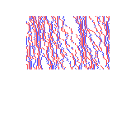
Figure 9: Space-time evolution, as explained in text. Rates $\alpha=2/3$, $\beta=\gamma=1/3$, density $\rho=0.17$.

Correlations in the driven system are quite different from those in equilibrium. In this model we may distinguish four radial distribution functions (RDFs): $g_{uu}$, $g_{dd}$, $g_{ud}$ and $g_{du}$. In each case, $g_{mn}(r)$ is proportional to the probability of sites $i$ and $i+r$ (in lanes $m$ and $n$, resp.), being occupied simultaneously, and is normalized so that $g_{mn}(r)\to 1$ for $r\to\infty$. In Fig. 10 we compare the RDFs with the corresponding equilibrium distributions, for density $\rho=0.125$. (In equilibrium we need only distinguish $g_{s}$, for sites in the same lane, and $g_{d}$, for sites in different lanes.) Correlations are generally stronger in the driven system than in equilibrium, especially for $g_{du}$ at contact, reflecting the accumulation of driven particles just behind undriven ones. It is also evident that $g_{uu}$ decays more slowly than the corresponding equilibrium RDF.

The slow decay is in fact shared by all of the RDFs in the driven system; each appears to follow a power law. In Fig. 11 we plot the correlation function $h(r)=g(r)-1$ on log scales, where $g(r)$ denotes the average of the four RDFs defined above. The correlation function follows $h(r)\propto r^{-\phi}$ with $\phi=2.11(3)$ for density $\rho=0.125$. We observe similar power-law tails in $h(r)$ at other densities (up to $\rho=0.3$), with decay exponents $\phi\approx 2$, as summarized in Table I. (These results were obtained using systems with $L\geq 500$ sites.) At higher densities the RDF exhibits damped oscillations with an exponentially decaying amplitude: $|h(r)|\propto e^{-r/\xi}$, as in equilibrium. (For $\rho=0.4$, for example, we find $\xi\simeq 3.4$.) In fact, the RDFs at high density differ from their equilibrium counterparts by only a few percent. The power-law tail may still be present at high density, but due to its low amplitude it tends to be masked by the oscillations (for smaller $r$) and noise (at larger $r$).

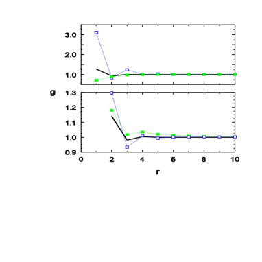
Figure 10: Radial distribution functions, density $\rho=0.125$, $L=200$. Lower panel: filled symbols: $g_{uu}$: open symbols: $g_{dd}$, solid line: $g_{s}$ (equilibrium). Upper panel: filled symbols: $g_{ud}$: open symbols: $g_{du}$, solid line: $g_{d}$ (equilibrium).

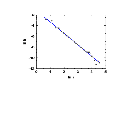
Figure 11: Correlation function $h(r)$ for density $\rho=0.125$. The slope of the line is -2.11.

$\rho$	$\phi$
0.05	1.93(4)
0.1	1.98(2)
0.125	2.10(3)
0.15	1.96(2)
0.20	1.99(3)
0.25	1.95(5)
0.30	2.16(13)

Table I. Values of the exponent $\phi$ governing the decay of the two-point correlation function in the lattice model with $\alpha=2/3$ and $\beta=\gamma=1/3$.

As the particle density tends to its maximum value of 1/2, the density of mobile vacancies $\rho_{m}$ approaches zero linearly [$\propto(1/2-\rho)$], as does that of mobile particles. For a vacancy to be mobile, it must be capable of exchanging places with a neighboring particle, which means that the vacancy must have exactly one occupied nearest neighbor. In the undriven lane, this can be any of the three neighboring sites, but for a vacancy in the driven lane, the neighboring particle must be below or to the left, for it to be mobile. Thus at low density we expect the density $\rho_{m,d}$ of mobile vacancies in the driven lane to be 2/3 that in the undriven lane, as is verified in simulations. Surprisingly, at high density the disparity becomes much greater, the ratio $\rho_{m,d}/\rho_{m,u}$ tending to 1/4 as $\rho\to 1/2$. At the same time, there is a marked tendency for mobile vacancies to cluster in the driven layer; the contact value of the associated RDF is $\simeq 8$ at density 0.49.

V.2 Continuous-space model

We also performed simulations of a system in which, as described in Sec. II, the $x$-coordinate of a particle can vary continuously on the interval $[0,L]$, again with periodic boundaries. A preliminary investigation showed that migration to the undriven lane is strongest (for densities near 0.17) for rates $\alpha=0.8$, $\beta=1$, and $\gamma=0.1$. Using these values, we study the dependence of the lane densities and currents as a function of overall density $\rho$, in systems of size $L=200$ and 1000. The fraction $R$ of particles in the undriven lane (Fig. 12) shows the same general tendencies as in the lattice gas, but the initial rise with density $\rho$ is more rapid, and the reverse migration at high densities is weaker than on the lattice. The current densities (Fig. 13) are again qualitatively similar to those found in the lattice model.

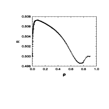
Figure 12: Stationary fraction $R$ of particles in the undriven lane versus total density $\rho$, in simulations of the continuous-space model with rates $\alpha=0.8$, $\beta=1$, and $\gamma=0.1$. Open squares: $L=200$; filled squares: $L=1000$.

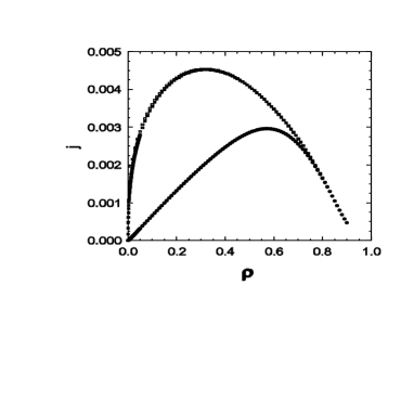
Figure 13: Stationary current densities $j_{d}$ (upper set) and $j_{u}$ (lower set) versus total density $\rho$, in in simulations of the continuous-space model, parameters as in Fig. 12.

Examples of RDFs in the continuous-space model are plotted in Figs. 14 and 15 for density $\rho=0.1$; they exhibit the familiar peak near contact and damped oscillations. The value at contact however is much larger than in equilibrium, where for the Tonks gas $g(1)=1/(1-\rho)$. In particular, $g_{du}$ (Fig. 15) becomes extremely large as $r\to 0.5$, reflecting the pile-up of driven particles behind undriven ones in the opposite lane. This feature allows to understand why the RDF in the undriven lane attains its maximum near $r=1.5$ rather than $r=1$. Given the exceptionally large value of $g_{du}$ near $r=0.5$, we expect (and in fact observe) a secondary maximum in this function near $r=1.5$, due to situations in which particles $i-1$ and $i$ are in the driven lane and $i+1$ is in the undriven one. The maximum in $g_{uu}$ near $r=1.5$ is due to events in which particle $i-1$ jumps to the undriven lane.

To obtain precise results for the correlation functions $h_{\alpha\beta}=g_{\alpha\beta}-1$ at large $r$ we performed studies using larger systems (5000 - 20 000 sites) and improved statistics (6 - 10 independent runs consisting of $\geq 2\times 10^{8}$ time steps). (Since all four correlation functions show the same behavior for large $r$, we study the mean of the four, denoted simply as $h(r)$.) At the lowest densities studied ($\rho=0.01$ and 0.02, using $L=20\,000$) we find a clear power-law decay over more than two decades (see Fig. 16). Comparing Figs. 16 and 11, one sees that in continuous space, the amplitude of the power law is nearly two orders of magnitude larger than on the lattice. For $\rho\geq 0.03$, the correlation function $h(r)$ decays in a nonmonotonic fashion: it is negative for $r>r^{*}$, and approaches zero from below as $r\to\infty$ (see Fig. 16 inset). In these cases we cannot fit $h(r)$ with a simple power law, but have obtained excellent fits (for $r<r^{*}$), introducing one further adjustable parameter, in the functional form

$$H(r)\simeq Ar^{-\phi}\left(1-\frac{r}{r^{*}}\right)^{\psi}$$ (7)

(Note that $r^{*}$ is determined from the simulation data and is not an adjustable parameter. $\phi$ and $\psi$ are obtained by minimizing the variance of $\ln h(r)-\ln H(r)$, ignoring the additive constant $A$. The latter is obtained once the two exponents have been determined.) The simulation data and associated fits are shown in Fig. 16; the parameters, listed in Table II, suggest that the decay exponent $\phi$ varies systematically with density. (We cannot fit the region of negative $h(r)$ using this function; the data for $\rho=0.05$ shown in the inset of Fig. 16, suggest that $|h(r)|\sim 1/r$ in this regime.)

Preliminary results indicate that $\phi$ also depends on the transition rates. Fixing the density at $\rho=0.05$, the rates $\alpha=0.8$, $\beta=1$, and system size $L=1000$, we find $\phi=1.21(7)$, 1.15(2), and 1.51(2) for $\gamma=0.02$, 0.1, and 0.5, respectively. For density $\rho=0.25$ the correlation functions have an oscillatory structure; the initial decay is exponential, with an associated correlation length of about 3.2. We verify that when both lanes are driven, the correlation function decays exponentially, as expected.

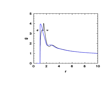
Figure 14: Stationary radial distribution function $g(r)$ in the continuous space model, $\rho=0.1$, $L=200$, for particles in the same lane; d: driven lane; u: undriven lane.

Figure 15: Stationary radial distribution function $g(r)$ as in Fig. 14, for particles in different lanes; upper panel: $g_{du}$; lower: $g_{ud}$.

$\rho$	$\phi$	$\psi$	$r^{*}$
0.01	0.87(1)	-	-
0.02	1.02(1)	-	-
0.03	1.10(3)	1.47(3)	317.3
0.04	1.14(2)	1.37(3)	212.7
0.05	1.19(3)	1.44(3)	173.3
0.1	1.28(3)	1.43(3)	68.7
0.15	1.49(4)	1.36(4)	45.5

Table II. Exponent $\phi$ and related parameters characterizing the two-point correlation function in the continuous-space model. Transition rates $\alpha=0.8$, $\beta=1$, and $\gamma=0.1$, system size $L\geq 5000$.

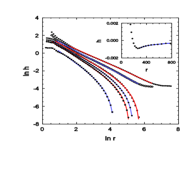
Figure 16: Correlation function $h(r)$ for (upper to lower) $\rho=0.01$, 0.02, 0.03, 0.04, 0.05, and 0.10. Lines represent fitting functions: a simple power law for $\rho\leq 0.02$, and the function $H(r)$ defined in Eq. 7 for $\rho\geq 0.03$. Inset: detail of $h(r)$ for large $r$ on linear scales; fitting function: -$0.25/r$.

VI Redistribution mechanism

The cluster approximation developed in Sec. IV reproduces the simulation results to high accuracy, but does not explain the observed migration of particles. In this section we suggest a mechanism for this phenomenon, based on the tendency (as revealed in the correlation functions discussed above) for diagonal pairs of particles to form, with the particle to the left in the driven lane [that is, pairs of the form $(x,2)$, $(x\!+\!1,1)$]. Given that such pairs are relatively long-lived, it is interesting analyze the problem of a third particle in the presence of such a pair.

Suppose the fixed pair occupies sites (0,2) and (1,1) on a ring of $2L$ sites. Then the third particle is free to visit sites $(3,1),(4,1),...,(L\!-\!1,1)$ and $(2,2),(3,2),...,(L\!-\!2,2)$. In the stationary state the third particle will tend to be found close to, and to the left of, the fixed pair, and the stationary probability $\overline{p}(L\!-\!j,y)$ should decay exponentially with $j$ due to the rightward drift. It turns out that in this situation, the third particle has a higher probability to be found in the undriven lane than in the driven one, as we now show.

From here on we refer to the third particle simply as the ‘particle’, and analyze the master equation describing this biased random walk, which is subject to reflecting boundaries, due to the fixed pair. Denoting by $p(x,y,t)$ the probability for the particle to be at site $(x,y)$ at time $t$, we have, away from the boundaries,

$$\dot{p}(x,1)=-(2\gamma+\beta)p(x,1)+\gamma[p(x-1,1)+p(x+1,1)]+\beta p(x,2)$$ (8)

and

$$\dot{p}(x,2)=-(\alpha+\beta)p(x,2)+\alpha p(x-1,2)+\beta p(x,1)$$ (9)

while at the right boundary the equations of motion are

$$\dot{p}(L\!-1,1)=-\gamma[p(L\!-\!1,1)-p(L\!-\!2,1)]$$ (10)

and

$$\dot{p}(L\!-\!2,2)=-\beta[p(L\!-\!2,2)-p(L\!-\!2,1)]+\alpha p(L\!-\!3,1)$$ (11)

There is also a reflecting boundary at (2,1) [state (1,2) is transient], but in the limit of large $L$ the probability in this neighborhood is negligible since the solution decays exponentially with distance from the right boundary: $p(L\!-\!z,y)\propto\exp[-Const.\times z]$. It is straightforward to verify that in this limit the stationary solution is:

$$p(L\!-\!2,1)=p(L\!-\!1,1)=C$$ (12)

$$p(L\!-\!j,1)=\kappa^{(j-2)}C,\;\;\;\;\;\;(j\geq 2)$$ (13)

$$p(L\!-\!2,2)=C\left[1+\frac{\gamma}{\beta}(1-\kappa)\right]$$ (14)

$$p(L\!-\!j,2)=\kappa^{(j-3)}\tilde{\gamma}(1-\kappa)C,\;\;\;\;\;\;(j\geq 3)$$ (15)

where

$$C^{-1}=1+\tilde{\gamma}+\frac{\gamma}{\beta}(1-\kappa)+\frac{2-\kappa}{1-\kappa}$$ (16)

is a normalization factor, and

$$\kappa=1+\frac{\eta}{2}(1+\tilde{\gamma})-\sqrt{\eta+\frac{\eta^{2}}{4}(1+\tilde{\gamma})^{2}}$$ (17)

with $\eta=\beta/\gamma$. Since $\kappa<1$ for any $\eta>0$, the stationary probability distribution decays exponentially with distance from the boundary. In the stationary state, the probability to find the particle in the undriven lane is

$$p_{1}=\sum_{j=1}^{\infty}p(L\!-\!j,1)=\frac{1}{1+\frac{1-\kappa}{2-\kappa}\left[1+\tilde{\gamma}+\frac{\gamma}{\beta}(1-\kappa)\right]}$$ (18)

In general, $p_{1}$ is greater than 1/2, demonstrating the tendency for the particle to migrate to the undriven lane; this probability varies between 1/2, for $\gamma\ll\beta$, and 2/3, in the opposite limit. [This despite the fact that $p(x,y)$ takes its maximum in the driven lane, at $(L\!-\!2,2)$.] For fixed $\beta$ and $\gamma$, $p_{1}$ increases with $\alpha$. These tendencies are in qualitative agreement with the trends regarding particle migration noted in simulations. We note in passing that as $L\to\infty$, $p_{1}$ approaches the limiting value, Eq. (18), from above.

We have not found a simple argument to explain the tendency for particles to accumulate in the driven lane at high densities. (Due to lack of particle-hole symmetry, we cannot apply the low-density argument given above to the dynamics of holes at high density.) We determined the radial distribution functions for pairs of holes $\overline{g}_{ij}$, defined in analogy to the particle RDFs discussed above. At high density these functions show marked oscillations (due to excluded volume interactions), and decay exponentially due to the presence of uncorrelated vacancies. We find that the probability of a diagonal pair of holes is higher if the hole on the right is in the driven lane. (The relative difference between $\overline{g}_{du}$ and $\overline{g}_{du}$ is about 15% for density 0.45.) By the argument given above, this asymmetry suggests a tendency for vacancies to migrate to the undriven lane, hence a higher particle density in the driven one.

VII Discussion

We study nonequilibrium stationary states in a lattice gas with nearest-neighbor exclusion on a periodic ladder, in which particles in one lane are driven, while in the other lane the dynamics is unbiased. The interlane hopping rates are symmetric. Numerical solution of the master equation, cluster approximations, and Monte Carlo simulation all reveal a tendency for particles to migrate to one of the lanes. At low densities particles accumulate in the undriven lane, while at higher densities the driven lane is favored. Similar results are found in simulations of a continuous space model. Redistribution of particles is strongest when the hopping rate in the driven lane is considerably larger (by a factor of ten or so) than the rate in the undriven lane.

The redistribution found here is qualitatively similar to that observed in the two-dimensional driven NNE lattice gas with a linear drive profile nne-shear , but here the effects are much weaker, and migration to the driven lane is not accompanied by jamming, as it is in the two-dimensional system. The density difference observed in the one-dimensional system is relatively small, on the order of 1% or less of the total density; in the two-dimensional system this difference can reach 25%. It is possible that migration in the two-dimensional system represents an amplification of the effect observed here, as particles move progressively to regions with weaker drive. (On the other hand the drive gradient in the two-dimensional system is $\propto 1/L$, that is, much weaker than in the ladder studied here.)

Independent of its connection with the two-dimensional case, the redistribution observed here is an interesting nonequilibrium effect in a simple driven system. The existence of distinct densities is not in itself surprising: since the dynamics in the two lanes are radically different, there is no reason for the associated particle densities to be equal. But this does not explain why particles migrate to the undriven lane at low density, and to the driven one at high density. The former effect can be understood noting the high probability of diagonal pairs of particles, with the particle to the left in the driven lane, and the effect such a pair has on a third particle.

We have generated the stationary probability distribution on rings of up to 2$\times$19 sites. The stationary particle and current densities are quite similar to those for larger systems (obtained via Monte Carlo simulation). The results for the stationary probability distribution allow us to characterize the reduction in statistical entropy caused by the drive. They also lead to the conclusion that the stationary probability distribution cannot be written in terms of a reduced set of variables. In general, each configuration has a distinct stationary probability.

Remarkably, the two-point correlation function, $h(r)$, decays as a power law at low densities. The decay exponent $\phi$ takes a value close to two in the lattice gas. In the off-lattice system, $\phi$, takes a value near or below unity at low densities, and increases continuously with density; the exponent also varies as a function of the transition rates. The amplitude of the power-law is much larger in the off-lattice system. At higher densities $h(r)$ exhibits the oscillatory structure familiar in dense fluids, with an envelope that decreases exponentially with distance. While algebraic decay of correlations is expected to be a generic feature of driven systems with conserved density garrido90 , the existing analyses do not apply specifically to the system studied here, and do not predict an exponent that varies continuously as a function of the density.

A precedent for algebraic decay of correlations in a periodic one-dimensional system may be found in directed percolation marro , and in the driven lattice gas studied by Helbing et al. helbing99 . In these examples, however, slow decay of correlations is a manifestation of a continuous phase transition. The system studied here shows now evidence of a phase transition (the density remains uniform, and there is no hint of nonanalytic behavior in the current, for example), and so appears to possess only a disordered phase. Indeed, algebraic decay of correlations is expected to occur in the high-temperature phase of driven systems garrido90 . A natural question is why, at higher densities ($\rho\geq 0.25$ in the continuous-space model), correlations appear to decay exponentially. We suspect that $h(r)$ continues to have possess a power-law tail, but that this feature is masked by the short-range oscillatory contribution, due to its much larger amplitude. Verification of this conjecture will have to await more extensive simulations or theoretical analysis.

Several one-dimensional driven models have been solved exactly via the matrix-product method derrida ; krebs ; klauck . While it is possible that the model studied here could be solved by this method, we note that it corresponds, in the scheme of Ref. klauck , to a model with $m=3$ states per site (a site here corresponding to a column in our original description), with an ‘internal transition’ between two of these states, and an interaction range of $r=3$. Thus the search for a set of matrices satisfying the appropriate algebra promises to be a complex task, which we defer to future work.

The present study leaves several other questions open for future theoretical and numerical investigation. Principal amongst these is an explanation of the algebraic decay of correlations, and a more precise determination of the exponent $\phi$ as a function of density and transition rates. Study of higher-order correlations, and of time-dependent properties, would also be of interest.

Acknowledgments

We are grateful to Royce Zia and Gunter Schütz for valuable comments. This work was supported by CNPq and FAPEMIG, Brazil.

References

- (1) B. Schmittmann and R. K. P. Zia, Statistical mechanics of driven diffusive systems, vol. 17 of Phase transition and critical phenomena, C. Domb and J. L. Lebowitz (eds.), (Academic Press, London, 1995).
- (2) G.M. Schütz, in Phase Transitions and Critical Phenomena, vol. 19, C. Domb und J. Lebowitz (eds.), (Academic Press, London, 2000).
- (3) J. Marro and R. Dickman, Nonequilibrium Phase Transitions in Lattice Models (Cambridge University Press, Cambridge, 1999).
- (4) S. Katz, J. L. Lebowitz, and H. Spohn, Phys. Rev. B 28, 1655 (1983); J. Stat. Phys. 34, 497 (1984).
- (5) K.-t. Leung, B. Schmittmann, and R. K. P. Zia, Phys. Rev. Lett. 62, 1772 (1989).
- (6) R. Dickman, Phys. Rev. A 41, 2192 (1990).
- (7) G. Szabó, A. Szolnoki, and T. Antal, Phys. Rev. E 49, 299 (1994).
- (8) G. Szabó and A. Szolnoki, Phys. Rev. E 53, 2196 (1996).
- (9) J. B. Boyce and B. A. Huberman, Phys. Rep. 51, 189 (1979); W. Dieterich, P. Fulde, and I. Peschel, Adv. Phys. 29, 527 (1980).
- (10) F. Q. Potiguar and R. Dickman, Eur. Phys. J. B 52, 83 (2006); Braz. J. Phys. 36, 736 (2006).
- (11) B. Derrida, Phys. Rep. 301, 65 (1998).
- (12) J. Krug, Phys. Rev. Lett. 67, 1882 (1991).
- (13) B. Derrida, M. R. Evans, V. Hakim and V. Pasquier, J. Phys. A 26, 1493 (1993).
- (14) A. B. Kolomeisky, G. M. Schütz, E. B. Kolomeisky, and J. P. Straley, J. Phys. A 31, 6911 (1998).
- (15) V. Popkov and I. Peschel, Phys. Rev. E 64, 026126 (2001).
- (16) E. Pronina and A. B. Kolomeisky, e-print: cond-mat/0602059.
- (17) V. Popkov and G. M. Schütz, Europhys. Lett. 48, 257 (1999).
- (18) M. Q. Zhang, J. S. Wang, J. L. Lebowitz, and J. L. Valles, J. Stat. Phys. 52, 1461 (1988).
- (19) P. L. Garrido, J. L. Lebowitz, C. Maes, and H. Spohn, Phys. Rev. A 42, 1954 (1990).
- (20) R. Dickman, Phys. Rev. E 65, 047701 (2002).
- (21) R. K. P. Zia and B. Schmittmann, J. Phys. A 39, L407 (2006).
- (22) R. Dickman, Phys. Rev. E 66, 036122 (2002).
- (23) D. Helbing, D. Mukamel, and G. M. Schütz, Phys. Rev. Lett. bf 82, 10 (1999).
- (24) K. Krebs and S. Sandow, J. Phys. A 30, 3165 (1997).
- (25) K. Klauck and A. Schadschneider, Physica A 271, 102 (1999).