Modified Kubelka-Munk equations for localized waves inside a layered medium

Abstract

We present a pair of coupled partial differential equations to describe the evolution of the average total intensity and intensity flux of a wavefield inside a randomly layered medium. These equations represent a modification of the Kubelka-Munk equations, or radiative transfer. Our modification accounts for wave interference (e.g., localization), which is neglected in radiative transfer. We numerically solve the modified Kubelka-Munk equations and compare the results to radiative transfer as well as to simulations of the wave equation with randomly located thin layers.

I Introduction

The most basic mesoscopic theory that attempts to explain multiply-scattered wave energy is the theory of radiative transfer (RT). In a 1D layered medium, RT is equivalent to the well-known Kubelka-Munk (KM) equations Kubelka and Munk (1931); Goedecke (1977) because the KM equations are in essence a two-flux theory and in 1D there are only two directions (up and down). However, due to the inevitability of wave interference in 1D Sheng (1995), RT is unable to accurately predict all aspects of energy transport in randomly layered media Papanicolaou (1998). Wave interference is explicitly ignored in RT Goedecke (1977); Haney and Snieder (2003) and leads to the phenomenon of wave localization, as described by many authors previously White et al. (1987); Sheng (1995); Berry and Klein (1997); Shapira and Fischer (2005). Wave localization is of primary importance for topics such as the interaction of electrons with disorder Vollhardt and Wolfle (1992) (e.g, the metal-to-insulator transition), the transmission of light through randomly layered structures (such as a stack of transparencies Berry and Klein (1997)), and the late-time behavior of seismic recordings at volcanoes Friedrich and Wegler (2005).

Previous studies have been devoted to understanding RT in layered media, despite its neglect of wave interference. Hemmer (1961) may have been the first to solve for the Green’s function of RT in 1D, as pointed out by Paasschens (1997). The application of 1D RT to vertical seismic profiles has been the subject of work by Wu (1993, 1998) and Wu and Xie (1994). Sato and Fehler (1998) have discussed 1D RT and Sato (1993) has derived the solution of the Green’s function of RT in 1D using the integral form, instead of the differential form used by Hemmer (1961). Building upon the work of Wu and Xie (1994), which centered on stationary RT in layered media, the time dependent case has been recently considered (Haney et al., 2005). Bakut et al. (2003) have generalized the Green’s function of 1D RT in homogeneous media to the case of a medium composed of piecewise homogeneous layers. Though 1D RT has been thoroughly understood in the course of these studies, how wave interference changes the picture – from the point of view of RT – has so far not been covered. It is the aim of the present work to properly incorporate wave interference, and hence the phenomenon of wave localization, within the framework of RT for the case of layered media.

Wave localization in 1D systems has received considerable attention, both theoretically and experimentally. As a result, several different techniques have been applied. Among the most widely used is random matrix theory coupled with Fürstenberg’s theorem Baluni and Willemsen (1985); Berry and Klein (1997); Scales and Vleck (1997); van der Baan (2001). This approach deals with the wavefield itself for a single realization of randomness by using so-called “self-averaging” quantities Shapiro and Hubral (1999). Given an ensemble of random realizations, these quantities converge (closely) to their average in a single realization, provided the realization includes enough scatterers. In spite of its ability to model the wavefield itself, random matrix theory is basically a stationary theory and it relies on a limiting procedure, Fürstenberg’s theorem, which takes the limit as the number of matrix products (i.e., scatterers) becomes infinite. Furthermore, random matrix theory is primarily limited to 1D systems. Historically, this fact has led to a disconnect in the prevailing theoretical treatment of multiple scattering in 1D (random matrix theory) versus 2D and 3D (RT).

Significant progress has been made recently toward incorporating wave interference into RT (at least within the diffusion approximation) using the self-consistent (SC) theory of Anderson localization. In fact, a 1D version of the SC-theory has been studied analytically Lobkis and Weaver (2005). The SC theory is different from random matrix theory in that it predicts the late time spatial and temporal evolution of the mean wavefield intensity (the squared wavefield) for an ensemble of random realizations. The crux of the SC theory is that it attempts to include the effects of wave interference by using a so-called “self-consistent” expression for the diffusion constant, an idea originally popularized by Vollhardt and Wolfle (1992).

Here, we attempt to include the effects of wave interference by deriving the 1D RT equations from a fundamental level, using a procedure first demonstrated by Goedecke (1977). We find that once properly modified, the 1D RT equations (also known as the KM equations Goedecke (1977)) can account for interference effects such as wave localization. We call these new equations modified KM equations. Thus, we are able to correctly account for wave interference within the framework of RT, at least in 1D. We also show that the predictions of the modified KM equations agree with predictions of random matrix theory, namely the expected exponential decay of the steady-state transmission coefficient with sample size. We finish by testing and verifying the modified KM equations through a comparison with numerical simulations of the wave equation. In contrast to the 1D version of the SC theory Lobkis and Weaver (2005), the modified KM equations hold for all times and model both the total intensity and the intensity flux. At the end, we comment on the prospects of generalizing the 1D theory to higher dimensions, especially 3D where the notorious and interesting transition from extended to localized wave propagation occurs.

II The scattering matrix with interference terms

We aim to derive equations similar to the 1D RT equations, or KM equations, but with the explicit inclusion of wave interference. Although it is not necessary, we assume in the following that there is no absorption for simplicity. For a layered medium made up of thin layers, or 1D scatterers, embedded in a homogeneous background medium, the scattering matrix relating incident and scattered waves at scatterer $n$ is

$$\left[\begin{array}[]{c}\acute{\underline{S}}_{n}\\ \grave{S}_{n+1}\\ \end{array}\right]=\left[\begin{array}[]{cc}~{}~{}r{}{}&~{}~{}t{}{}\\ ~{}~{}t{}{}&~{}~{}r{}{}\\ \end{array}\right]~{}\left[\begin{array}[]{c}\grave{\underline{S}}_{n}\\ \acute{S}_{n+1}\\ \end{array}\right],$$ (7)

where $r$ and $t$ are the reflection and transmission coefficients of a scatterer, $\grave{S}_{n+1}$ and $\acute{S}_{n+1}$ are the downward and upward propagating complex wave amplitudes at the base of scatterer $n$, and $\grave{\underline{S}}_{n}$ and $\acute{\underline{S}}_{n}$ are the downward and upward propagating complex wave amplitudes at the top of scatterer $n$, as shown in Figure 1. Note that the complex wave amplitudes at the top of scatterer $n$, $\grave{\underline{S}}_{n}$ and $\acute{\underline{S}}_{n}$, are related to the complex wave amplitudes at the base of scatterer $n-1$, $\grave{S}_{n}$ and $\acute{S}_{n}$, by simple phase advance or delay

$$\acute{\underline{S}}_{n} = {\acute{S}_{n}\over\sqrt{Z}}$$

$$\grave{\underline{S}}_{n} = \sqrt{Z}\grave{S}_{n},$$ (8)

where $\sqrt{Z}$ is the delay operator associated with the propagation time between scatterers $n$ and $n-1$ Claerbout (1985). From equation (8), it follows that $|\acute{\underline{S}}_{n}|^{2}=|\acute{S}_{n}|^{2}$ and $|\grave{\underline{S}}_{n}|^{2}=|\grave{S}_{n}|^{2}$. By taking the squared magnitude of the two equations making up the scattering matrix, equation (7), and adding and subtracting them, we thus arrive at the equations

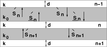
Figure 1: The up- and down-going waves near scatterer $n$. We consider a random medium consisting of thin layers, or 1D scatterers, of thickness $d$ and local wavenumber $k$ embedded in a homogeneous background medium of wavenumber $k_{0}$.

$$\left|\acute{S}_{n}\right|^{2}+\left|\grave{S}_{n+1}\right|^{2}=\left(\left|r\right|^{2}+\left|t\right|^{2}\right)\left(\left|\grave{S}_{n}\right|^{2}+\left|\acute{S}_{n+1}\right|^{2}\right)+$$

$$\left(r^{*}t+t^{*}r\right)\left(\grave{\underline{S}}_{n}^{*}\acute{S}_{n+1}+\grave{\underline{S}}_{n}\acute{S}_{n+1}^{*}\right),$$ (9)

$$\left|\acute{S}_{n}\right|^{2}-\left|\grave{S}_{n+1}\right|^{2}=\left(\left|r\right|^{2}-\left|t\right|^{2}\right)\left(\left|\grave{S}_{n}\right|^{2}-\left|\acute{S}_{n+1}\right|^{2}\right)+$$

$$\left(r^{*}t-t^{*}r\right)\left(\grave{\underline{S}}_{n}^{*}\acute{S}_{n+1}-\grave{\underline{S}}_{n}\acute{S}_{n+1}^{*}\right).$$ (10)

For a 1D scatterer embedded in a homogeneous medium, two identities exist: $|r|^{2}+|t|^{2}=1$, or conservation of energy, and $r^{*}t+t^{*}r=0$, as shown by Ursin (1983). With these identities, expressions (9) and (10) can be simplified as

$$\left|\grave{S}_{n+1}\right|^{2}-\left|\acute{S}_{n+1}\right|^{2}=\left|\grave{S}_{n}\right|^{2}-\left|\acute{S}_{n}\right|^{2},$$ (11)

$$\left(\left|\grave{S}_{n+1}\right|^{2}+\left|\acute{S}_{n+1}\right|^{2}\right)-\left(\left|\grave{S}_{n}\right|^{2}+\left|\acute{S}_{n}\right|^{2}\right)=$$

$$-2{|r|^{2}\over|t|^{2}}\left(\left|\grave{S}_{n}\right|^{2}-\left|\acute{S}_{n}\right|^{2}\right)-4{\mbox{Im}(r^{*}t)\over|t|^{2}}\mbox{Im}(\grave{\underline{S}}_{n}\acute{S}_{n+1}^{*}).$$ (12)

Note that the interference terms are not present in equation (11). This equation states that the energy flux between scatterers $n$ and $n-1$ equals that between scatterers $n$ and $n+1$. The principle of energy flux conservation in layered media has been used by Claerbout to derive the method of “acoustic daylight imaging”(Claerbout, 1985, in chapter 8). In contrast, equation (12), which describes the local change in total intensity on either side of a scatterer, contains an interference term. This term depends on the correlation between the downward propagating wavefield at the top of scatterer $n$ ($\grave{\underline{S}}_{n}$) and the upward propagating wavefield at the base of scatterer $n$ ($\acute{S}_{n+1}$).

We continue by averaging equations (11) and (12) over ensembles of randomly placed scatterers. We denote ensemble averages with brackets, $\langle\rangle$ and thus the ensemble average of the squared magnitude of the down-going wavefield between scatterers $n-1$ and $n$ by $\langle|\grave{S}_{n}|^{2}\rangle=\grave{I}_{n}$ and so on for other wavefield quantities. With ensemble averaging, we obtain from equations (11) and (12) that

$$\left(\grave{I}_{n+1}-\acute{I}_{n+1}\right)-\left(\grave{I}_{n}-\acute{I}_{n}\right)=0,$$ (13)

$$\left(\grave{I}_{n+1}+\acute{I}_{n+1}\right)-\left(\grave{I}_{n}+\acute{I}_{n}\right)=$$

$$-2{|r|^{2}\over|t|^{2}}\left(\grave{I}_{n}-\acute{I}_{n}\right)-4{\mbox{Im}(r^{*}t)\over|t|^{2}}\mbox{Im}\langle\grave{\underline{S}}_{n}\acute{S}_{n+1}^{*}\rangle.$$ (14)

The stationary 1D RT equations result from these equations by first assuming zero correlation in phase between wavefields propagating in opposite directions at scatterer $n$, $\langle\grave{\underline{S}}_{n}\acute{S}_{n+1}^{*}\rangle=0$, followed by taking a limiting procedure to move from discrete to continuous variables, as shown by Goedecke Goedecke (1977).

It is well known, however, that wave interference causes the term $\langle\grave{\underline{S}}_{n}\acute{S}_{n+1}^{*}\rangle$ to be nonzero, especially in 1D. We thus include the term containing $\langle\grave{\underline{S}}_{n}\acute{S}_{n+1}^{*}\rangle$, and therefore account for interference effects, by considering the directional wavefields on either side of a planar source within a 1D random medium. We take the depth axis ($z$-axis) positive downward. First, consider the situation above the source depth $z_{s}$. There, the up-going wavefield $\acute{\underline{S}}_{n}$ is the wavefield incident from the source direction and it can be related to the down-going wavefield $\grave{\underline{S}}_{n}$ using the reflection coefficient $R_{1}$ for the entire random medium above scatterer $n$ as Kennett (1983):

$$R_{1}\acute{\underline{S}}_{n}=\grave{\underline{S}}_{n}.$$ (15)

Moreover, the up-going wavefield $\acute{S}_{n+1}$ can be related to the up-going wavefield on the other side of scatterer $n$, $\acute{\underline{S}}_{n}$, using the reflection and transmission coefficients of a single scatterer, $r$ and $t$, and the reflection coefficient for the entire random medium below scatterer $n$, denoted $R_{2}$, as:

$$\acute{\underline{S}}_{n}={t\acute{S}_{n+1}\over 1-rR_{2}}.$$ (16)

Equations (15) and (16) relate the wavefields $\acute{S}_{n+1}$ and $\grave{\underline{S}}_{n}$:

$$\grave{\underline{S}}_{n}={R_{1}t\acute{S}_{n+1}\over 1-rR_{2}}.$$ (17)

Substituting this relationship for $\grave{\underline{S}}_{n}$ into equation (14) and assuming the ensemble averaging can be distributed as follows:

$$\mbox{Im}\langle{R_{1}t\over 1-rR_{2}}|\acute{S}_{n+1}|^{2}\rangle=\langle|\acute{S}_{n+1}|^{2}\rangle\mbox{Im}\langle{R_{1}t\over 1-rR_{2}}\rangle,$$ (18)

equation (14) above the source becomes

$$\left(\grave{I}_{n+1}+\acute{I}_{n+1}\right)-\left(\grave{I}_{n}+\acute{I}_{n}\right)=$$

$$-2{|r|^{2}\over|t|^{2}}\left(\grave{I}_{n}-\acute{I}_{n}\right)-4\acute{I}_{n+1}{\mbox{Im}(r^{*}t)\over|t|^{2}}\mbox{Im}\langle{R_{1}t\over 1-rR_{2}}\rangle.$$ (19)

Applying the same considerations to the situation below the source depth $z_{s}$ means that the direction of the wavefield incident from the source is the opposite of the case just shown. In addition, the roles of the terms $R_{1}$ and $R_{2}$ are different: $R_{1}$ is now the reflection coefficient for the entire random medium beneath scatterer $n$ and $R_{2}$ is the reflection coefficient for the entire random medium above scatterer $n$. This convention maintains the same relation between $R_{1}$ and $R_{2}$ and the direction of the incident wavefield as was used previously. Thus, starting with $R_{1}\grave{S}_{n+1}=\acute{S}_{n+1}$, equation (14) below the source is

$$\left(\grave{I}_{n+1}+\acute{I}_{n+1}\right)-\left(\grave{I}_{n}+\acute{I}_{n}\right)=$$

$$-2{|r|^{2}\over|t|^{2}}\left(\grave{I}_{n}-\acute{I}_{n}\right)-4\grave{I}_{n}{\mbox{Im}(r^{*}t)\over|t|^{2}}\mbox{Im}\langle{R_{1}^{*}t^{*}\over 1-r^{*}R_{2}^{*}}\rangle.$$ (20)

For a single realization of the ensemble, the $R_{1}$ and $R_{2}$ here are not necessarily equal to the $R_{1}$ and $R_{2}$ considered previously. However, the ensemble averages of the reflection coefficients on either side of the source are the same since the spacings of the scatterers above and below the source are drawn from the same random distribution. From equations (19) and (20), the two situations differ not only by the direction of the wavefield present in the last term ($\grave{I}_{n}$ or $\acute{I}_{n+1}$), but also by a sign change in the last term (since $\mbox{sgn}[\mbox{Im}\langle{R_{1}^{*}t^{*}\over 1-r^{*}R_{2}^{*}}\rangle]=-\mbox{sgn}[\mbox{Im}\langle{R_{1}t\over 1-rR_{2}}\rangle]$).

III Modified KM Theory: the stationary case

With these two cases (above and below the source), we now take the limiting procedure – as discussed by Goedecke Goedecke (1977) – to move from the discrete to the continuous case. We examine here the case below the source and then state the result for the case above the source, since the procedure for the two cases is the same. First, note that $\acute{I}_{n+1}$ and $\grave{I}_{n+1}$ are defined at the base of scatterer $n$, just as $\acute{I}_{n}$ and $\grave{I}_{n}$ are defined at the base of scatterer $n-1$. We define the average spacing between the scatterers as $\rho^{-1}$ and thus the number of scatterers per unit depth is $\rho$ (the number density). Multiplying both sides of equation (20) by $\rho$ results in

$${\left(\grave{I}_{n+1}+\acute{I}_{n+1}\right)-\left(\grave{I}_{n}+\acute{I}_{n}\right)\over\rho^{-1}}=$$

$$-2\rho{|r|^{2}\over|t|^{2}}\left(\grave{I}_{n}-\acute{I}_{n}\right)-4\rho\grave{I}_{n}{\mbox{Im}(r^{*}t)\over|t|^{2}}\mbox{Im}\langle{R_{1}^{*}t^{*}\over 1-r^{*}R_{2}^{*}}\rangle.$$ (21)

As pointed out by Goedecke Goedecke (1977), the term on the l.h.s. of equation (21) becomes a spatial derivative when making the transition to a continuous depth variable $n\rho^{-1}\rightarrow z$. Therefore, the directional wavefields become functions of $z$, that is, $\grave{I}_{n}=I_{d}(z)$ and $\acute{I}_{n}=I_{u}(z)$ where $I_{d}$ and $I_{u}$ are the ensemble-averaged down-going and up-going intensities. Therefore, equation (21) becomes

$${d\left(I_{d}+I_{u}\right)\over dz}=$$

$$-2\rho{|r|^{2}\over|t|^{2}}\left(I_{d}-I_{u}\right)-4\rho I_{d}{\mbox{Im}(r^{*}t)\over|t|^{2}}\mbox{Im}\langle{R_{1}^{*}t^{*}\over 1-r^{*}R_{2}^{*}}\rangle.$$ (22)

We further simplify equation (22) by defining the ensemble-averaged total intensity $I_{t}=I_{d}+I_{u}$ and the ensemble-averaged intensity flux $I_{f}=I_{d}-I_{u}$. This simplifies equation (22) as

$${dI_{t}\over dz}=-2\rho{|r|^{2}\over|t|^{2}}I_{f}-4\rho I_{d}{\mbox{Im}(r^{*}t)\over|t|^{2}}\mbox{Im}\langle{R_{1}^{*}t^{*}\over 1-r^{*}R_{2}^{*}}\rangle.$$ (23)

We finally define the scattering mean free path $\ell_{s}$, the localization length $\ell_{loc}$, and a dimensionless parameter $B$ as

$${B\over\ell_{s}} = \rho{|r|^{2}\over|t|^{2}}$$

$${1\over\ell_{loc}} = 2\rho{\mbox{Im}(r^{*}t)\over|t|^{2}}\mbox{Im}\langle{R_{1}^{*}t^{*}\over 1-r^{*}R_{2}^{*}}\rangle.$$ (24)

Using these parameters, we can rewrite equation (23) concisely as

$${dI_{t}\over dz}={-2B\over\ell_{s}}I_{f}-{2\over\ell_{loc}}I_{d}.$$ (25)

We have chosen the definitions in equation (24) in a manner consistent with the usual definitions for these quantities Goedecke (1977); Sheng (1995). For instance, regarding the quantity $\rho|r|^{2}/|t|^{2}$, in the weak scattering limit ($|t|^{2}\approx 1$) we find that

$$\rho{|r|^{2}\over|t|^{2}}\approx\rho|r|^{2}=\rho(|r|^{2}+|t-1|^{2}){|r|^{2}\over|r|^{2}+|t-1|^{2}}={B\over\ell_{s}},$$ (26)

where

$$B={|r|^{2}\over|r|^{2}+|t-1|^{2}},$$ (27)

Thus, $B$ is a dimensionless parameter describing the directionality of the scattering Haney et al. (2005). For isotropic scattering, $B=1/2$. In addition we define

$${1\over\ell_{s}}=\rho(|r|^{2}+|t-1|^{2}),$$ (28)

consistent with what we know for the 1D scattering cross section from Sheng (1995): $\sigma_{s}=|r|^{2}+|t-1|^{2}$. Therefore, from equation (28), we can identify the factor $\rho(|r|^{2}+|t-1|^{2})=\rho\sigma_{s}$. In the weak scattering limit, it is well known that $\ell_{s}=1/\rho\sigma_{s}$. Thus, our definition for $\ell_{s}$ in equation (28) is consistent with the usual definition of $\ell_{s}$ in the weak scattering limit. Appendix A demonstrates the consistency of the definition for $\ell_{loc}$ as it appears in equation (25) based on the relation in equation (24).

We have just shown how to apply the limiting procedure to equation (20). Applying the same limiting procedure to equations (13) and (19) gives all of the necessary stationary transport equations, which we summarize here:

$${dI_{f}\over dz}=0,$$ (29)

$${dI_{t}\over dz} = {-2B\over\ell_{s}}I_{f}+{2\over\ell_{loc}}I_{u}~{}~{}~{}~{}~{}\mbox{for $z<z_{s}$}$$ (30)

$$= {-2B\over\ell_{s}}I_{f}-{2\over\ell_{loc}}I_{d}~{}~{}~{}~{}~{}\mbox{for $z>z_{s}$}.$$

These equations comprise the modified KM equations in the stationary case. Equation (30) may be rewritten more concisely as

$${dI_{t}\over dz}=-2\left[{B\over\ell_{s}}+{1\over\ell_{loc}}\right]I_{f}-{\mbox{sgn}(z-z_{s})\over\ell_{loc}}(I_{t}-|I_{f}|),$$ (31)

where the quantity $I_{t}-|I_{f}|$ is either $2I_{u}$ for $z>z_{s}$ or $2I_{d}$ for $z<z_{s}$: it is twice the intensity propagating back toward the source. Equation (31) shows that the inclusion of wave interference in the KM (or RT) equations leads to two additional terms which affect the average total intensity in different ways. The first term containing $1/\ell_{loc}$ on the r.h.s. of equation (31) causes the coherent intensity to decay more rapidly than when wave interference is neglected. Furthermore, the second term containing $1/\ell_{loc}$ on the r.h.s. causes the spatial distribution of the incoherent intensity to be entirely different than in the the case of no interference (as demonstrated later in a numerical example). The form of equation (31) allows the identification of the extinction mean free path (the decay of the coherent intensity), $1/\ell_{ext}=B/\ell_{s}+1/\ell_{loc}$. This insight is possible since the quantity $I_{t}-|I_{f}|$ in equation (31) is zero for the coherent intensity. Note that the coherent intensity decays exponentially even without interference effects ($\ell_{loc}\rightarrow\infty$, or RT) due to scattering out of the forward direction.

IV Modified KM theory: the time-dependent case

Having derived the modified KM equations for the stationary case in equations (31) and (29), we will turn our attention to the time-dependent (dynamic) case. Given the current coordinate system for $z$, this is accomplished by noting that $dI_{u}/dz=\partial I_{u}/\partial z+v^{-1}\partial I_{u}/\partial t$ and $dI_{d}/dz=\partial I_{d}/\partial z-v^{-1}\partial I_{d}/\partial t$, where $v$ is the velocity of energy transport (the energy velocity). Including the presence of planar isotropic (zero net down-going component) sources Haney et al. (2005), we obtain the following time-dependent equations

$${\partial I_{f}\over\partial z}+{1\over v}{\partial I_{t}\over\partial t}={\Gamma\over v},$$ (32)

$${\partial I_{t}\over\partial z}+{1\over v}{\partial I_{f}\over\partial t}=-2\left[{B\over\ell_{s}}+{1\over\ell_{loc}}\right]I_{f}-{\mbox{sgn}(z-z_{s})\over\ell_{loc}}(I_{t}-|I_{f}|),$$ (33)

where $\Gamma$ is the isotropic (omnidirectional) source term Haney et al. (2005). Note that for $\ell_{loc}\rightarrow\infty$ (no wave interference), equations (32) and (33) are the same equations as have been studied previously by others within the context of RT in layered media Wu (1993); Wu and Xie (1994); Wu (1998); Haney et al. (2005).

With equations (32) and (33), which are the modified KM equations in the time-dependent case, we proceed to numerically solve the equations for two cases: with interference and without ($\ell_{loc}\rightarrow\infty$, or RT). These cases are compared to ensemble averages of simulations of the wave equation.

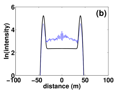
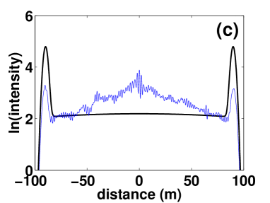
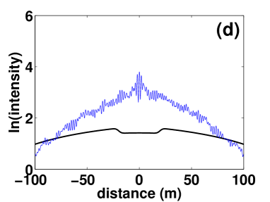
Figure 2: Comparison of numerical results for ensemble-averaged wave propagation (thin blue line) and standard KM theory, or RT (thick black line). The various panels show: (a) $t=0$ s, (b) $t=0.02$ s, (c) $t=0.045$ s, (d) $t=0.11$ s. The source time function is zero-phase and hence acausal (symmetric about $t=0$ s).

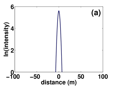
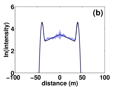
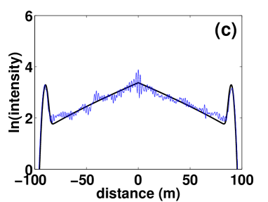
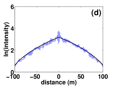
Figure 3: Comparison of numerical results for ensemble-averaged wave propagation (thin blue line) and modified KM theory (thick black line). The panels show the same times as depicted in Figure 2. The modified KM equations are seen to accurately model the exponential localization of intensity at the source position than in Figure 2.

V Numerical simulations

Our numerical solution of equations (32) and (33) exploits staggered grid finite difference methods Virieux (1986). In this technique, we calculate the total intensity $I_{t}$ and the intensity flux $I_{f}$ on different spatial grids that have been shifted by half of a grid-spacing and on different temporal grids shifted by half of a time step. Our purpose is to test whether the modified KM equations, equations (32) and (33), predict the results of a wave-based simulation. Therefore, we also simulate the wave equation for normally-incident plane waves in a layered medium, excited by a planar force source:

$${1\over c^{2}(z)}~{}{\partial^{2}u\over\partial t^{2}}-{\partial^{2}u\over\partial z^{2}}={1\over\rho c^{2}(z)}Fw(t)\delta(z),$$ (34)

where $u$ is the displacement field as a function of time $t$ and spatial coordinate $z$, $c$ is the phase velocity, $\rho$ is the density of the medium, $F$ is a dimensionless constant related to the strength of the forcing function, $w(t)$ is the dimensionless source time function, and $\delta(z)$ is the spatial delta function. We simulate equation (34) by the finite-difference method using centered, second-order approximations for the derivatives. The details of the numerical implementation have been previously discussed in Haney et al. (2005).

The setup of our numerical simulation is as follows: for a single realization, we place 50 scatterers randomly over a depth range of $L=200$ m. The scatterers are lower in propagation velocity (1000 m/s) than the background medium (2000 m/s) but have the same density. We excite a source in the center of the 200-m range at $z_{s}=0$ m. At the ends of the 200-m range are absorbing boundaries. To obtain ensemble averages of the total intensity, we first bandpass filter our numerical results from a single realization with a Gaussian filter peaked at 500 Hz. We filter in the frequency domain since the transport properties (i.e., $\ell_{s}$ and $\ell_{loc}$) are strongly dependent on frequency. In other words, equations (32) and (33) model the wave experiment in a particular frequency band. After filtering, we square the wavefield for each of 100 simulations with randomly placed scatterers and then add the squared wavefields. From the ensemble-averaged wavefields, we estimate the extinction mean free path $\ell_{ext}$ from the decay of the coherent intensity and the localization length $\ell_{loc}$ from the exponential decay of the incoherent intensity away from the source. We find $\ell_{ext}=38.1\pm 0.5$ m and $\ell_{loc}=57.2\pm 1.7$ m. These two parameters enter into equations (32) and (33). We further find that the energy velocity of the coherent wave is only slightly altered from the phase velocity of the background medium (2000 m/s), which is expected since the scatterers we employ are 1D versions of Rayleigh scatterers ($B=1/2$, with thickness $d$ much less than the dominant wavelength) Sheng (1995), and hence are not resonant scatterers.

The thick black line in Figure 2 is the total intensity from the numerical solution of the standard KM equations (RT, $\ell_{loc}\rightarrow\infty$), with the wave simulation shown as the thin blue line. Note that these snapshots are logarithmic in intensity. Strong localization effects are evident in the wave simulation as seen in the sharp exponential peak in the total intensity at the source position at later times. This behavior is not captured in the solution of the standard KM equations, which predict that the total intensity is flat around the source position. In addition, the standard KM equations significantly under-predict the decay of the coherent wave. The discrepancy between standard KM theory and the wave simulation is most evident at $t=0.11$ s in Figure 2(d), where the wave simulation shows a concentration of total intensity near the source position.

The simulation for the modified KM equations is the thick black line in Figure 3. In contrast to the standard KM equations (or RT), the modified KM equations capture the exponentially-peaked behavior of the total intensity near the source position and, at all times, agree well with the wave simulation. Thus, the modified KM equations are capable of modeling the transport of intensity in 1D localized media, where interference effects cannot be ignored. It is worth emphasizing finally that both the standard KM solution in Figure 2 and the modified KM solution in Figure 3 satisfy global energy conservation.

VI Conclusion

With a proper modification to the well known Kubelka-Munk (KM) equations, we are able to accurately describe the transport of wave intensity in a 1D layered medium at all times, even when interference effects dominate (e.g., wave localization). This is confirmed by numerical simulations comparing wave simulations and the modified Kubelka-Munk equations. In the future, we plan to extend our approach, which currently uses only two fluxes, to a theory valid for 2D and 3D disordered media. One approach to this extension would utilize higher dimensional discrete flux theories as described by Cwilich (2002). Such a transport theory will be capable of simultaneously describing the propagating coherent intensity, the intensity flux, and the localization transition in 3D.

VII Acknowledgments

We thank John Scales for many useful discussions. Partially supporting KvW are the NSF (EAR-0337379) and ARO (DAAD19-03-1-0292).

Appendix A Verification of The localization length

Here, we give credence to our use of the term localization length $\ell_{loc}$ as it appears in equation (25). By doing so, we justify the expression for $\ell_{loc}$ in equation (24). We proceed by finding the stationary transmission coefficient for a slab geometry in the case of interference. We adopt the approach shown by van Rossum and Nieuwenhuizen (1999), wherein the authors derived the stationary transmission coefficient $T$ for the case of no interference. In that case, $T(L)\approx z_{e}/L$, where $z_{e}$ is the extrapolation length outside the slab and $L$ is the thickness of the slab van Rossum and Nieuwenhuizen (1999). In analogy to electronic systems, the behavior $T(L)\approx z_{e}/L$ is an expression of Ohm’s law.

We begin by taking the stationary version of equations (32) and (33)

$${dI_{f}\over dz}={\Gamma\over v},$$ (35)

$${dI_{t}\over dz}=-2\left[{B\over\ell_{s}}+{1\over\ell_{loc}}\right]I_{f}-{\mbox{sgn}(z-z_{s})\over\ell_{loc}}(I_{t}-|I_{f}|),$$ (36)

where, as discussed before in reference to equations (32) and (33), $\Gamma$ is the isotropic (omnidirectional) source term Haney et al. (2005). Let a single stationary (planar) source act at depth $z_{s}$, such that $\Gamma=\delta(z-z_{s})$. Based on physical considerations, we know that $I_{t}$ is symmetric (even) about $z=z_{s}$ and $I_{f}$ is antisymmetric (odd). This, together with the fact that $\Gamma=\delta(z-z_{s})$ in equation (35), leads to the relation $I_{f}=\mbox{sgn}(z-z_{s})/2v$ and therefore that $\mbox{sgn}(I_{f})=\mbox{sgn}(z-z_{s})$. Since $\mbox{sgn}(I_{f})|I_{f}|=I_{f}$, equation (36) may be written as

$${dI_{t}\over dz}=-\left[{2B\over\ell_{s}}+{1\over\ell_{loc}}\right]I_{f}-{\mbox{sgn}(z-z_{s})\over\ell_{loc}}I_{t}.$$ (37)

Solving this equation for $I_{f}$ allows a substitution for $I_{f}$ in equation (35). At depths away from the source (for $z\neq z_{s}$), this gives an expression in terms of $I_{t}$ only

$${d^{2}I_{t}\over dz^{2}}+{1\over\ell_{loc}}{d\over dz}\left[\mbox{sgn}(z-z_{s})I_{t}\right]=0.$$ (38)

For the case of no interference, $\ell_{loc}\rightarrow\infty$, equation (38) reduces to the Laplace equation (the diffusion equation in the stationary case). However, when interference is taken into account, the equation is a modified Laplace equation.

In preparation for an application of the standard approach shown by van Rossum and Nieuwenhuizen (1999), we proceed by investigating how the extrapolation length outside of a slab of thickness $L$ changes when interference is accounted for. We use the well-known approach of Morse and Feshbach (1953) to define the extrapolation length. Consider a slab containing randomly located thin layers extending from $z=0$ to $z=L$. Outside of this interval, the medium is homogeneous. Take a planar source of intensity at some $z_{s}<0$, outside of the slab. Since the entire slab extends over $z=0$ to $z=L$, we have $z_{s}<z$ and thus $\mbox{sgn}(z-z_{s})=1$ for all points $z$ within the slab. In this case, equations (37) and (38) are, for all points $z$ inside of the slab, given by

$${dI_{t}\over dz}=-\left[{2B\over\ell_{s}}+{1\over\ell_{loc}}\right]I_{f}-{I_{t}\over\ell_{loc}},$$ (39)

and

$${\partial^{2}I_{t}\over\partial z^{2}}+{1\over\ell_{loc}}{\partial I_{t}\over\partial z}=0.$$ (40)

At the far end of the slab $z=L$, we require there be no up-going intensity $I_{u}=(I_{t}-I_{f})/2=0$. Now using equation (39), we substitute for $I_{f}$ in the relation $I_{t}-I_{f}=0$, giving an equation in terms of $I_{t}$ only

$$I_{t}+{\ell_{tr}\ell_{loc}\over\ell_{loc}+\ell_{tr}}\left[{dI_{t}\over dz}+{I_{t}\over\ell_{loc}}\right]=0,$$ (41)

where we use the transport mean free path $\ell_{tr}=\ell_{s}/2B$ to make the notation concise Haney et al. (2005). We can rewrite equation (41) as

$$I_{t}+\alpha{dI_{t}\over dz}=0.$$ (42)

where $\alpha=\ell_{tr}\ell_{loc}/(\ell_{loc}+2\ell_{tr})$. Equation (42) means that, near $z=L$, $I_{t}\approx C(L+\alpha-z)/\alpha$ where $C$ is a dimensioning constant. Within this approximation, $I_{t}=0$ at $z=L+\alpha$; therefore, the extrapolation length $z_{e}$ - the distance outside of the slab where $I_{t}$ vanishes - is equal to $\alpha$. That is, $z_{e}=\ell_{tr}\ell_{loc}/(\ell_{loc}+2\ell_{tr})$. One can see in this expression that, for no interference ($\ell_{loc}\rightarrow\infty$), $z_{e}=\ell_{tr}$ which is the usual extrapolation length encountered in 1D when interference is neglected Haney et al. (2005).

At the side of the slab on which the source of intensity is incident, at $z=0$, we require the down-going intensity to be equal to the incident intensity, $I_{0}$. Thus, $I_{d}=(I_{t}+I_{f})/2=I_{0}$ at $z=0$. Using equation (39), we substitute for $I_{f}$ in the relation $(I_{t}+I_{f})/2=I_{0}$, giving

$$I_{t}-{\ell_{tr}\ell_{loc}\over\ell_{loc}+\ell_{tr}}\left[{\partial I_{t}\over\partial z}+{I_{t}\over\ell_{loc}}\right]=2I_{0}.$$ (43)

Equation (43) may be rewritten as

$$I_{t}-\ell_{tr}{\partial I_{t}\over\partial z}={2I_{0}(\ell_{loc}+\ell_{tr})\over\ell_{loc}}.$$ (44)

Near $z=0$, the solution is approximately given by

$$I_{t}\approx{2I_{0}(\ell_{loc}+\ell_{tr})\over\ell_{loc}}\left[{z\over\ell_{tr}}+2\right].$$ (45)

Within this approximation, at a distance equal to the (interference adjusted) extrapolation length outside of the slab, $z=-z_{e}$, $I_{t}$ is therefore given by

$$I_{t}=2I_{0}{(\ell_{loc}+\ell_{tr})(\ell_{loc}+4\ell_{tr})\over\ell_{loc}(\ell_{loc}+2\ell_{tr})}=2I_{0}\Delta,$$ (46)

where we represent the term containing $\ell_{loc}$ and $\ell_{tr}$ by $\Delta$.

Following the method employed by van Rossum and Nieuwenhuizen (1999), we seek to solve equation (40) with the boundary conditions $I_{t}=0$ and $I_{t}=2I_{0}\Delta$ at the (interference adjusted) extrapolation lengths, $z=L+z_{e}$ and $z=-z_{e}$ respectively. The solution is

$$I_{t}(z)=2I_{0}\Delta\left[{e^{-z/\ell_{loc}}-e^{-(L+z_{e})/\ell_{loc}}\over e^{z_{e}/\ell_{loc}}-e^{-(L+z_{e})/\ell_{loc}}}\right].$$ (47)

The steady-state transmission coefficient, $T(L)=I_{t}(z=L)/I_{0}$, is

$$T(L)=2\Delta e^{-L/\ell_{loc}}\left[{1-e^{-z_{e}/\ell_{loc}}\over e^{z_{e}/\ell_{loc}}-e^{-(L+z_{e})/\ell_{loc}}}\right]\approx$$

$$2\Delta e^{-L/\ell_{loc}}\left[{1-e^{-z_{e}/\ell_{loc}}\over e^{z_{e}/\ell_{loc}}}\right].$$ (48)

where the approximation is for $z_{e}\ll L$. This expression shows that when interference is taken into account the steady-state transmission coefficient goes down exponentially as a function of the length of the slab $L$ - a hallmark of localization in the stationary case. This behavior is in stark contrast to $T(L)\approx z_{e}/L$ van Rossum and Nieuwenhuizen (1999) obtained when interference is neglected ($\ell_{loc}\rightarrow\infty$). The fact that the length scale controlling the exponential decay with $L$ in equation (48) is $\ell_{loc}$ supports the use of this term in equation (25) and, as a consequence, the expression for $\ell_{loc}$ in equation (24).

References

- Kubelka and Munk (1931) P. Kubelka and F. Munk, Zeitschrift für Technische Physik 12, 593 (1931).
- Goedecke (1977) G. H. Goedecke, Journal of the Optical Society of America 67, 1339 (1977).
- Sheng (1995) P. Sheng, Introduction to wave scattering, localization, and mesoscopic phenomena (Academic Press, San Diego, 1995).
- Papanicolaou (1998) G. Papanicolaou, Documenta Mathematica, Extra Volume ICM pp. 1–23 (1998).
- Haney and Snieder (2003) M. Haney and R. K. Snieder, Physical Review Letters 91, 093902 (2003).
- White et al. (1987) B. White, P. Sheng, Z.-Q. Zhang, and G. Papanicolaou, Physical Review Letters 59, 1918 (1987).
- Berry and Klein (1997) M. V. Berry and S. Klein, European Journal of Physics 18, 222 (1997).
- Shapira and Fischer (2005) O. Shapira and B. Fischer, Journal of the Optical Society of America B 22, 2542 (2005).
- Vollhardt and Wolfle (1992) D. Vollhardt and P. Wolfle, in Electronic Phase Transitions, edited by W. Hanke and Y. Kopaev (Elsevier, Amsterdam, 1992), pp. 1–78.
- Friedrich and Wegler (2005) C. Friedrich and U. Wegler, Geophysical Research Letters 32, L14312 (2005).
- Hemmer (1961) P. C. Hemmer, Physica A 27, 79 (1961).
- Paasschens (1997) J. C. Paasschens, Physical Review E 56, 1135 (1997).
- Wu (1993) R.-S. Wu, in 63th Ann. Internat. Mtg., Society of Exploration Geophysicists, Expanded Abstracts (1993), pp. 1014–1017.
- Wu (1998) R.-S. Wu, in Wave propagation in complex media, edited by G. Papanicolaou (Springer, New York, 1998), pp. 273–288.
- Wu and Xie (1994) R.-S. Wu and X.-B. Xie, in 64th Ann. Internat. Mtg., Society of Exploration Geophysicists, Expanded Abstracts (1994), pp. 1302–1305.
- Sato and Fehler (1998) H. Sato and M. Fehler, Seismic wave propagation and scattering in the heterogeneous earth (Springer-Verlag, New York, 1998).
- Sato (1993) H. Sato, Geophysical Journal International 112, 141 (1993).
- Haney et al. (2005) M. M. Haney, K. van Wijk, and R. K. Snieder, Geophysics 70(1), T1 (2005).
- Bakut et al. (2003) P. A. Bakut, O. M. Ershova, and Y. P. Shumilov, Geophysical Journal International 155, 391 (2003).
- Baluni and Willemsen (1985) V. Baluni and J. Willemsen, Physical Review A 31, 3358 (1985).
- Scales and Vleck (1997) J. A. Scales and E. S. V. Vleck, Journal of Computational Physics 133, 27 (1997).
- van der Baan (2001) M. van der Baan, Geophysical Journal International 145, 631 (2001).
- Shapiro and Hubral (1999) S. A. Shapiro and P. Hubral, Elastic Waves in Random Media - Fundamentals of Seismic Stratigraphic Filtering (Springer-Verlag, Berlin, 1999).
- Lobkis and Weaver (2005) O. I. Lobkis and R. L. Weaver, Physical Review E 71(1), 011112 (pages 8) (2005).
- Claerbout (1985) J. F. Claerbout, Fundamentals of Geophysical Data Processing (Blackwell Scientific, Palo Alto, CA, 1985).
- Ursin (1983) B. Ursin, Geophysics 48, 1063 (1983).
- Kennett (1983) B. L. N. Kennett, Seismic wave propagation in stratified media (Cambridge University Press, Cambridge, 1983).
- Virieux (1986) J. Virieux, Geophysics 51, 889 (1986).
- Cwilich (2002) G. A. Cwilich, Nanotechnology 13, 274 (2002).
- van Rossum and Nieuwenhuizen (1999) M. van Rossum and T. Nieuwenhuizen, Reviews of Modern Physics 71, 313 (1999).
- Morse and Feshbach (1953) P. Morse and H. Feshbach, Methods of theoretical physics (McGraw-Hill, New York, 1953).