Proposal for detection of non-Markovian decay via current noise

Abstract

We propose to detect non-Markovian decay of an exciton qubit coupled to multi-mode bosonic reservoir via shot-noise measurements. Non-equilibrium current noise is calculated for a quantum dot embedded inside a p-i-n junction. An additional term from non-Markovian effect is obtained in the derivation of noise spectrum. As examples, two practical photonic reservoirs, photon vacuum with the inclusion of cut-off frequency and surface plasmons, are given to show that the noise may become super-Poissonian due to this non-Markovian effect. Utilizing the property of super-radiance is further suggested to enhance the noise value.

Introduction.–Due to rapid progress of quantum information science, great attention has been focused on the dynamics of systems interacting with their surroundings. Radiative decay of a two-level atom maybe one of the most obvious examples in this issue and can be traced back to such early works as that of Albert Einstein in 1917. 1 While Markovian approximation is widely adopted to treat decoherence and relaxation problems, non-Markovian dynamics of qubit systems have attracted increasing attention lately. 2

Turning to solid state systems, an exciton in a quantum dot (QD) can be viewed as a two-level system. Radiative properties of QD excitons, such as super-radiance 3 and Purcell effect 4 , have attracted great attention during the past two decades. Utilizing QD excitons for quantum gate operations have also been demonstrated experimentally. 5 With the advances of fabrication technologies, it is now possible to embed QDs inside a p-i-n structure 6 , such that the electron and hole can be injected separately from opposite sides. This allows one to examine the exciton dynamics in a QD via electrical currents 7 .

Recently, the interest in measurements of shot noise in quantum transport has risen owing to the possibility of extracting valuable information not available in conventional dc transport experiments 8 . In this work, we propose to detect non-Markovian decay of a exciton qubit via the current noise of a QD p-i-n junction. Without making Markovian approximation to the exciton-boson interaction, we analytically show that the Fano factor (zero-frequency noise) may become super-Poissonian. As examples, two practical photonic environments, photon vacuum with the inclusion of cut-off frequency and surface plasmons, are given to show this non-Markovian effect. To enhance the noise value, we further suggest utilizing the property of super-radiance.

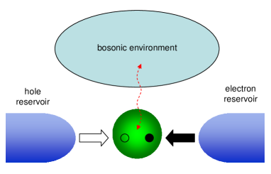
Figure 1: (Color online) Schematic view of a QD p-i-n junction with its exciton coupled to a bosonic environment.

The model.–QDs can now be embedded in a p-i-n junction, such that many applications can be accomplished by electrical control. As shown in Fig. 1, we wish to see non-Markovian effect between the system and reservoir via measurements of electrical currents. For simplicity, both the hole and electron reservoirs of the p-i-n junction are assumed to be in thermal equilibrium. For the physical phenomena we are interested in, the Fermi level of the p(n)-side hole (electron) is slightly lower (higher) than the hole (electron) subband in the dot. After a hole is injected into the hole subband in the QD, the n-side electron can tunnel into the exciton level because of the Coulomb interaction between the electron and hole. Thus, we may introduce the three dot states: $\left|0\right\rangle=\left|0,h\right\rangle$, $\left|\uparrow\right\rangle=\left|e,h\right\rangle$, and $\left|\downarrow\right\rangle=\left|0,0\right\rangle$, where $\left|0,h\right\rangle$ means there is one hole in the QD, $\left|e,h\right\rangle$ is the exciton state, and $\left|0,0\right\rangle$ represents the ground state with no hole and electron in the QD. One might argue that one can not neglect the state $\left|e,0\right\rangle$ for real devices since the tunable variable is the applied voltage. This can be resolved by fabricating a thicker barrier on the electron side so that there is little chance for an electron to tunnel in advance 7 . Thus, the couplings of the dot states to the electron and hole reservoirs are to be described by the standard tunnel Hamiltonian

$$H_{T}=\sum_{\mathbf{q}}(V_{\mathbf{q}}c_{\mathbf{q}}^{\dagger}\left|0\right\rangle\left\langle\uparrow\right|+W_{\mathbf{q}}d_{\mathbf{q}}^{\dagger}\left|0\right\rangle\left\langle\downarrow\right|+H.c.),$$ (1)

where $c_{\mathbf{q}}$ and $d_{\mathbf{q}}$ are the electron operators in the right and left reservoirs, respectively. $V_{\mathbf{q}}$ and $W_{\mathbf{q}}$ couple the channels $\mathbf{q}$ of the electron and the hole reservoirs. The interaction between the exciton qubit and its bosonic environment is written as

$$H_{ex-bosonic} = \sum_{k}D_{k}b_{k}^{\dagger}\left|\downarrow\right\rangle\left\langle\uparrow\right|+H.c.$$ (2)

$$= \left|\downarrow\right\rangle\left\langle\uparrow\right|X+\left|\uparrow\right\rangle\left\langle\downarrow\right|X^{\dagger},$$

where $X=\sum_{k}D_{k}b_{k}^{\dagger}$, $b_{k}^{\dagger}$ denotes the creation operator of the bosonic reservoir, and $D_{k}$ describes the system-reservoir coupling.

With Eqs. (1) and (2), one can now write down the equation of motion for the reduced density operator

$$\frac{d}{dt}\rho(t) = -Tr_{res}\int_{0}^{t}dt^{\prime}[H_{T}(t)+H_{ex-bosonic}(t),$$ (3)

$$[H_{T}(t^{\prime})+H_{ex-bosonic}(t^{\prime}),\widetilde{\Xi}(t^{\prime})]],$$

where $\widetilde{\Xi}(t^{\prime})$ is the total density operator. Note that the trace in Eq. (3) is taken with respect to both bosonic and electronic reservoirs. If the couplings to the electron and hole reservoirs are weak, it is reasonable to assume that the standard Born-Markov approximation with respect to the electronic couplings is valid. In this case, multiplying Eq. (3) by $\overset{\wedge}{n_{\uparrow}}=\left|\uparrow\right\rangle\left\langle\uparrow\right|$ and $\overset{\wedge}{n_{\downarrow}}=\left|\downarrow\right\rangle\left\langle\downarrow\right|$, the equations of motions can be written as

$$\frac{\partial}{\partial t}\binom{\overset{\wedge}{\left\langle n_{\uparrow}\right\rangle}_{t}}{\overset{\wedge}{\left\langle n_{\downarrow}\right\rangle}_{t}} = \int dt^{\prime}\binom{-A(t-t^{\prime})\overset{\wedge}{\left\langle n_{\uparrow}\right\rangle}_{t^{\prime}}}{A(t-t^{\prime})\overset{\wedge}{\left\langle n_{\downarrow}\right\rangle}_{t^{\prime}}}$$ (6)

$$+\left[\begin{array}[]{cc}-\Gamma_{L}&-\Gamma_{L}\\ 0&-\Gamma_{R}\end{array}\right]\binom{\overset{\wedge}{\left\langle n_{\uparrow}\right\rangle}_{t}}{\overset{\wedge}{\left\langle n_{\downarrow}\right\rangle}_{t}}+\binom{\Gamma_{L}}{0},$$

where $\Gamma_{L}$ $=2\pi\sum_{\mathbf{q}}V_{\mathbf{q}}^{2}\delta(\varepsilon_{\uparrow}-\varepsilon_{\mathbf{q}}^{\uparrow})$ , $\Gamma_{R}=2\pi\sum_{\mathbf{q}}W_{\mathbf{q}}^{2}\delta(\varepsilon_{\downarrow}-\varepsilon_{\mathbf{q}}^{\downarrow})$, and $\varepsilon=\hbar\omega_{0}=\varepsilon_{\uparrow}-\varepsilon_{\downarrow}$ is the energy gap of the QD exciton. Here, $A(t-t^{\prime})\equiv C(t-t^{\prime})+C^{\ast}(t-t^{\prime})$ can be viewed as the (bosonic) reservoir correlation function with the function $C$  defined as $C(t-t^{\prime})$ $\equiv\left\langle X_{t}X_{t^{\prime}}^{\dagger}\right\rangle_{0}$. The appearance of the two-time correlation is attributed to that in the derivation of Eq. (4), we only assume the Born approximation to the bosonic reservoir, i.e. the Markovian one is not made.

One can now define the Laplace transformation for real $z,$

$$C_{\varepsilon}(z) \equiv \int_{0}^{\infty}dte^{-zt}e^{i\varepsilon t}C(t)$$

$$n_{\uparrow}(z) \equiv \int_{0}^{\infty}dte^{-zt}\overset{\wedge}{\left\langle n_{\uparrow}\right\rangle}_{t}\text{ \ }etc.,\text{ }z>0$$ (7)

and transform the whole equations of motion into $z$-space,

$$n_{\uparrow}(z) = -A_{\varepsilon}(z)n_{\uparrow}(z)/z+\frac{\Gamma_{L}}{z}[1/z-n_{\uparrow}(z)-n_{\downarrow}(z)],$$

$$n_{\downarrow}(z) = A_{\varepsilon}(z)n_{\downarrow}(z)/z-\frac{\Gamma_{R}}{z}n_{\downarrow}(z).$$ (8)

These equations can then be solved algebraically, and the tunnel current from the hole–side barrier, $\overset{\wedge}{I}_{R}=-e\Gamma_{R}\overset{\wedge}{\left\langle n_{\downarrow}\right\rangle}_{t}$, can in principle be obtained by performing the inverse Laplace transformation. Depending on the complexity of the correlation function $C(t-t^{\prime})$ in the time domain, this can be a formidable task which can however be avoided if one directly seeks the quantum noise.

In a quantum conductor in nonequilibrium, electronic current noise originates from the dynamical fluctuations of the current around its average. To study correlations between carriers, we relate the exciton dynamics with the hole reservoir operators by introducing the degree of freedom $n$ as the number of holes that have tunneled through the hole-side barrier, and write

$$\overset{\cdot}{n}_{0}^{(n)}(t)=-\Gamma_{L}n_{0}^{(n)}(t)+\Gamma_{R}n_{\downarrow}^{(n-1)}(t),$$

$$\overset{\cdot}{n}_{\uparrow}^{(n)}(t)+\overset{\cdot}{n}_{\downarrow}^{(n)}(t)=(\Gamma_{L}-\Gamma_{R})n_{0}^{(n)}(t).$$ (9)

Eqs. (7) allow us to calculate the particle current and the noise spectrum from $P_{n}(t)=n_{0}^{(n)}(t)+n_{\uparrow}^{(n)}(t)+n_{\downarrow}^{(n)}(t)$ which gives the total probability of finding $n$ electrons in the collector by time $t$. In particular, the noise spectrum $S_{I_{R}}$ can be calculated via the MacDonald formula 9 ; 10 ,

$$S_{I_{R}}(\omega)=2\omega e^{2}\int_{0}^{\infty}dt\sin(\omega t)\frac{d}{dt}[\left\langle n^{2}(t)\right\rangle-(t\left\langle I\right\rangle)^{2}],$$ (10)

where $\frac{d}{dt}\left\langle n^{2}(t)\right\rangle=\sum_{n}n^{2}\overset{\cdot}{P_{n}}(t)$. With the help of counting statistics 10 , one can obtain

$$S_{I_{R}}(\omega)=2eI\{1+$$ (11)

$$\Gamma_{R}[\frac{A(i\omega)\Gamma_{L}}{-A(i\omega)\Gamma_{L}\Gamma_{R}+(A(i\omega)+i\omega)(\Gamma_{L}+i\omega)(\Gamma_{R}+i\omega)}+$$

$$\frac{A(-i\omega)\Gamma_{L}}{-A(-i\omega)\Gamma_{L}\Gamma_{R}+(A(-i\omega)-i\omega)(\Gamma_{L}-i\omega)(\Gamma_{R}-i\omega)}]\},$$

where $A(z)\equiv C_{\varepsilon}(z)+C_{\varepsilon}^{\ast}(z)$.

As can be seen from Eq. (9), the noise spectrum indeed contains the information of memory effect, i.e. $A(i\omega)$ and $A(-i\omega)$. However, it is not easy to see how it affects the noise. We thus take the zero-frequency limit ($\omega\rightarrow 0$), and an analytical solution with physical meaning is obtained:

$$F =S_{I_{R}}(\omega=0)/2e\left\langle I\right\rangle$$

$$=1-\frac{2\Gamma_{L}\Gamma_{R}[Re[A(0)]\Gamma_{L}+Re[A(0)](Re[A(0)]+\Gamma_{R})]}{[Re[A(0)]\Gamma_{R}+\Gamma_{L}(Re[A(0)]+\Gamma_{R})]^{2}}$$

$$+\frac{2Im[\frac{\partial A(\emph{iw})}{\partial\emph{w}}|_{\emph{w}=0}]\Gamma_{L}^{2}\Gamma_{R}^{2}}{[Re[A(0)]\Gamma_{R}+\Gamma_{L}(Re[A(0)]+\Gamma_{R})]^{2}}.$$ (12)

If one makes Markovian approximation to the bosonic reservoir, the third term in Eq. (10) vanishes and the Fano factor ($F$) is further reduced to usual sub-Poissonian result. The question here is that whether this additional term is positive or not, such that the noise feature may become super-Poissonian. To answer this, let us now consider real bosonic environments.

Surface plasmons.–The collective motions of an electron gas in a metal or semiconductor are known as the plasma oscillations. The non-vanishing divergence of the electric field $\overrightarrow{E}$, $\nabla\cdot\overrightarrow{E}\neq 0$, in the bulk material gives rise to the well known bulk plasma modes, characterized by the plasma frequency $\omega_{p}=(4\pi n_{0}e^{2}/m)^{1/2}$, where $m$ and $e$ are the electronic mass and charge and $n_{0}$ is the electron density. In the presence of surface, however, the situation becomes more complicated. Not only the bulk modes are modified, but also the surface modes can be created. 11 Like the bulk modes, surface plasmons can be excited by incident electrons or photons. 12 Many works were devoted to the study of radiative decay into surface plasmons. 13 Recently, it is now possible to fabricate QDs evanescently coupled to surface plasmons, such that enhanced fluorescence are observed. 14 Based on these new developments, it is plausible to assume that the QD p-i-n junction is close to a metal surface. This allows one to examine non-Markovian effect from surface plasmons.

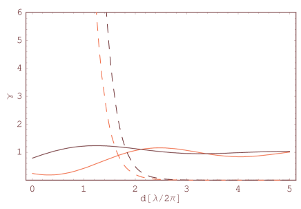
Figure 2: (Color online) Radiative decay rate of QD exciton in front of a silver surface with distance $d$ (in units of $\lambda/2\pi$, where $\lambda$ is the wavelength of the emitted photon). The plasma oscillation energy $\hbar\omega_{p}$ of silver and exciton bandgap energy $\hbar\omega_{0}$ are $3.76eV$ and $1.39eV$ 6 , respectively. The black dashed (solid) line represents the decay into the surface plasmons (photons) as the exciton dipole moment $\overset{\wedge}{p}$ is oriented perpendicular to the surface. The red lines are the case for $\overset{\wedge}{p}$ parallel to the surface.

When a semiconductor QD is near a metal surface, the vector potential to the QD exciton can be decomposed into contributions from s- and p-polarized photons and surface plasmons 15 :

$$A(\overrightarrow{r},t)=A^{s}(\overrightarrow{r},t)+A^{p}(\overrightarrow{r},t)+A_{sp}(\overrightarrow{r},t).$$ (13)

Fig. 2 shows the corresponding radiative decay rates of a QD exciton in front of a silver surface. It is evident that at short distances radiative decay is dominated by surface plasmons. Since we are interested in the effect from surface plasmons, we thus keep QD in this regime, and consider only the interaction from surface plasmons:

$$H_{ex-sp} = \sum_{\mathbf{k}}(\frac{4\pi\omega_{k}^{2}}{\hbar Acp_{k}})^{1/2}[\left|\uparrow\right\rangle\left\langle\downarrow\right|(\overset{\wedge}{k}\cdot\overset{\wedge}{p}+i\frac{k}{\nu_{0}}\cdot\overset{\wedge}{p})a_{k}e^{i\mathbf{k\cdot\rho}-\nu_{0}z}$$ (14)

$$+H.c.].$$

Here, we have chosen cylindrical coordinates $\overrightarrow{r}=(\overrightarrow{\rho},z)$ in the half-space $z\geq 0$; $\overrightarrow{k}$ is a two dimensional wave vector in the metal surface of area $A$. $a_{k}$ is the annihilation operator of surface plasmon and $\overset{\wedge}{p}$ is the transition dipole moment. The surface-plasmon frequency $\omega_{k}$ and the parameters, $\nu_{0}$ and $p_{k}$, are given by

$$\omega_{k}^{2} = \frac{1}{2}\omega_{p}^{2}+ck^{2}-(\frac{1}{4}\omega_{p}^{4}+c^{2}k^{4})^{1/2};\nu_{0}=k^{2}-\omega_{k}^{2}/c^{2};$$

$$p_{k} = \frac{\epsilon^{4}(\omega_{k})-1}{[-\epsilon(\omega_{0})-1]^{1/2}}\frac{1}{\epsilon^{2}(\omega_{k})},$$ (15)

where $\epsilon(\omega_{k})=1-$ $\omega_{p}^{2}/\omega_{k}^{2}$ is the dielectric function of the metal. By replacing $H_{ex-bosonic}$ with $H_{ex-sp}$, one can go through the procedure to obtain the current noise.

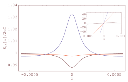
Figure 3: (Color online) Shot-noise spectrums of QD excitons in front of a silver surface.  The black, red, and blue lines represent the results of various dot-surface distances: $d=0.1,$ $0.045$, and $0.03$ (in units of $\lambda/2\pi\approx 1423\overset{\circ}{A})$, respectively. The inset shows the corresponding curves of the imaginary part of $A(i\omega)$.

The shot-noise spectrum of InAs QD excitons is numerically displayed in Fig. 3, where the tunneling rates, $\Gamma_{L}$ and $\Gamma_{R}$, are assumed to be equal to $10^{-4}\omega_{0}$ and $10^{-3}\omega_{0}$, respectively. The plasma oscillation energy $\hbar\omega_{p}$ of silver and exciton bandgap energy $\hbar\omega_{0}$ are $3.76eV$ and $1.39eV$. One knows from Fig. 2 that there is no essential difference in physics for different orientations of the exciton dipole moment. Therefore, in plotting the figure the dipole moment $\overset{\wedge}{p}$ is assumed to be along $\overset{\wedge}{z}$ direction for simplicity. Without making Markovian approximation, the black, red, and blue lines represent the results for different dot-surface distances: $d=0.1$, $0.045$, and $0.03$ (in unit of $\lambda/2\pi\approx 1423\overset{\circ}{A}$), respectively. As seen, the Fano factor gradually changes from sub-Poissonian noise to super-Poissonian one as the QD is moving toward the surface. This proves that the additional term in Eq. (10) can change the noise feature. The inset of Fig. 3 numerically shows the imaginary part of $A(i\omega)$. As the QD is closer to the silver surface, the slope becomes steeper, which coincides with the analytical result of Eq. (10).

Reasons for super-Poissonian noise actually depend on the details of the device structures. For examples, positive correlations due to resonant tunneling states 16 , noise enhancement due to quantum entanglement 17 , spin-flip co-tunneling processes 18 , non-Markovian coupling between dot and leads 19 , and quantum shuttle effect 20 . The underlying physical picture in our case maybe similar to a recent work by Djuric et al. 21 They considered the tunneling problem through a QD connected coherently to a nearby single-level dot, which is not connected to the left and right leads. In this case, the coherent hopping to the nearby dot also gives an extra ”positive” term to the Fano factor. The explanation is that the coming electron can either tunnel out of the original dot directly, or travel to the nearby dot and come back again. This indirect path is the origin of the super-Poissonian noise. In our case, as the exciton decays into surface plasmon, the non-Markovian effect from the plasmon reservoir may re-excite it now and then, such that the Fano factor is enhanced. One notes that this kind of enhancement due to quantum coherence has recently been observed in the tunneling through a stack of coupled quantum dots 22 and explained theoretically 23 .

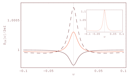
Figure 4: (Color online) Shot-noise spectrums of QD excitons in the presence of Lorentzian cutoff.  Sub-Poissonian noise represented by the black line is the result of Markovian approximation. Super-Poissonian noise (red and dashed lines) is the consequence of non-Markovian effect. To plot the figure, the exciton spontaneous lifetime ($=1/\gamma$) used here is $1.3ns$, and the cutoff frequency for red (dashed) line is $9\times 10^{16}$ $(1.2\times 10^{17})Hz$. Inset: Noise increased by the enhancemet of the effective dipole moment (400 times) via super-radiance.

The cutoff frequency.–To see whether this non-Markovian effect is general, let us return to the old quantum electrodynamic (QED) problem: spontaneous emission. Under Markovian approximation, the emission rate of a two-level atom in free space can be easily obtained via the Fermi’s Golden rule and is give by $\gamma=2\pi\sum_{\mathbf{q}}$ $\left|D_{\mathbf{q}}\right|^{2}\delta(\omega_{0}-c\left|\mathbf{q}\right|)$, where $D_{\mathbf{q}}$ is the atom-reservoir coupling strength. It’s frequency counterpart is written as $\Delta\omega=$ $\mathcal{P}\int d\mathbf{q}$ $\left|D_{\mathbf{q}}\right|^{2}/(\omega_{0}-c\left|\mathbf{q}\right|),$ where $\mathcal{P}$ denotes the principal integral. To remove the divergent problem from the integration, one can, for example, include the concept of cutoff frequency to renormalize the frequency shift. 24 In this case, the exciton-photon coupling is described by the Hamiltonian:

$$H_{ex-Ph}=\sum_{k}\frac{1}{(1+(\omega_{k}/\omega_{B})^{2})^{2}}D_{k}b_{k}^{\dagger}\left|\downarrow\right\rangle\left\langle\uparrow\right|+H.c.,$$ (16)

where the introduced Lorentzian cutoff contains the nonrelativistic cutoff frequency $\omega_{B}\approx c/a_{B}$, with $a_{B}$ being the effective Bohr radius of the exciton. 25 Replacing $H_{ex-bosonic}$ by $H_{ex-Ph}$, one can obtain the corresponding noise spectrum straightforwardly. As shown in Fig. 4, the Fano factor is sub-Poissonian (black line) under Markovian approximation, while it may become super-Poissonian (as shown by the dashed and red lines) with the consideration of non-Markovian effect from the Lorentzian cutoff.

One also finds that the magnitude of the Fano factor depends on the cutoff frequency $\omega_{B}$. With the increasing of $\omega_{B}$, the Fano factor becomes lager (the dashed line). This phenomenon allows one to examine the cutoff frequency in QED. However, one might argue that the value of the super-Poissonian noise is extremely small and may not be observable in real experiments. To overcome this obstacle, we suggest making use of the property of collective decay (super-radiance). 26 For example, one can, instead of the QD, insert a quantum well (QW) into the p-i-n junction. The interaction between the (two-dimensional) QW exciton and the photon can be written as 27

$$H^{\prime} = \sum_{\mathbf{q}nm}\sum_{k_{z}}\frac{1}{(1+(\omega_{k}/\omega_{B})^{2})^{2}}\frac{e}{m_{0}c}\sqrt{\frac{2\pi\hbar c}{(\mathbf{q}^{2}+k_{z}^{2}\mathbf{)}^{1/2}v}}$$ (17)

$$\times(\mathbf{\epsilon}_{\mathbf{q}k_{z}}\cdot\mathbf{A}_{\mathbf{q}nm})b_{\mathbf{q}k_{z}}c_{\mathbf{q}nm}^{\dagger}+\mathbf{h.c.},$$

where

$$\mathbf{A}_{\mathbf{q}nm}=\sqrt{N}\sum_{\mathbf{\rho}}F_{nm}^{\ast}(\mathbf{\rho})\int d^{2}\mathbf{\tau}w_{c}^{\ast}(\mathbf{\tau}-\mathbf{\rho})(-i\hbar\mathbf{\nabla})w_{v}(\mathbf{\tau})\text{.}$$ (18)

Here, $c_{\mathbf{q}}^{\dagger}$ and $b_{\mathbf{q}k_{z}}$ stand for the exciton and photon operators. $\mathbf{\epsilon}_{\mathbf{q}k_{z}}$ is the polarization vector of the photon. $F_{nm}(\mathbf{\rho})$ is the two-dimensional hydrogenic wavefunction of the exciton with quantum number $n$ and $m$. $w_{c}(\mathbf{\tau})$ and $w_{v}(\mathbf{\tau})$ are, respectively, the Wannier functions for the conduction band and the valence band.

With the Hamiltonian in Eq. (15), the radiative decay rate of the QW exciton can be obtained straightforwardly

$$\gamma_{\mathbf{q}nm}\sim\gamma_{0}(\lambda/d)^{2},$$ (19)

where $\gamma_{0}$ is the decay rate of a lone exciton, $\lambda$ is the wavelength of the emitted photon, and $d$ is the lattice constant of the material. The enhanced rate in Eq. (17) implies the coherent contributions from the lattice atoms within half a wavelength or so. In another word, one can say that the effective dipole moment of the QW exciton is enhanced by a factor of $(\lambda/d)^{2}$ 27 . From Eq. (10), Fig. 2, and inset of Fig. 3, we know that an enhanced rate somehow implies a larger Fano factor. Consider the real experimental values 28 , the observed enhancement is around several hundred times the lone exciton. We thus plot the Fano factor in the inset of Fig. 4. As can be seen, the value of super-Poissonian noise is greatly enhanced by super-radiance. This gives a better chance to observe the mentioned effect. Another possible candidate for the enhancement is the uniform QD-arrays. 29 Within the collective decay area defined by $\lambda^{2}$, the effective dipole moment may also be enhanced by a factor of $(\lambda/r)^{2}$ , where $r$ is the dot-lattice constant.

Finally, we note that recent advances in fabrication nanotechnologies have made it possible to grow high quality nanowires 30 , in which cavity QED phenomena can be revealed via surface plasmons. 31 It is likely that similar effects will appear if the QD p-i-n junction is coupled to the channel plasmons. Even more, since the dispersion relation in cylindrical interface is much more complex (for example, it contains both real and virtual modes 32 ), the corresponding shot-noise spectrums are expected to give more information about the non-Markovian effect. Further investigations in this direction certainly put such a system more useful in the fields of quantum transport and cavity QED.

We would like to thank Prof. T. Brandes and Prof. E. Schöll at Technische Universität Berlin, Prof. J. Y. Hsu, and Prof. S. H. Chang at Institute Electro-Optical Engineering for helpful discussions. This work is supported partially by the National Science Council, Taiwan under the grant number NSC 95-2112-M-006-031-MY3.

References

- (1) A. Einstein, Phys. Z. 18, 121 (1917).
- (2) R. Alicki, M. Horodecki, P. Horodecki, R. Horodecki, L. Jacak, and P. Machnikowski, Phys. Rev. A 70, 010501(R) (2004); S. Shresta, C. Anastopoulos, A. Dragulescu, and B. L. Hu, Phys. Rev. A 71, 022109 (2005); M. Thorwart, J. Eckel, and E. R. Mucciolo, Phys. Rev. B 72, 235320 (2005); T. Kishimoto, A. Hasegawa, Y. Mitsumori, J. Ishi-Hayase, M. Sasaki, and F. Minami, Phys. Rev. B 74, 073202 (2006).
- (3) E. Hanamura, Phys. Rev. B 38, 1228 (1988); Y. N. Chen, D. S. Chuu, and T. Brandes, Phys. Rev. Lett. 90, 166802 (2003).
- (4) J. M. Gerard, B. Sermage, B. Gayral, B. Legrand, E. Costard, and V. Thierry-Mieg, Phys. Rev. Lett. 81, 1110 (1998); G. S. Solomon, M. Pelton, and Y. Yamamoto, Phys. Rev. Lett. 86, 3903 (2001).
- (5) X. Q. Li, Y. W. Wu, D. Steel, D. Gammon, T. H. Stievater, D. S. Katzer, D. Park, C. Piermarocchi, and L. J. Sham, Science 301, 809 (2003).
- (6) Z. Yuan, B. E. Kardynal, R.M. Stevenson, A. J. Shields, C. J. Lobo, K. Cooper, N. S. Beattie, D. A. Ritchie, and M. Pepper, Science 295, 102 (2002).
- (7) Y. N. Chen and D. S. Chuu, Phys. Rev. B 66, 165316 (2002); Y. N. Chen, D. S. Chuu, and T. Brandes, Phys. Rev. B 72, 153312 (2005).
- (8) C. W. J. Beenakker, Rev. Mod. Phys. 69, 731 (1997); Y. M. Blanter and M. Buttiker, Phys. Rep. 336, 1 (2000).
- (9) D. K. C. MacDonald, Rep. Prog. Phys. 12, 56 (1948).
- (10) R. Aguado and T. Brandes, Phys. Rev. Lett. 92, 206601 (2004).
- (11) R. H. Ritchie, Phys. Rev. 106, 874 (1957).
- (12) Electromagnetic Surface Modes, edited by A. D. Boardman (John Wiley & Sons, 1982).
- (13) H. Morawitz and M. R. Philpott, Phys. Rev. B 10, 4863 (1974); M. Babiker and G. Barton, J. Phys. A: Math. Gen. 9, 129 (1976); R. Bonifacio and H. Morawitz, Phys. Rev. Lett. 36, 1559 (1976).
- (14) J. Zhang, Y. H. Ye, X. Wang, P. Rochon, and M. Xiao, Phys. Rev. B 72, 201306(R) (2005); P. P. Pompa, L. Martiradonna, A. Della Torre, F. Della Sala, L. Manna, M. De Vittorio, F. Calabi, R. Cingolani, and R. Rinaldi, Nature Nanotechnology 1, 126 (2006).
- (15) J. M. Elson and R. H. Ritchie, Phys. Rev. B 4, 4129 (1971).
- (16) Y. Chen and R. A. Webb, Phys. Rev. Lett. 97, 066604 (2006).
- (17) Y. N. Chen, T. Brandes, C. M. Li, and D. S. Chuu, Phys. Rev. B 69, 245323 (2004).
- (18) A. Thielmann, M. H. Hettler, J. König, G. Schön, Phys. Rev. Lett. 95, 146806 (2005).
- (19) H. -A. Engel and D. Loss, Phys. Rev. Lett. 93, 136602 (2004).
- (20) T. Novotny, A. Donarini, C. Flindt, and A.-P. Jauho, Phys. Rev. Lett. 92, 248302 (2004).
- (21) I. Djurica, B. Dong, and H. L. Cui, Appl. Phys. Lett. 87, 032105 (2005).
- (22) P. Barthold, F. Hohls, N. Maire, K. Pierz, and R. J. Haug , Phys. Rev. Lett. 96, 246804 (2006).
- (23) G. Kießlich, E. Schöll, T. Brandes, F. Hohls, R. J. Haug, arXiv:0706.1737 (2007).
- (24) H. E. Moses, Phys. Rev. A 8, 1710 (1973).
- (25) J. Seke and W. N. Herfort, Physical Review A 38, 833 (1988).
- (26) R. H. Dicke, Phys. Rev. 93, 99 (1954).
- (27) K. C. Liu, Y. C. Lee, and Y. Shan, Phys. Rev. B 15, 978 (1975); J. Knoester, Phys. Rev. Lett. 68, 654 (1992); Y. N. Chen and D. S. Chuu, Phys. Rev. B 61, 10815 (2000).
- (28) B. Deveaud, F. Clerot, N. Roy, K. Satzke, B. Sermage, and D. S. Katzer, Phys. Rev. Lett. 67, 2355 (1991).
- (29) M. Schmidbauer, S. Seydmohamadi, D. Grigoriev, Z. M. Wang, Y. I. Mazur, P. Schafer, M. Hanke, R. Kohler, and G. J. Salamo, Phys. Rev. Lett. 96, 066108 (2006); M. Scheibner, T. Schmidt, L. Worschech, A. Forchel, G. Bacher, T. Passow, and D. Hommel, Nature Physics 3, 106 (2007).
- (30) H. Ditlbacher, A. Hohenau, D. Wagner, U. Kreibig, M. Rogers, F. Hofer, F. R. Aussenegg, and J. R. Krenn, Phys. Rev. Lett. 95, 257403 (2005). S. Bozhevolnyi, V. Volkov, E. Devaux, J. Y. Laluet, and T. Ebbesen, Nature 440, 508 (2006).
- (31) D. E. Chang, A. S. Sorensen, P. R. Hemmer, and M. D. Lukin, Phys. Rev. Lett. 97, 053002 (2006).
- (32) C. A. Pfeiffer, E. N. Economou, and K. L. Ngai, Phys. Rev. B 10, 3038 (1974).