Thermodynamics with generalized ensembles: The class of dual orthodes

Abstract

We address the problem of the foundation of generalized ensembles in statistical physics. The approach is based on Boltzmann’s concept of orthodes. These are the statistical ensembles that satisfy the heat theorem, according to which the heat exchanged divided by the temperature is an exact differential. This approach can be seen as a mechanical approach alternative to the well established information-theoretic one based on the maximization of generalized information entropy. Our starting point are the Tsallis ensembles which have been previously proved to be orthodes, and have been proved to interpolate between canonical and microcanonical ensembles. Here we shall see that the Tsallis ensembles belong to a wider class of orthodes that include the most diverse types of ensembles. All such ensembles admit both a microcanonical-like parametrization (via the energy), and a canonical-like one (via the parameter $\beta$). For this reason we name them “dual”. One central result used to build the theory is a generalized equipartition theorem. The theory is illustrated with a few examples and the equivalence of all the dual orthodes is discussed.

Keywords: Rigorous results in statistical mechanics

1 Introduction

Around 20 years ago a generalization of the standard Gibbs-Boltzmann statistics was proposed by C. Tsallis [1]. The generalization scheme proposed by Tsallis was based on the adoption of a generalized Shannon’s informational entropy, which, when maximized under the constraints of normalization and average energy, leads to power-law statistics. Since then, the corresponding generalized thermostatistics, also named non-extensive thermodynamics, has proved to be a very powerful tool of investigation within the most diverse fields of physics.

In two previous works [2, 3] we have proposed an alternative mechanical approach to study the foundation of the so-called Tsallis ensemble. Those studies revealed two interesting facts. First, Tsallis ensembles are exact orthodes [2]. According to Boltzmann’s original definition (see [4] for a modern exposition) these are the ensembles that satisfy the “heat theorem”

$$\frac{\delta Q}{T}=exact\quad differential$$ (1)

where $\delta Q=dU+PdV$ and $T$ are calculated from the ensemble average of properly chosen functions of the microscopic state (i.e. the 6N-dimensional phase space vector). In this sense it is said that the orthodes provide good mechanical models of thermodynamics [4]. Second, not only the canonical ensemble is a special case of Tsallis ensemble, but the microcanonical is also. That is, the family of Tsallis ensembles parameterized by the extensivity index $q$ interpolates between canonical and microcanonical ensemble [3].

We now have a continuous family of ensembles, namely the Tsallis ensembles, parameterized by the extensivity index $q$ that generalizes both the canonical and microcanonical ensembles. All these ensembles are orthodes. Here we shall generalize further and show that said family is a subset of a more general class of orthodes which we shall call dual orthodes. The main ingredient that will be used to develop the generalization is the duality property which characterizes the Tsallis ensemble. By duality we mean that the ensemble can be parameterized either through the average energy (microcanonical-like parametrization) or through the parameter $\beta$ (canonical-like parametrization). In section 2 we provide the definition of orthode and we review the content of Refs. [2, 3]. We move to propose the generalization in Sec. 3 where the concept of dual statistics is introduced and a generalized equipartition theorem is presented. Section 4 shows that the standard ideal gas thermodynamics follows from any dual statistics. In section 5 we illustrate the concept of dual ensembles by studying a few particular cases, which include gaussian and Fermi-like ensembles. Section 6 gives the concluding remarks.

2 The Tsallis orthodes

This section is devoted to review the results of Refs. [2, 3]. These concern the foundation of Tsallis statistics from the viewpoint of orthodicity. The approach can be considered a mechanical approach, as opposed to the standard information theoretic one used by Tsallis [1]. The concept of orthode was first proposed by Boltzmann, but did not meet the same success of other ideas developed by him, such as the counting method or the H-theorem. Nonetheless the method provides of a very straightforward way to asses whether a given statistical ensemble provides a mechanical model of thermodynamics. This method was used by Boltzmann to give a theoretical basis for the canonical and microcanonical ensemble in statistical mechanics. Now we know that Tsallis ensembles also provide good models of thermodynamics as well [2]. The idea on which orthodes are based is quite simple. Consider a generic statistical ensemble of distributions, $\rho(\mathbf{z};\lambda_{0},\lambda_{i})$ parameterized by one “internal” parameter $\lambda_{0}$ and a given number of “external” parameters $\lambda_{i}$ $i>0$. The symbol $\mathbf{z}$ denotes the phase space point vector. We assume the system to be Hamiltonian with $\mathbf{z}=(p_{1},p_{2},...,p_{n},q_{1},q_{2},...,q_{n})$. The Hamilton function is assumed to be of the form $H=K(\mathbf{p})+\varphi(\mathbf{q};\lambda_{i})$, $i>0$. The Hamiltonian depends explicitly on the external parameters, which are also called “generalized displacements”. For sake of simplicity, we consider only one external parameter $\lambda_{1}=V$. This may be, for example, the volume of a vessel containing the system. The kinetic energy is assumed to be of the form $K(\mathbf{p})=\frac{\mathbf{p}^{2}}{2m}$. Then define the macroscopic state of the system by the set of following quantities:

$$U_{\rho}\doteq\left\langle H\right\rangle_{\rho}$$ “energy”

 “doubled kinetic energy per degree of freedom”

 “generalized displacement”

 “generalized conjugated force”,

(2)

Now let the parameters $\lambda_{0},V$ change of infinitesimal amounts, and calculate the corresponding change in the macroscopic state. If the state changes in such a way that the fundamental equation of thermodynamics, namely

$$\frac{dU_{\rho}+P_{\rho}dV_{\rho}}{T_{\rho}}=exact\quad differential,$$ (3)

holds, then we can say that the ensemble provides a good mechanical model of thermodynamics. Equation (3) is also known as the heat theorem and expresses the fact that the heat differential $\delta Q$ admits an integrating factor ($T^{-1}$), whose physical interpretation is that of reciprocal temperature (namely doubled average kinetic energy per degree of freedom). Correspondingly the function which generates such exact differential is interpreted as the physical entropy of the system. The ensembles that satisfy Eq. (3) were called orthodes by Boltzmann [5] (see also [4] and [6] for modern expositions). Boltzmann proved that microcanonical and canonical ensembles are orthodes, and placed this fact at the very heart of statistical mechanics. For example, the canonical ensemble is parameterized by one internal parameter, usually indicated by the greek letter $\beta$, and the external parameter $V$:

$$\rho_{c}(\mathbf{z};\beta,V)=\frac{e^{-\beta H(\mathbf{z};V)}}{Z(\beta,V)}$$ (4)

where

$$Z(\beta,V)\doteq\int d\textbf{z}e^{-\beta H(\mathbf{z};V)},$$ (5)

The following function:

$$S_{c}(\beta,V)=\beta U_{c}(\beta,V)+\log Z(\beta,V)$$ (6)

generates the heat differential, therefore is the entropy associated with the canonical orthode. To prove that, we have to calculate the partial derivatives of $S_{c}$:

$$\frac{\partial S_{c}}{\partial\beta}=U_{c}+\beta\frac{\partial U_{c}}{\partial\beta}-\left\langle H\right\rangle_{c}=\beta\frac{\partial U_{c}}{\partial\beta}$$ (7)

$$\frac{\partial S_{c}}{\partial V}=\beta\frac{\partial U_{c}}{\partial V}-\beta\left\langle\frac{\partial H}{\partial V}\right\rangle_{c}=\beta\frac{\partial U_{c}}{\partial V}+\beta P_{c}$$ (8)

where the symbol $<\cdot>_{c}$ denotes average over the canonical distribution (4) and the state definition (2) has been used. Further according to the canonical equipartition theorem

$$\left\langle p_{i}\frac{\partial H}{\partial p_{i}}\right\rangle_{c}=\frac{1}{\beta}$$ (9)

Therefore, by comparison with (2) $T_{c}=\frac{1}{\beta}$. Combining all together we get:

$$dS=\beta\left(\frac{\partial U_{c}}{\partial\beta}d\beta+\frac{\partial U_{c}}{\partial V}dV+P_{c}dV\right)=\frac{dU_{c}+P_{c}dV_{c}}{T_{c}}.$$ (10)

The microcanonical ensemble is parameterized by $(U,V)$:

$$\rho_{mc}(\mathbf{z};U,V)=\frac{\delta(U-H(\mathbf{z};V))}{\Omega(U,V)}$$ (11)

where $\delta$ denotes Dirac’s delta function and

$$\Omega(U,V)\doteq\int d\mathbf{z}\delta(U-H(\mathbf{z};V))$$ (12)

denotes the density of states or structure function [7]. As shown in Ref. [6] the corresponding entropy is given by

$$S_{mc}(U,V)=\log\int d\mathbf{z}\theta(U-H(\mathbf{z};V))$$ (13)

where $\theta$ denotes Heaviside step function. In this case the proof is based on the microcanonical equipartition theorem [7]:

$$T_{mc}=\left\langle p_{i}\frac{\partial H}{\partial p_{i}}\right\rangle_{mc}=\frac{\Omega(U,V)}{\Phi(U,V)}$$ (14)

where $<\cdot>_{mc}$ denotes average over the microcanonical distribution (11) and

$$\Phi(U,V)\doteq\int d\mathbf{z}\theta(U-H(\mathbf{z};V)).$$ (15)

A proof that the heat theorem is satisfied by the microcanonical ensemble appeared in [6].

The Tsallis ensembles of indices $q\leq 1$ are dual ensembles [2, 3], namely they can be parameterized either through $(\beta,V)$ or $(U,V)$:

$$\rho_{q}(\textbf{z};\square,V)=\frac{\left[1-\beta(1-q)(H(\textbf{z};V)-U)\right]^{\frac{q}{1-q}}}{N_{q}},$$ (16)

where

$$N_{q}(\square,V)=\int d\textbf{z}\left[1-(1-q)\beta(H(\textbf{z};V)-U)\right]^{\frac{q}{1-q}}.$$ (17)

The symbol “$\square$” has to be replaced by either $U$ or $\beta$ according to the parametrization adopted. In the $(U,V)$ parametrization, one first fixes $U$ and then adjusts $\beta$ in such a way that:

$$U=\left\langle H\right\rangle_{\rho_{q}},$$ (18)

In this parametrization Eq. (18) defines the function $\beta(U,V)$. In the $(\beta,V)$ parametrization, $\beta$ is fixed instead and $U$ is adjusted accordingly, in such a way that Eq. (18) defines the function $U(\beta,V)$. As shown in Ref. [2], no matter the parametrization adopted the ensembles (16) are orthodes and the corresponding entropies are given by:

$$S^{[q]}(\square,V)=\log\int d\textbf{z}\left[1-(1-q)\beta(H(\textbf{z};V)-U)\right]^{\frac{1}{1-q}}$$ (19)

The proof of orthodicity is based on the corresponding Tsallis equipartition theorem: [8]:

$$T^{[q]}=\left\langle p_{i}\frac{\partial H}{\partial p_{i}}\right\rangle=\frac{1}{\beta}\frac{N_{q}(\square,V)}{\mathcal{N}_{q}(\square,V)}$$ (20)

where:

$$\mathcal{N}_{q}(\square,V)=\int d\textbf{z}\left[1-(1-q)\beta(H(\textbf{z};V)-U)\right]^{\frac{1}{1-q}}$$ (21)

The proof of orthodicity of Tsallis ensemble appeared in Ref. [2].

The fact that Tsallis ensembles are orthodes reveals that they are as well founded as the microcanonical and canonical ensembles, at least as far as providing good mechanical models of thermodynamics. The work of Ref. [3] has shown that the family of Tsallis ensembles parameterized by the index $q$ interpolates between canonical and microcanonical ensembles. In fact, the former is recovered in the limit $q\rightarrow 1$, and the latter is recovered in the limit $q\rightarrow-\infty$. This interpolation is not limited to the distributions only but also to the corresponding entropies and equipartition theorems. Physically the Tsallis statistics describes the situation of a system in contact with a finite heat bath, namely, a bath with a given finite heat capacity [3, 9]:

$$C_{V}=\frac{1}{1-q}$$ (22)

As $q$ goes to 1, the heat capacity goes to infinity and correspondingly one obtains the canonical ensemble (the system is thermalised). As $q$ goes to $-\infty$, the heat capacity goes to zero and one recovers the microcanonical situation (the system is thermally isolated) [3].

3 Generalization: Dual orthodes

So far we have seen how the Tsallis ensembles of index $q$ are orthodes with a special duality property. We have also mentioned that the microcanonical and canonical ensembles are two special instances of Tsallis ensembles. Now we shall see that the property of orthodicity can be proved for a general class of ensembles which share with the Tsallis ensemble the fact that both $U$ and $\beta$ appear explicitly in their expression. They can be considered as parameterized by either $U,V$ or $\beta,V$, depending on which parameter is kept fixed and which one is adjusted, in such a way that $U=<H>$. We shall call these ensembles dual ensembles.

The generalization is purely formal, in the sense that we shall assume that all integrals and derivatives written exist. Further we shall assume that, for given $U,V$ (or $\beta,V$), the equation $U=<H>$ admits a solution $\beta(U,V)$ (or $U(\beta,V)$) which is of class $C^{1}$. These are conditions that must be checked, a posteriori, on a case by case basis, depending on the explicit form of the Hamiltonian and of the distribution. Thus, let us consider a generic ensemble of the form:

$$\rho(\textbf{z};U,V)=\frac{f[\beta(U-H(\textbf{z};V))]}{G(U,V)},$$ (23)

Where $G$ and $\beta$ are assumed to be differentiable functions of $U,V$. This means that we are adopting the $U,V$ parametrization, alternatively we could have adopted the $\beta,V$ parametrization. The values of $G$ and $\beta$ are fixed by the two constraints

$$G(U,V)=\int d\textbf{z}f[\beta(U-H(\textbf{z};V))]$$ (24)

and

$$U=\int d\textbf{z}H(\textbf{z};V)\rho(\textbf{z};U,V)$$ (25)

Throughout this section the symbol $<\cdot>_{\rho}$ denotes average over the dual distribution (23). Consider now a differentiable function $F(x)$ such that $F(x)>0,F^{\prime}(x)=f(x)$, and define the following function:

$$S_{\rho}(U,V)\doteq\log\mathcal{G}(U,V)$$ (26)

where

$$\mathcal{G}(U,V)\doteq\int d\textbf{z}F[\beta(U-H(\textbf{z};V))]$$ (27)

and all the integrals are extended to the definition domain $\mathcal{D}$ of the distribution $\rho$. We shall also assume that a cut-off condition exists such that $F$ is null on the boundary of the domain:

$$F\left[\beta(U-H(\textbf{z};V))\right]_{\textbf{z}\in\partial\mathcal{D}}=0.$$ (28)

Let us define the macroscopic state:

$$U_{\rho}\doteq\left\langle H\right\rangle_{\rho}$$ = U

(29)

Before proving that the ensembles of the form (23) are orthodes let us state the following generalized equipartition theorem:

Theorem 1

In the $U,V$ parametrization the average of $p_{i}\frac{\partial H}{\partial p_{i}}$ is:

$$\left\langle p_{i}\frac{\partial H}{\partial p_{i}}\right\rangle_{\rho}=\frac{1}{\beta(U,V)}\frac{\mathcal{G}(U,V)}{G(U,V)}.$$ (30)

In the $\beta,V$ parametrization the average of $p_{i}\frac{\partial H}{\partial p_{i}}$ is:

$$\left\langle p_{i}\frac{\partial H}{\partial p_{i}}\right\rangle_{\rho}=\frac{1}{\beta}\frac{\mathcal{G}(\beta,V)}{G(\beta,V)}$$ (31)

The proof is provided in A. It involves writing the integral expression of the quantity $\left\langle p_{i}\frac{\partial H}{\partial p_{i}}\right\rangle_{\rho}$, integrating by parts over $p_{i}$ and using the cut-off condition (28). The proof structure is the same as the structure of the proof of Tsallis equipartition theorem of Ref. [8].

Comparing with the macroscopic state definition (29), the generalized equipartition theorem can be reexpressed as the following compact formula :

$$T_{\rho}=\frac{1}{\beta}\frac{\mathcal{G}}{G}$$ (32)

where it is intended that Eq. (30) is used in the $U,V$ parametrization and Eq. (31) in the $\beta,V$ one.

Equation (32) tells that for generic dual statistics the quantity $\beta$ might not coincide with the inverse physical temperature. Let us now evaluate the partial derivatives of the entropy function in Eq. (26):

$$\frac{\partial S_{\rho}}{\partial U_{\rho}} = \frac{1}{\mathcal{G}}\frac{\partial}{\partial{U}}\int d\textbf{z}F(\beta(U-H))$$ (33)

$$= \frac{1}{\mathcal{G}}\int d\textbf{z}f(\beta(U-H))\left[\frac{\partial\beta}{\partial U}(U-H)+\beta\right]$$

$$= -\frac{G}{\mathcal{G}}\frac{\partial\beta}{\partial U}\langle H-U\rangle_{\rho}+\frac{G}{\mathcal{G}}\beta=\frac{1}{T_{\rho}}.$$

In order to obtain the last equality we used the first definition in (29) and Eq. (32).

$$\frac{\partial S_{\rho}}{\partial V_{\rho}} = \frac{1}{\mathcal{G}}\frac{\partial}{\partial V}\int d\textbf{z}F(\beta(U-H))$$ (34)

$$= \frac{1}{\mathcal{G}}\int d\textbf{z}f(\beta(U-H))\left[\frac{\partial\beta}{\partial V}(U-H)-\beta\frac{\partial H}{\partial V}\right]$$

$$= \frac{G}{\mathcal{G}}\frac{\partial\beta}{\partial V}\langle U-H\rangle_{\rho}-\frac{G}{\mathcal{G}}\beta\left\langle\frac{\partial H}{\partial V}\right\rangle_{\rho}$$

$$= \frac{P_{\rho}}{T_{\rho}}.$$

In order to obtain the last equality we used the first and fourth definitions in (29) and Eq. (32). From Eq.s (33) and (34) we get:

$$dS_{\rho}=\frac{dE_{\rho}+P_{\rho}dV_{\rho}}{T_{\rho}}$$ (35)

Therefore the differential $\frac{dE_{\rho}+P_{\rho}dV_{\rho}}{T_{\rho}}$ is exact and the entropy is given by Eq. (26). This implies that the ensembles of the form (23) are orthodes, namely they provide good mechanical models of thermodynamics. In B we provide a proof that the heat theorem is satisfied also if the alternative $\beta,V$ parametrization is adopted. The proof is essentially the same as for the Tsallis case (see [2]). Thus, we have found that the class of orthodes, whose known representatives have been for more than one century only a few (canonical, microcanonical, grand-canonical and pressure ensemble [4]) is indeed quite vast and can include other statistics.

3.1 Recovery of known cases

3.1.1 Canonical

The canonical ensemble is a very special case of dual orthode where the parameter $U$ does not appear explicitly in the expression of the distribution. This case is obtained with the choice:

$$f(x)=F(x)=e^{x}.\\$$

In this case we get

$$\rho(\textbf{z};\beta,V)=\frac{e^{\beta(U-H)}}{\int d\textbf{z}e^{\beta(U-H)}}=\frac{e^{-\beta H}}{\int d\textbf{z}e^{-\beta H}}.$$ (36)

The average energy $U$ cancels in the last term of (36). In this sense we refer to the canonical ensemble as a case of “hidden dual orthode”. The canonical entropy is recovered by taking the natural logarithm of $\mathcal{G}=\int d\textbf{z}e^{\beta(U-H)}$ :

$$S(\beta,V)=\beta U+\log\int d\textbf{z}e^{-\beta H}$$

Note also that, from Eq.s (24) and (27), $G=\mathcal{G}$ in this specific case, therefore the generalized equipartition theorem (32) gives $T_{\rho}=\frac{1}{\beta}$. In this way the canonical equipartition theorem (9) is recovered too.

3.1.2 Microcanonical

The microcanonical ensemble is recovered with the choice

$$f(x) = \delta(x)$$

$$F(x) = \theta(x)$$

From the properties of the Dirac delta the distribution in Eq. (23) is:

$$\rho(\textbf{z};U,V)=\frac{\delta(\beta(U-H))}{\int d\textbf{z}\delta(\beta(U-H))}=\frac{\delta(U-H)}{\int d\textbf{z}\delta(U-H)}$$ (37)

As with the canonical case (36), the last term in (3.1.2), does not depend explicitly on $\beta$, hence the microcanonical case is also a case of “hidden dual statistics”. The microcanonical equipartition theorem (14) is also recovered. From (32) one gets:

$$T_{\rho}=\frac{1}{\beta}\frac{\mathcal{G}}{G}=\frac{\int d\textbf{z}\theta(U-H)}{\int d\textbf{z}\delta(U-H)}=\frac{\Phi}{\Omega}$$ (38)

where we have used the relations $\theta(ax)=\theta(x)$ (for $a>0$) and $\delta(ax)=a^{-1}\delta(x)$.

3.1.3 Tsallis

The Tsallis distribution is recovered with the choice

$$f(x) = \left[1+(1-q)x\right]^{\frac{q}{1-q}}$$ (39)

$$F(x) = \left[1+(1-q)x\right]^{\frac{1}{1-q}}$$

In this case one finds $\mathcal{G}=\mathcal{N}_{q}$ and $G=N_{q}$ in Eq.s (24) and (27), so from Eq. (32) the Tsallis equipartition theorem (20), is recovered:

$$T_{\rho}=\frac{1}{\beta}\frac{\mathcal{G}}{G}=\frac{1}{\beta}\frac{\mathcal{N}_{q}}{N_{q}}.$$ (41)

Canonical and microcanonical cases are both included in the family of Tsallis distributions as special cases corresponding to the values $q=1$ and $q=-\infty$ [2].

From [2, 8] we have for finite $q$’s $\mathcal{N}_{q}=N_{q}$ , therefore Eq. (41) becomes:

$$T^{[q]}=\frac{1}{\beta}\qquad|q|<\infty$$ (42)

4 Derivation of the ideal gas thermodynamics

In the ideal gas case the potential energy $\varphi(\mathbf{z};V)$ is a box potential which constrains the coordinates to lye in an interval of measure $L=V^{\frac{1}{3}}$ where we assume for simplicity a cubic box of volume $V$. The box potential reduces the integration over the configuration space to a domain of measure $V^{n/3}$, where $n=3N$ is the total number of degrees of freedom and $N$ is the number of particles. The Hamiltonian is purely kinetic $H=\sum_{i=1}^{3N}\frac{p_{i}^{2}}{2m}$. Assuming that the function $\beta(U,V)$ exists, the equation of state is obtained from Eq. (34), namely $\frac{\partial S_{\rho}}{\partial V}=\frac{P_{\rho}}{T_{\rho}}$:

$$\frac{\partial S_{\rho}}{\partial V} = \frac{1}{\mathcal{G}}\frac{\partial}{\partial V}\int_{0}^{V^{1/3}}d^{n}\mathbf{q}\int d^{n}\mathbf{p}F[\beta(U-H(\textbf{p}))]$$ (43)

$$= \frac{1}{\mathcal{G}}\frac{\partial}{\partial V}V^{n/3}\int d^{n}\mathbf{p}F[\beta(U-H(\textbf{p}))]$$

$$= \frac{n}{3}\frac{1}{V}$$

from which the standard ideal gas law is easily obtained:

$$P_{\rho}V_{\rho}=\frac{n}{3}T_{\rho}$$ (44)

The fact that the standard ideal gas law is found to hold for any dual statistics should not surprise since it generalizes a result already found within the nonextensive thermodynamics [10]. Let us now focus on the form of the function $\beta(U,V)$ in the ideal gas case. Using the standard change of variable [7] $\frac{\mathbf{p}^{2}}{2m}=e$, $d^{n}\mathbf{p}=c_{n}e^{\frac{n}{2}-1}de$, followed by the change of variable $y=\beta e$, the condition $<H>=U$ is expressed as:

$$I(A,n)\doteq\int_{0}^{\overline{y}(A)}dyy^{\frac{n}{2}-1}(A-y)f(A-y)=0$$ (45)

where $A=\beta U$, and $\overline{y}$ is a cut-off possibly infinite and possibly depending on $A$. We shall refer to Eq. (45) as the energy constraint equation. From such equation it is easily inferred that, if for a given number of degrees of freedom $n$, a solution $A_{n}$ of (45) exists, then the function $\beta(U,V)$ exists and is given by:

$$\beta=\frac{A_{n}}{U}$$ (46)

For example, within the canonical ensemble one has $\beta=\frac{n}{2U}$. In the ideal gas case $<K>=U$, so, from the definition of macroscopic state (29) one has

$$T_{\rho}=\frac{2U}{n}.$$ (47)

Because of orthodicity we have $\frac{\partial S_{\rho}}{\partial U}=\frac{1}{T_{\rho}}=\frac{n}{2U}$ for any dual ensemble. This implies that the entropy is:

$$S_{\rho}(U,V)=\frac{n}{2}\log{U}+\frac{n}{3}\log{V}+const$$ (48)

Therefore the standard ideal gas thermodynamics is recovered for any dual orthode. This means that the canonical or microcanonical statistics are not the only necessary statistics that give the ideal gas thermodynamics. On the contrary ordinary thermodynamics may follow from non-ordinary ensembles belonging to the class of dual orthodes.

As the generalized equipartition theorem (32) suggests, in general the standard relation $T_{\rho}=\frac{1}{\beta}$ does not hold. For example, from Eq.s (46) and (47), one easily finds the following formula:

$$T_{\rho}=\frac{1}{\beta}\frac{\frac{n}{2}}{A_{n}}$$ (49)

By comparison with the Eq. (32), one also deduces that,

$$\frac{\mathcal{G}}{G}=\frac{\frac{n}{2}}{A_{n}}.$$ (50)

The previous formula can also be derived directly by considering the explicit expression of $\mathcal{G}$ (we adopt the $U,V$ representation),

$$\mathcal{G}(U,V)=c_{n}V^{\frac{n}{3}}\int_{0}^{\overline{U}}dee^{\frac{n}{2}-1}F\left[A_{n}(1+e/U)\right]$$ (51)

where $\overline{U}$ is the cut-off energy value. Equation (50) follows after an integration by parts and the definition of $U$ from Eq. (29).

5 Examples

5.1 Tsallis ensemble

As an illustration of the theory let us first apply it to the Tsallis orthodes [2] of indices $q$. As we will see, this is a quite special case that can be worked analytically. The ensembles are (we adopt the $U,V$ representation):

$$\rho_{q}(\textbf{z};U,V)=\frac{\left[1-\frac{\beta}{\alpha_{q}}(H(\textbf{z};V)-U)\right]^{\alpha_{q}-1}}{N(U,V)}$$ (52)

where for simplicity we have adopted the notation $\alpha_{q}=\frac{1}{1-q}$. In this case the energy constraint integrals (45) can be evaluated analytically:

$$I_{q}(A,n)=-\left(\frac{n}{2}-A\right)\frac{\left(A+\alpha_{q}\right)^{\alpha_{q}+n/2-1}}{\alpha_{q}^{\alpha_{q}}}\frac{\Gamma(\alpha_{q}+1)\Gamma(\frac{n}{2})}{\Gamma(\frac{n}{2}+\alpha_{q}+1)}$$ (53)

The solutions $A_{n,q}$ of the equations $I_{q}(A,n)=0$ are $A_{n,q}=\frac{n}{2}$, no matter the value of $q$. Therefore one finds, from Eq. (46), the relation $T^{[q]}=\frac{1}{\beta}$, which is in agreement with the Tsallis equipartition theorem (see Eq. (42))

Using Eq. (46) one can express the Tsallis ensemble, in the ideal gas case, as

$$\rho_{q}(\mathbf{z};U,V)=\frac{\left[1+\frac{(1-q)n}{2}(1-\frac{H(\mathbf{z};V)}{U})\right]^{\frac{q}{1-q}}}{\int d\mathbf{z}\left[1-\frac{(1-q)n}{2}(1-\frac{H(\mathbf{z};V)}{U})\right]^{\frac{q}{1-q}}}$$

where the $U,V$ parametrization has been adopted. Alternatively, adopting the $\beta,V$ parametrization the Tsallis ensemble would read as:

$$\rho_{q}(\mathbf{z};U,V)=\frac{\left[1+(1-q)(\frac{n}{2}-\beta H(\mathbf{z};V))\right]^{\frac{q}{1-q}}}{\int d\mathbf{z}\left[1+(1-q)(\frac{n}{2}-\beta H(\mathbf{z};V))\right]^{\frac{q}{1-q}}}$$

Applying Eq.s (26) and (27) gives the entropy. In the $U,V$ representation, it reads:

$$S^{[q]}(U,V)=\frac{n}{3}\log V+\log L_{n,q}(U)+\log c_{n}$$ (54)

where

$$L_{n,q}(U)=U^{\frac{n}{2}}\int_{0}^{1+\frac{2}{n(1-q)}}dxx^{\frac{n}{2}-1}\left[1+\frac{(1-q)n}{2}\left(1-x\right)\right]^{\frac{1}{1-q}}.$$ (55)

In agreement with Eq. (48), the dependence of the entropy on $U$ is of the type $\frac{n}{2}\log U$. The integral $L_{n,q}$ has been obtained by using the cut-off condition $\overline{e}=U\left(1+\frac{2}{n(1-q)}\right)$, and the change of variable $x=e/U$, where $e$ denotes energy.

5.2 Gaussian ensemble

Since the fundamental work of Khinchin [7] based on the application of the central limit theorem, it is known that the distribution law for a large component of a large Hamiltonian isolated systems of total energy $a$ is well approximated by a the following Gaussian distribution:

$$\rho=\frac{e^{\beta(a-H)}\exp\left[-\frac{(A_{1}-H)^{2}}{2B_{2}}\right]}{normalization},$$ (56)

the quantities $A_{1}$ and $B_{2}$ being defined in terms of the Laplace transforms $Z_{i}(\beta)$ of the structure functions $\Omega_{i}(x)$ of the system ($i=1$) and the heat bath ($i=2$):

$$A_{1}=-\frac{d\log Z_{1}}{d\beta}$$

$$B_{2}=\frac{d^{2}\log Z_{2}}{d\beta^{2}}$$

According to Khinchin the quantity $A_{1}$ is a good approximation to the average energy $U$ of the system ($\frac{U-A_{1}}{U}=O(\frac{1}{N_{1}}))$, where $N_{1}$ is the number of particles in the system). Besides $B_{2}$, the width of the distribution, can be expressed, in the case of an ideal gas bath (see Chapter 5, Section 22 of Ref. [7]) as:

$$B_{2}=\frac{3N_{2}}{2\beta^{2}}$$ (58)

Here $N_{2}$ denotes the number of particles in the bath. Hence the ensemble in Eq. (56) can be re-expressed in the form of a dual ensemble:

$$\rho_{\sigma}(\textbf{z};U,V)=e^{\beta(U-H)}\frac{\exp\left[-\frac{(\beta(U-H))^{2}}{2\sigma}\right]}{G}$$ (59)

where $\sigma=\frac{3N_{2}}{2}$ is indeed the specific heat of the heat bath, namely $\sigma$ plays the same role here as the parameter $\alpha_{q}=\frac{1}{1-q}$ in the Tsallis ensembles (see Eq. (22)). The Gaussian ensemble is reproduced with the choice:

$$f(x) = e^{x}\exp\left[-\frac{x^{2}}{2\sigma}\right]$$ (60)

$$F(x) = \sqrt{\frac{\pi\sigma}{2}}e^{\frac{\sigma}{2}}\left(1+\texttt{erf}\left[\frac{x-\sigma}{\sqrt{2\sigma}}\right]\right)$$ (61)

The energy constraint condition (45) in this ensemble is

$$I_{\sigma}(A)=\int_{0}^{\infty}dyy^{\frac{n}{2}-1}(A-y)e^{A-y-\frac{(A-y)^{2}}{2\sigma}}=0.$$ (62)

The solutions $A_{n,\sigma}$ of this equation have been evaluated numerically for $n=10,20,...,100$, $\sigma=2,10,20$, and shown in Figure 1.

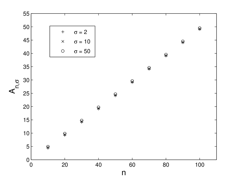
Figure 1: Solution of Eq. (62), for different values of $\sigma$ and $n$

For all the values of $\sigma$ investigated, $A_{n,\sigma}\simeq\frac{n}{2}$. The large $n$ behaviour of $A_{n,\sigma}$ is investigated in C. The entropy, in the $U$ representation is:

$$S(U,V)=\frac{n}{3}\log V+\log Y_{n,\sigma}(U)+\log{c_{n}\sqrt{\frac{\pi\sigma}{2}}e^{\frac{\sigma}{2}}}$$ (63)

where

$$Y_{n,\sigma}(U)=U^{\frac{n}{2}}\int_{0}^{\infty}dxx^{\frac{n}{2}-1}\left(1+\texttt{erf}\left[\frac{A_{n,\sigma}(1-x)-\sigma}{\sqrt{2\sigma}}\right]\right)$$ (64)

In agreement with Eq. (48), the dependence of the entropy on $U$ is of the type $\frac{n}{2}\log U$. The integral $Y_{n,\sigma}$ has been obtained by using the change of variable $x=e/U$, where $e$ denotes energy.

The Gaussian ensemble of Eq. (59) interpolates between canonical and microcanonical ensembles as does the Tsallis ensemble [11]. In fact, on one hand $f(x)\rightarrow e^{x}$ as $\sigma\rightarrow+\infty$, and, on the other $f(x)\rightarrow\sqrt{2\pi\sigma}\delta(x)$ as $\sigma\rightarrow 0$ (the vanishing term $\sqrt{2\pi\sigma}$ is not a problem because it will be cancelled with the normalization).

Further, based on the fact that the Gaussian ensemble of index $\sigma$ well describes the statistics of a large component of a large isolated system, we deduce that it must well approximate the Tsallis statistics of index $\alpha_{q}=\sigma$ in the case $n,\alpha_{q}\gg 1$. This fact is illustrated in Figure 2, where we have plotted the unnormalized Tsallis distribution $\left(1+\frac{n}{2\alpha_{q}}(1-\frac{e}{U})\right)^{\alpha_{q}-1}e^{\frac{n}{2}-1}$, for $\alpha_{q}=50,n=60,U=10$, and fitted it to the unnormalized gaussian statistics $\exp[A(1-e/U)-\frac{(A(1-e/U))^{2}}{2\sigma}]e^{\frac{n}{2}-1}$ with $U,\sigma,A$ as free parameters. The fit is very good ($1-R^{2}=O(10^{-4})$) and the fitting parameter matched quite well the expected values: $\sigma=48.36\simeq\alpha_{q}=50$, $U=10$, $A=29.51\simeq A_{n=60,\sigma=50}=29.63$.

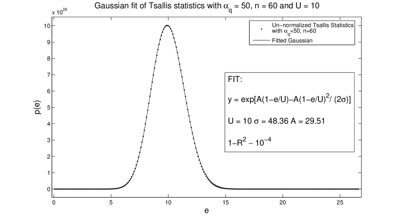
Figure 2: Gaussian fit of Tsallis statistics for $\alpha_{q}=50,n=60,U=10$. The dual Gaussian ensemble approximates Tsallis ensembles for large values of $n$ and $\alpha_{q}$

5.3 Fermi-like ensemble

The theory developed so far allows us to construct mechanical models of thermodynamics with the most diverse types of distributions. For example one may ask whether it would be possible to have an ensemble with a Fermi-like distribution. This is possible for the ideal gas case. We will describe this ensemble as an illustration of the theory, without discussing whether it really applies to some many-particle physical system. The Fermi-like statistics uses the choice:

$$F(x) = \log(e^{x}+1)$$ (65)

$$f(x) = \frac{1}{e^{-x}+1}$$ (66)

with no finite cut-off. The solutions $A_{n}$ of the energy constraint equation (45):

$$I(A,n)=\int_{0}^{\infty}dy\frac{y^{\frac{n}{2}-1}(A-y)}{e^{y-A}+1}=0$$ (67)

have been evaluated numerically and shown in Fig. 3 for the values $n=10,20,...,100$. From the figure we see that, $A_{n}\simeq n$. This fact is analyzed in more details in D

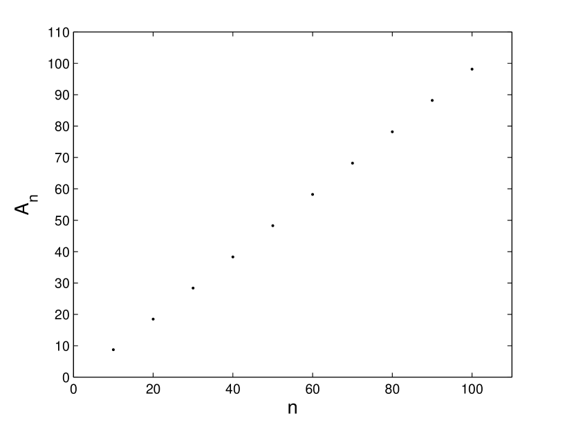
Figure 3: Solution of Eq. (67) for different values of $n$.

Adopting the $(U,V)$ parametrization, the ensemble, is:

$$\rho(\mathbf{z};U,V)=\frac{\left[e^{-A_{n}(1-\frac{H(\mathbf{z};V)}{U})}+1\right]^{-1}}{\int d\mathbf{z}\left[e^{-A_{n}(1-\frac{H(\mathbf{z};V)}{U})}+1\right]^{-1}}$$ (68)

or, alternatively:

$$\rho(\mathbf{z};\beta,V)=\frac{\left[e^{-A_{n}+\beta H(\mathbf{z};V)}+1\right]^{-1}}{\int d\mathbf{z}\left[e^{-A_{n}+\beta H(\mathbf{z};V)}+1\right]^{-1}}$$ (69)

if the $(\beta,V)$ parametrization is adopted. Using Eq. (26) gives the entropy. Adopting the $(U,V)$ parametrization, this is given by

$$S(U,V)=\log{c_{n}}+\frac{n}{3}\log{V}+\log{J_{n}(U)}$$ (70)

where

$$J_{n}(U)=U^{\frac{n}{2}}\int_{0}^{\infty}dxx^{\frac{n}{2}-1}\log\left(e^{A_{n}(1-x)}+1\right)$$ (71)

In agreement with Eq. (48), the dependence of the entropy on $U$ is of the type $\frac{n}{2}\log U$. The integral $J_{n}$ has been obtained by using the change of variable $x=e/U$, where $e$ denotes energy.

6 Discussion and conclusion

In this work we addressed some fundamental issues raised recently in statistical mechanics, namely whether a theoretical basis can be provided for non-standard (i.e. neither canonical nor microcanonical) ensembles, which are often encountered in the most diverse fields of physics. Following a line initiated in Refs. [2, 3], we used Boltzmann’s original approach based on the “heat theorem”, in order to provide a fresh look on the subject. By generalizing the duality property observed in the Tsallis case, we have been able to define the class of dual statistics, which includes the Tsallis ensembles as particular cases. The generalization scheme is represented in Fig. 4.

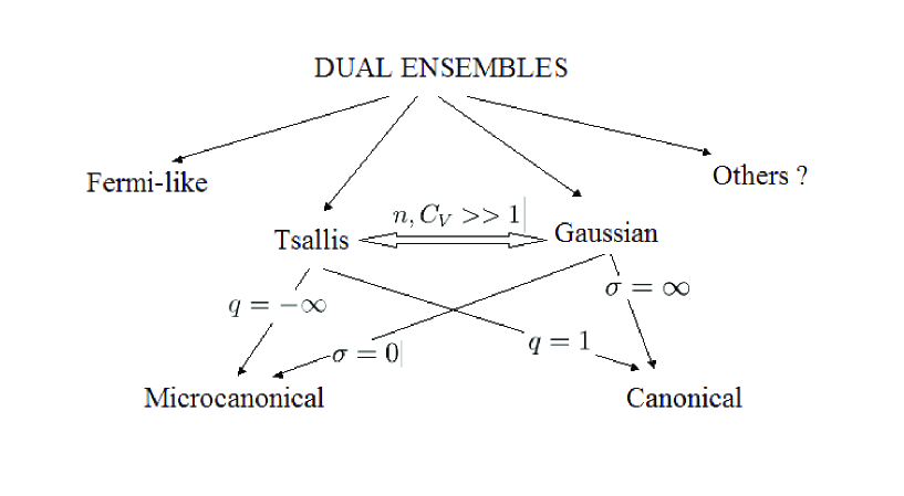
Figure 4: Generalization scheme. Tsallis ensembles, Gaussian ensembles, Fermi-like ensemble, and possibly other kinds of ensembles belong to the class of dual orthodes. Canonical and microcanonical are special instances of Tsallis and Gaussian ensembles. For large systems ($n>>1$) Gaussian and Tsallis ensemble coincide if $\sigma=\frac{1}{1-q}=C_{V}>>1$.

Thanks to the proposed generalization it is possible to provide a theoretical basis for many non-standard statistics other than Tsallis’, such as the gaussian and the Fermi-like statistics. For all such non-standard orthodes the heat theorem holds, namely the usual thermodynamic relations are recovered. In this paper we also have provided a general formula for the entropy associated to any dual orthode. This allowed us to write down the expression of entropy for the Gaussian ensemble, which has never been done before. To use the same expression as Gallavotti [4], all dual orthodes provide “mechanical models of thermodynamics”. This result is not trivial since the only known orthodes were the microcanonical ensemble, the canonical ensemble and its variants like the grand canonical ensemble and the pressure ensemble [4]. Despite the fact that the class of orthodes is quite vast, the microcanonical and the canonical ensembles still play a special role in statistical mechanics because they are cases of “hidden dual statistics”. They do not rely on the employment of the energy constraint, which constitutes the mechanism through which it is possible to construct non-standard dual orthodes.

One interesting result is that the classical ideal gas thermodynamics follows from any dual ensemble, thus revealing that this occurrence is not special for the standard statistics. This fact was already noticed for the Tsallis case a few years ago [10], although its orthodicity was not yet clearly recognized. It also suggests that there is a one-to-one correspondence of states obtained in different dual ensembles, i.e. there is an equivalence of all dual ensembles. Such equivalence holds no matter the number of degrees of freedom, and, of course, may break as one considers more realistic Hamiltonian models of systems with phase transitions. We also like to stress that all dual orthodes are equivalent also in another sense, namely the sense first investigated by Gibbs [12] for the canonical and microcanonical ensembles. In the thermodynamic limit ($n\rightarrow\infty$) and for the free gas model, the canonical ensemble is so peaked around the average energy value that it is practically undistinguishable from the microcanonical one [13]. The same kind of equivalence occurs for any dual statistics provided that $A_{n}\rightarrow\infty$ in the thermodynamic limit, which is indeed the case observed in the examples considered in this paper. This is because the distribution is expressed in terms of the quantity $f\left(A_{n}\frac{U-e}{U}\right)$ which tends to the Dirac delta (times an unimportant proportionality factor), centered around $U$:

$$f\left(A_{n}\frac{U-H}{U}\right)\rightarrow const\times\delta(U-H)$$ (72)

This follows from the asymptotic formula $h(kx)\rightarrow\frac{\int dyh(y)}{k}\delta(x)$, as $k\rightarrow\infty$.

Appendix A Proof of the Generalized Equipartition Theorem of Eq. (32)

Let us calculate explicitly the average value of $p_{i}\frac{\partial H}{\partial p_{i}}$. Regardless of the parametrization one has:

$$\left\langle p_{i}\frac{\partial H}{\partial p_{i}}\right\rangle_{\rho} = \frac{1}{G}\int d\textbf{z}p_{i}\frac{\partial H}{\partial p_{i}}f[\beta(U-H)]$$

$$= -\frac{1}{\beta G}\int d\textbf{z}p_{i}\frac{\partial}{\partial p_{i}}F[\beta(U-H)]$$

$$= -\frac{1}{\beta G}\left[\left[p_{i}F[\beta(U-H(\textbf{z};V))]\right]_{\textbf{z}\in\partial\mathcal{D}}-\int d\textbf{z}F[\beta(U-H)]\right]$$

Where we integrated by parts over $p_{i}$ to obtain the third line. From Eq.s (27) and (28) follows:

$$\left\langle p_{i}\frac{\partial H}{\partial p_{i}}\right\rangle_{\rho}=\frac{1}{\beta}\frac{\mathcal{G}}{G}$$ (74)

According to the parametrization adopted this would be either Eq. (30) or (31).

Appendix B Proof of orthodicity in the $\beta,V$ parametrization

In the $\beta,V$ parametrization $U$ is a function of $(\beta,V)$. Therefore $F$ is a function of $(\mathbf{z};U,V)$, and $\mathcal{G}$ (Eq. 27) and $S_{\rho}$ (Eq. 26) are functions of $(\beta,V)$. Let us calculate the partial derivatives of $S$

$$\frac{\partial S_{\rho}}{\partial\beta} = \frac{1}{\mathcal{G}}\frac{\partial}{\partial\beta}\int d\textbf{z}F(\beta(U-H))$$ (75)

$$= \frac{1}{\mathcal{G}}\int d\textbf{z}f(\beta(U-H))\left[(U-H)+\beta\frac{\partial U}{\partial\beta}\right]$$

$$= -\frac{G}{\mathcal{G}}\langle H-U\rangle_{\rho}+\frac{G}{\mathcal{G}}\beta\frac{\partial U}{\partial\beta}=\frac{1}{T_{\rho}}\frac{\partial U_{\rho}}{\partial\beta}$$

where we used the equation $U_{\rho}=<H>_{\rho}$ from the state definition (29) and the generalized equipartition theorem of Eq. (32).

$$\frac{\partial S_{\rho}}{\partial V_{\rho}} = \frac{1}{\mathcal{G}}\frac{\partial}{\partial V}\int d\textbf{z}F(\beta(U-H))$$ (76)

$$= \frac{1}{\mathcal{G}}\int d\textbf{z}f(\beta(U-H))\left[\beta\frac{\partial U}{\partial V}-\beta\frac{\partial H}{\partial V}\right]$$

$$= \beta\frac{G}{\mathcal{G}}\frac{\partial U}{\partial V}-\frac{G}{\mathcal{G}}\beta\left\langle\frac{\partial H}{\partial V}\right\rangle_{\rho}$$

$$= \frac{1}{T_{\rho}}\frac{\partial U_{\rho}}{\partial V_{\rho}}+\frac{P_{\rho}}{T_{\rho}}$$

where we used the expression for $P_{\rho}$ from Eq. (29) and the generalized equipartition theorem of Eq. (32). Combining all together:

$$dS=\frac{\frac{\partial U_{\rho}}{\partial\beta}d\beta+\frac{\partial U_{\rho}}{\partial V_{\rho}}dV_{\rho}+P_{\rho}dV_{\rho}}{T_{\rho}}=\frac{dU_{\rho}+P_{\rho}dV_{\rho}}{T_{\rho}}$$ (77)

Appendix C Large $n$ behaviour of the coefficients $A_{n,\sigma}$

Eq. (62) can be recast in the following form:

$$\int_{0}^{\infty}dyg_{n}(y)e^{-\frac{(A-y)^{2}}{2\sigma}}=A\int_{0}^{\infty}dyg_{n}(y)y^{-1}e^{-\frac{(A-y)^{2}}{2\sigma}}$$ (78)

where

$$g_{n}(y)\doteq\frac{y^{\frac{n}{2}}e^{-y}}{\int_{0}^{\infty}y^{\frac{n}{2}}e^{-y}}\theta(y)$$ (79)

and $\theta$ is Heaviside’s step function. Its Fourier transform is:

$$\hat{g}_{n}(k)=(1-ik)^{-\frac{n}{2}-1}$$ (80)

Using the formula $\lim_{N\rightarrow\infty}\left(1+\frac{x}{N}\right)^{N}=e^{x}$, we have:

$$\lim_{n\rightarrow\infty}\hat{g}_{n}(k)=e^{ik\left(\frac{n}{2}+1\right)}$$ (81)

therefore:

$$\lim_{n\rightarrow\infty}g_{n}(y)=\delta\left(y-\left(\frac{n}{2}+1\right)\right).$$ (82)

Using this result Eq. (78), becomes, for very large $n$:

$$A\simeq\frac{n}{2}$$ (83)

This result does not depend on $\sigma$.

Appendix D Large $n$ behaviour of the coefficients $A_{n}$ for the Fermi-like case

Figure 3 suggests that, in the limit $n\rightarrow\infty$, $A_{n}\simeq n$. In this appendix section we provide a simple consistency argument to support the claim that $A_{n}\simeq n$. Let us assume that for very large $n$, $A_{n}\simeq n$. Then we should have from Eq. (67):

$$\int_{0}^{\infty}dy\frac{y^{\frac{n}{2}}}{e^{y-n}+1}\simeq n\int_{0}^{\infty}dy\frac{y^{\frac{n}{2}-1}}{e^{y-n}+1}$$ (84)

Equating the first derivative of the integrand in the left hand side to zero, gives:

$$y=\frac{n}{2}(1+e^{n-y})$$

which is satisfied for $y=n$. This means that an extremum (a maximum as we will see) is attained for $y=n$. The value taken by the integrand at the maximum is $\frac{n^{\frac{n}{2}}}{2}$ which increases very quickly. The second derivative, calculated at $y=n$, is:

$$\frac{1}{4}\left[\left(\frac{n}{2}-1\right)n^{-\frac{n}{2}+1}-n^{\frac{n}{2}}\right]$$ (85)

which tends to $-\infty$ very quickly. This indicates that the integrand becomes very sharply peaked around $y=n$ as $n$ increases. Therefore, as an approximation, we can replace $y$ with $n$, and see that $y^{\frac{n}{2}}\simeq ny^{\frac{n}{2}-1}$, thus getting Eq. (84).

References

References

- [1] C. Tsallis. Possible generalization of Boltzmann-Gibbs statistics. Journal of statistical physics, 52:479, 1988.
- [2] Michele Campisi and Gokhan B. Bagci. Tsallis ensemble as an exact orthode. Physics Letters A, 362(1):11–15, February 2007.
- [3] Michele Campisi. On the limiting cases of nonextensive thermostatistics. Physics Letters A, to appear, 2007. arXiv:cond-mat/0611068.
- [4] G. Gallavotti. Statistical mechanics. A short treatise. Springer Verlag, Berlin, 1995.
- [5] Ludwig Boltzmann. Über die Eigenschaften monocyklischer und anderer damit verwandter Systeme. Crelle’s Journal, 98:68–94, 1884. Reprinted in Hasenöhrl (ed.), Wissenschaftliche Abhandlungen, vol. 3, pp. 122-152. New York: Chelsea.
- [6] M. Campisi. On the mechanical foundations of thermodynamics: The generalized Helmholtz theorem. Stud. Hist. Philos. M. P., 36:275–290, 2005.
- [7] A.I. Khinchin. Mathematical foundations of statistical mechanics. Dover, New York, 1949.
- [8] S. Martínez, F. Pennini, A. Plastino, and C. Tessone. On the equipartition and virial theorems. Physica A, 305, 2002.
- [9] M. P. Almeida. Generalized entropy from first principles. Physica A, 300:424–432, 2001.
- [10] S. Abe, S. Martinez, F. Pennini, and A. Plastino. Nonextensive thermodynamic relations. Phys. Lett. A, 281:126, 2001.
- [11] Murty S. S.Challa and J. H.Hetherington. Gaussian ensemble as an interpolating ensemble. Physical Review Letters, 60(2):77–80, 1988.
- [12] J.W. Gibbs. Elementary principles in statistical mechanics. Yale University Press, Yale, 1902. reprinted by Dover, New York, 1960.
- [13] K. Huang. Statistical mechanics. John Wiley & Sons, Singapore, 2nd edition, 1963.