A reduced model for shock and detonation waves. II. The reactive case.

Abstract

We present a mesoscopic model for reactive shock waves, which extends the model proposed in [9]. A complex molecule (or a group of molecules) is replaced by a single mesoparticle, evolving according to some Dissipative Particle Dynamics. Chemical reactions can be handled in a mean way by considering an additional variable per particle describing the progress of the reaction. The evolution of the progress variable is governed by the kinetics of a reversible exothermic reaction. Numerical results give profiles in qualitative agreement with all-atom studies.

1 Introduction

Whereas multimillion atoms simulations are nowadays common in molecular dynamics studies with simple potentials, the time and space scales numerically tractable are still far from being macroscopic. The situation is even worse for nonequilibrium processes such as shock and detonation waves. Indeed, the simulation of detonation requires the description of a thin shock front, moving at high velocity, usually using a complicated empirical potential able to treat chemical events happening (dissociation, recombination - see [1] for a fundamental reference). To this end, toy molecular models were proposed at the early stages of molecular simulations of detonation (see e.g. [2]), until the first all-atom studies in the nineties [3, 4], allowed by the development of bond order potentials. Nevertheless, despite recent advances in the development of reactive force fields [5], the simulation of the decomposition of real materials still remains confined to small systems sizes and short time scales (see for example [6] for a state of the art study). A direct simulation of the macroscopic reaction zone of a real material is well beyond current computer capabilities, highlighting the importance of the development of reduced model for detonation.

Following the pioneering works of Holian and Strachan [7, 8], a reduced model for (inert) shock waves was proposed in [9], where complex molecules are replaced by mesoparticles. These mesoparticles are described by their positions, momenta, and have an additional degree of freedom: their internal energies. This model is strongly inspired by Dissipative Particle Dynamics (DPD) [10] with conserved energy [11, 12]. In reduced models for shock waves [8, 9], one mesoparticle stands for one complex molecule. Reduced models are interesting in practice to simulate large systems, and as an intermediate step in a truly multiscale approach, where some parts of the system could be treated with all-atom models, while the remaining parts would be treated with hydrodynamic models, implemented with particle discretizations such as Smoothed Particle Hydrodynamics [13, 14]. A first step to such a general formalism in the equilibrium case is proposed in [15].

In the reactive case, exothermic chemical reactions are triggered when the shock passes, and the energy liberated sustains the shock. To model detonation at the mesoscopic level, we introduce a new variable per mesoparticle, namely a progress variable, which characterizes the progress of the chemical decomposition. The dynamics can then be split into three elementary physical processes:

1. the translational dynamics of the particles, given by the dynamics of inert materials [9];

2. the evolution of chemical reactions through some kinetics on the progress variable;

3. the exothermicity of the reaction: energy transfers between chemical and mechanical plus internal energies have to be precised.

The paper is organized as follows. After summarizing the dynamics for inert materials, we turn to the evolution of the progress variable and the treatment of the exothermicity in the reactive case. A numerical implementation relying on some splitting based on the decomposition of the dynamics into elementary physical processes is also proposed. Numerical results eventually confirm the correct behavior of the model. Let us emphasize that we aim here at proposing a dynamics in qualitative agreement with all-atom detonation simulations, giving correct orders of magnitude for the speed of the detonation front and the width of the reaction zone. This dynamics is of course parametrized by a certain collection of parameters describing the initial and the final material, as well as the chemical kinetics. We however tried to limit their total number to keep only the essential ones, and give some tracks to estimate these parameters from small all-atom numerical simulations or physical experiments.

2 A reduced model for inert shock waves

We briefly recall here the inert model presented in [9]. We consider a system of $N$ mesoscopic particles with positions $(q_{1},\dots,q_{N})$, momenta $(p_{1},\dots,p_{N})$, masses $(m_{1},\dots,m_{N})$, and internal energies $(\epsilon_{1},\dots,\epsilon_{N})$. The internal temperature $T_{i}$ is defined as $T_{i}^{-1}=\frac{ds(\epsilon_{i})}{d\epsilon_{i}}$. The function $s\equiv s(\epsilon)$ is the microscopic equation of state of the system, and relates the microscopic entropy $s$ (arising from the existence of degrees of freedom not explicitely represented) and the internal energy $\epsilon$. As a first approximation, $s(\epsilon)=C_{v}\ln\epsilon$. Denoting by $\bar{T}$ the reference temperature, $\beta=1/(k_{\rm B}\bar{T})$, and $V$ the interaction potential, the system evolves in the inert case as

$$dq_{i} = \frac{p_{i}}{m_{i}}\,dt,$$

$$dp_{i} = \sum_{j,\,j\not=i}-\nabla_{q_{i}}V(r_{ij})\,dt-\gamma_{ij}\chi^{2}(r_{ij})v_{ij}\,dt$$ (1)

$$\quad+\sigma\chi(r_{ij})dW_{ij},$$

$$d\epsilon_{i} = \frac{1}{2}\sum_{j,\,j\not=i}\chi^{2}(r_{ij})\left(\gamma_{ij}v_{ij}^{2}-\frac{d\sigma^{2}}{2}\left(\frac{1}{m_{i}}+\frac{1}{m_{j}}\right)\right)dt-\sigma\,\chi(r_{ij})v_{ij}\cdot dW_{ij},$$

where $r_{ij}=|q_{i}-q_{j}|$, $v_{ij}=\frac{p_{i}}{m_{i}}-\frac{p_{j}}{m_{j}}$, $\chi$ is a weighting function (with support in $[0,r_{\rm c}]$ for some cut-off radius $r_{\rm c}$), and the processes $W_{ij}$ are independent $d$-dimensionnal standard Wiener processes such that $W_{ij}=-W_{ji}$. The fluctuation-dissipation relation relating the frictions $\gamma_{ij}$ and the magnitude $\sigma$ of the random forcing is

$$\gamma_{ij}=\sigma^{2}\beta_{ij}/2,\quad\beta_{ij}=\frac{1}{k_{\rm B}T_{ij}}=\frac{1}{2k_{\rm B}}\left(\frac{1}{T_{i}}+\frac{1}{T_{j}}\right).$$ (2)

Notice that we implicitely defined the temperature $T_{ij}$ as the average internal temperature: $T_{ij}=(T_{i}+T_{j})/2$. It can be shown that the measure

$$d\rho(q,p,\epsilon)=Z^{-1}{\rm e}^{-\beta H(q,p)}\exp\left(\sum_{i}\frac{s(\epsilon_{i})}{k_{\rm B}}-\beta\epsilon_{i}\right)\delta_{E=E_{0}}\,\delta_{P=P_{0}}\,\,dq\,dp\,d\epsilon$$

is an invariant measure of the dynamics. In practice, we set $\sigma^{2}=2\gamma/\beta$ and therefore $\gamma_{ij}/\gamma=\bar{T}/T_{ij}$. The parameters used in the inert dynamics can be estimated as in [9].

3 Evolution of the progress variable

In the reactive case, chemical reactions are triggered when the shock passes. To model the progress of the reaction, an additional degree of freedom, a progress variable $\lambda_{i}$, is attached to each particle. For the model reaction

$$2\text{AB}\rightleftarrows\text{A}_{2}+\text{B}_{2},$$ (3)

the state $\lambda=0$ corresponds to a molecule AB, whereas the state $\lambda=1$ corresponds to A₂ + B₂. Representing the progress of the chemical reaction by a real-value parameter seems questionable when a mesoparticle stands for a single molecule. The progress variable should therefore rather be seen as some dissociation probability, or progress along some free energy profile.

Since the model reaction (3) involves two species on each side, we postulate for example the reversible evolution:

$$\frac{d\lambda_{i}}{dt} = \sum_{j\not=i}\omega_{r}(r_{ij})\left[K_{1}(T_{ij})(1-\lambda_{i})(1-\lambda_{j})+K_{2}(T_{ij})\lambda_{i}\lambda_{j}\right]$$ (4)

when $0\leq\lambda_{i}\leq 1$, and $\frac{d\lambda_{i}}{dt}=0$ otherwise (in order to ensure that the progress variables remains in $[0,1]$). The function $\omega_{r}$ in (4) is a weight function (with support in $[0,r_{\rm reac}]$), and the mean temperature $T_{ij}$ is defined as in (2). We term this reaction ’reversible’ since $\lambda_{i}$ can either increase or decrease. The motivation for the postulated kinetics (4) is the physical picture of a second-order reaction, where two molecules have to interact for the dissociation process to occur. Of course, many other kinetics are also possible, such as the first-order irreversible evolution

$$\frac{d\lambda_{i}}{dt}=K(\langle T_{i}\rangle)(1-\langle\lambda_{i}\rangle),$$

where $\langle h\rangle=\sum_{j}\omega_{r}(r_{ij})h_{i}$ denotes a local spatial average. The choice of the reaction kinetics is really a modelling choice, depending on the physical context.

The reaction constants $K_{1}$, $K_{2}$ are assumed to depend only on internal temperatures of particles. For example, a possible form in the Arrhénius spirit is:

$$K_{1}(T)=Z_{1}\ {\rm e}^{-E_{1}/k_{\rm B}T},\qquad K_{2}(T)=Z_{2}\ {\rm e}^{-E_{2}/k_{\rm B}T}.$$ (5)

In this expression, $E_{1}$ and $E_{2}$ are the activation energies of, respectively, the forward and backward reactions. In view of our choice (4) of reaction kinetics, the total increment of the progress variable is therefore the sum of all elementary pair increments, which is very much in the DPD spirit. The parameters $Z_{1},Z_{2},E_{1},E_{2}$ in the above equation can be obtained from all-atom decomposition simulations or directly from experiments. In particular, $Z_{1}$ and $E_{1}$ can be extracted in the Arrhénius framework from the analysis of decomposition rates at different initial temperatures. The constants $Z_{2}$ and $E_{2}$ can be evaluated using thermochemical data (formation enthalpies).

For very exothermic reactions, $E_{2}\gg E_{1}$, and both energies are large since the activation energy is usually large for energetic materials. The increment of a given reaction rate is therefore non-negligible only if the material is sufficiently heated. In practice, this can be achieved when a strong shock is initiated in the system. If this shock is not strong enough, chemical reactions do not occur fast enough, and since the energy release is not sufficient, the shock wave is weakened until it transforms into a sonic wave. On the contrary, if the shock wave is strong enough, chemical reactions happen close enough to the detonation front, and the energy released sustains the shock wave such that it transforms into a stationary detonation wave. The progress of the reaction also modifies the mechanical properties of the material. In particular, reaction products usually have a larger specific volume than reactants (at fixed thermodynamic conditions). Therefore, some expansion is expected. The changes in the nature of the molecules are taken into account by introducing two additional parameters $k_{a},k_{E}$ and using some mixing rule such as Berthelot’s rule. When the interaction potential is of Lennard-Jones form, the interaction between the mesoparticles $i$ and $j$ is then given by

$$V(r_{ij},\lambda_{i},\lambda_{j})=4E_{ij}\,\left(\left(\frac{a_{ij}}{r_{ij}}\right)^{12}-\left(\frac{a_{ij}}{r_{ij}}\right)^{6}\right),$$ (6)

with

$$E_{ij}=E\sqrt{(1+k_{E}\lambda_{i})(1+k_{E}\lambda_{j})},$$

and

$$a_{ij}=a\left(1+k_{a}\frac{\lambda_{i}+\lambda_{j}}{2}\right).$$

When the reaction is complete, the material initially described by a Lennard-Jones potential of parameters $a,E$ is then described by a Lennard-Jones of parameters $a^{\prime}=a(1+k_{a})$ and $E^{\prime}=E(1+k_{E})$.

4 Treatment of the exothermicity

We denote by $\Delta E_{\rm exthm}$ the exothermicity of the reaction (3). It is expected that $\Delta E_{\rm exthm}=E_{2}-E_{1}$. We assume that the energy is liberated progressively during the reaction, in a manner that the total energy of the system (chemical, mechanical, internal) is preserved:

$$dH_{\rm tot} = d\left[\sum_{i=1}^{N}\frac{p_{i}^{2}}{2m_{i}}+\epsilon_{i}+(1-\lambda_{i})\Delta E_{\rm exthm}+\sum_{1\leq i<j\leq N}V(r_{ij},\lambda_{i},\lambda_{j})\right]=0.$$

In order to propose a dynamics satisfying this condition, we have to make an additional assumption about the evolution of the system. Neglecting diffusive processes, we require that, during the elementary step corresponding to exothermicity, the total energy of a given mesoparticle does not change:

$$d\left[\frac{1}{2}\sum_{i\not=j}V(r_{ij},\lambda_{i},\lambda_{j})\right]+d\left(\frac{p_{i}^{2}}{2m_{i}}+\epsilon_{i}-\Delta E_{\rm exthm}\lambda_{i}\right)=0.$$ (7)

We then consider evolutions of momenta and internal energies balancing the variations in the total energy due to the variations of $\lambda$ (exothermicity, changes in potential energies). This is analogous to the fact that the variations of kinetic energy in (2) are compensated by variations of internal energies. It is expected that the chemical energy liberated by the reaction is converted into internal energy and kinetic energy. It therefore remains to precise the quantitative distribution of the energy. This is done using a predetermined ratio $0<c<1$. This ratio could be measured in gas phase decomposition experiments, using spectroscopy measurements (possibly numerical simulations as well, by computing the temperature of internal degrees of freedom after the reaction). Alternatively, it is possible to postulate that $c$ should be comparable to the ratio of the number of external degrees of freedom for the products of the dissociation of one complex molecule (denoted by $N_{\rm e}$), divided by the total number of degrees of freedom $N_{\rm t}$ in a complex molecule (assuming some equipartition of the liberated chemical energy). For exothermic chemical decompositions, it is expected that a single complex molecule breaks into several smaller molecules (still aggregated in a single mesoparticle), so that the above ratio $N_{\rm e}/N_{\rm t}$ should be close to 0.5. Let us however emphasize at this point that numerical profiles obtained here are robust enough with respect to the choice of $c$.

For the internal energies, the exothermicity of the reaction is modelled as $d\epsilon_{i}=d{\cal E}_{i}$ with

$$d{\cal E}_{i}=-c\left(d\left[\frac{1}{2}\sum_{i\not=j}V(r_{ij},\lambda_{i},\lambda_{j})\right]-\Delta E_{\rm exthm}d\lambda_{i}\right).$$

For the momenta, we consider process ${\cal P}_{i}$ with $dp_{i}=d{\cal P}_{i}$ such that

$$d\left(\frac{p^{2}_{i}}{2m}\right) = -(1-c)\left(d\left[\frac{1}{2}\sum_{i\not=j}V(r_{ij},\lambda_{i},\lambda_{j})\right]-\Delta E_{\rm exthm}d\lambda_{i}\right).$$

We explain in the next section how this is done in practice (see Eq. (5)).

Let us emphasize at this point that there are many other possible ways to treat the exothermicity. For instance, it would be possible to consider instantaneous reactions (jump processes for which $\lambda$ changes from 0 to 1) occuring at random times, the probability of reaction depending on the progress variable. However, it is not clear whether such a dynamics is reversible, since the reverse reaction requires particles to have large kinetic and internal energies. In comparison, the process described here is progressive and therefore, much more reversible.

Finally, we propose the following dynamics to describe reactive shock waves:

$$dq_{i} = \frac{p_{i}}{m_{i}}\,dt,$$

$$dp_{i} = \sum_{j,\,j\not=i}-\nabla_{q_{i}}V(r_{ij},\lambda_{i},\lambda_{j})\,dt-\gamma_{ij}\chi^{2}(r_{ij})v_{ij}\,dt+\sigma\chi(r_{ij})dW_{ij}+d{\cal P}_{i},$$ (8)

$$d\epsilon_{i} = \frac{1}{2}\sum_{j,\,j\not=i}\chi^{2}(r_{ij})\left(\gamma_{ij}v_{ij}^{2}-\frac{d\sigma^{2}}{2}\left(\frac{1}{m_{i}}+\frac{1}{m_{j}}\right)\right)\,dt-\sigma\,\chi(r_{ij})v_{ij}\cdot dW_{ij}+d{\cal E}_{i},$$

$$d\lambda_{i} = \sum_{j\not=i}\omega_{r}(r_{ij})\left[K_{1}(T_{ij})(1-\lambda_{i})(1-\lambda_{j})+K_{2}(T_{ij})\lambda_{i}\lambda_{j}\right]\,dt,$$

where $d{\cal P}_{i}$, $d{\cal E}_{i}$ are such that (7) holds, i.e. the total energy is conserved. The fluctuation-dissipation relation relating $\gamma_{ij}$ and $\sigma$ is still (2). Notice also that the inert dynamics (2) of [9] is recovered when $Z_{1}=Z_{2}=0$, starting from $\lambda_{i}=0$ for all $i$.

5 Numerical implementation

The numerical integration of (4) is done using a decomposition of the dynamics into elementary stochastic differential equations. We denote by $\phi^{t}_{\rm inert}$ the flow associated with the dynamics (2), and by $\phi^{t}_{\rm reac}$ the flow associated with the remaining part of the dynamics (4): $\forall 1\leq i\leq N$,

$$\left\{\begin{array}[]{cl}d\lambda_{i}=&\sum_{j\not=i}\omega_{r}(r_{ij})\left[K_{1}(T_{ij})(1-\lambda_{i})(1-\lambda_{j})+K_{2}(T_{ij})\lambda_{i}\lambda_{j}\right]\,dt,\\ dp_{i}=&d{\cal P}_{i},\\ d\epsilon_{i}=&d{\cal E}_{i}.\\ \end{array}\right.$$ (9)

A one-step integrator for a time-step $\Delta t$ is constructed as

$$(q^{n+1},p^{n+1},\epsilon^{n+1},\lambda^{n+1})=\Phi^{\Delta t}_{\rm reac}\circ\Phi^{\Delta t}_{\rm inert}(q^{n},p^{n},\epsilon^{n},\lambda^{n}).$$

A possible numerical flow $\Phi^{\Delta t}_{\rm inert}$ is given in [9].

Let us now construct a numerical flow $\Phi^{\Delta t}_{\rm reac}$ approximating the flow $\phi^{\Delta t}_{\rm reac}$. Denoting $(q^{n+1},\tilde{p}^{n},\tilde{\epsilon}^{n},\lambda^{n})=\Phi^{\Delta t}_{\rm inert}(q^{n},p^{n},\epsilon^{n},\lambda^{n})$, we first integrate the evolution equation on the progress variables $\lambda_{i}$ using a first-order explicit integration:

$$\tilde{\lambda}_{i}^{n+1} = \lambda_{i}^{n}+\sum_{j\not=i}\omega_{r}(r^{n+1}_{ij})\left[K_{1}(\tilde{T}^{n}_{ij})(1-\lambda^{n}_{i})(1-\lambda^{n}_{j})K_{2}(\tilde{T}^{n}_{ij})\lambda^{n}_{i}\lambda^{n}_{j}\right]\ \Delta t.$$

We then set $\lambda_{i}^{n+1}=\min(\max(0,\tilde{\lambda}_{i}^{n+1}),1)$ in order to ensure that the progress variable remains between 0 and 1. Once all progress variables are updated, the variation $\delta E_{i}^{n}$ in the total energy of particle $i$ due to the variations of $\{\lambda_{j}\}$ is computed as

$$\delta E_{i}^{n} = (\lambda_{i}^{n+1}-\lambda_{i}^{n})\Delta E_{\rm exthm}+\frac{1}{2}\sum_{j\not=i}\left(V(r^{n+1}_{ij},\lambda_{i}^{n+1},\lambda_{j}^{n+1})-V(r^{n+1}_{ij},\lambda_{i}^{n},\lambda_{j}^{n})\right).$$

The conservation of total energy is then ensured through variations of internal and kinetic energies. The internal energies are updated as $\epsilon_{i}^{n+1}=\tilde{\epsilon}_{i}^{n}+c\,\delta E_{i}^{n}$. The update of $p_{i}^{n+1}$ is done by adding to $p_{i}^{n}$ a vector with random direction, so that the final momentum is such that the kinetic energy is correct. More precisely, when the dimension of the physical space is $d=2$ for example, an angle $\theta_{i}^{n}$ is chosen at random in the interval $[0,2\pi]$, the angles $(\theta_{i}^{n})_{i,n}$ being independent and identically distributed random variables. The new momentum $p_{i}^{n+1}$ is then constructed such that

$$p_{i}^{n+1}=p_{i}^{n}+\alpha^{n}(\cos\theta_{i}^{n},\sin\theta_{i}^{n}),$$

$$\frac{(p_{i}^{n+1})^{2}}{2m_{i}}=\frac{(\tilde{p}_{i}^{n})^{2}}{2m_{i}}+(1-c)\,\delta E_{i}^{n}.$$ (10)

Solving this equation in $\alpha^{n}$ gives the desired result.

6 Numerical results

We present in this section numerical results obtained for the dynamics (4) of a two-dimensional fluid. A shock is initiated using a piston of velocity $u_{\rm p}$ during a time $t_{\rm p}$. The initial conditions for the positions $q_{i}$, momenta $p_{i}$ and internal energies $\epsilon_{i}$ are sampled as proposed in [9].

We consider the following parameters, inspired by the nitromethane example (in which case the molecule CH₃NO₂ would replaced by a mesoparticle in a space of 2 dimensions). The parameters can be classified in four main categories, depending on whether they describe the mechanical properties of the material, characterize the inert dynamics and the chemical kinetics, or are related to the exothermicity. We consider here a system with

• (Material parameters) a molar mass $m=80$ g/mol, described by a Lennard-Jones potential of parameter $E_{\rm LJ}=3\times 10^{-21}$ J (melting temperature around 220 K) and $a=5$ Å, with a cut-off radius $r_{\rm cut}=15$ Å for the computation of forces. The changes in the parameters of the Lennard-Jones material during the reaction follow (6), using $k_{E}=0$ and $k_{a}=0.2$ (pure expansion).

• (Parameters of the inert dynamics) The microscopic state law is $\epsilon=C_{v}T$ with $C_{v}=10$ $k_{\rm B}$ (i.e., 20 degrees of freedom are not represented). The friction is $\gamma=10^{-15}$ kg/s, and the dissipation weighting function $\chi(r)=(1-r/r_{\rm c})$, with $r_{\rm c}=r_{\rm cut}$.

• (Chemical kinetics) For the chemical reaction (4), reaction constants are computed using (5) with $Z_{1}=Z_{2}=10^{17}$ s^-1, $E_{1}/k_{\rm B}=15000$ K, the exothermicity being $\Delta E_{\rm exthm}=6.25$ eV. The reaction weighting function $\omega(r)=\chi(r)$;

• (Exothermicity) we choose $c=0.5$.

The initial density of the system is $\rho=1.06$ g/cm^-3, and the initial temperature $\bar{T}=300$ K. The time-step used is $\Delta t=2\times 10^{-15}$ s. Figure 1 presents velocity profiles averaged in thin slices of the material in the direction of the shock, for a compression time $t_{\rm p}=2$ ps at a velocity $u_{\rm p}=5000$ m/s. We tested the independence of velocity profiles in the reaction zone with respect to different initial loadings $(t_{\rm p},u_{\rm p})=(1~{}{\rm ps},6000~{}{\rm m/s})$, $(t_{\rm p},u_{\rm p})=(2~{}{\rm ps},6000~{}{\rm m/s})$, $(t_{\rm p},u_{\rm p})=(3~{}{\rm ps},6000~{}{\rm m/s})$ and $(t_{\rm p},u_{\rm p})=(3~{}{\rm ps},5000~{}{\rm m/s})$.

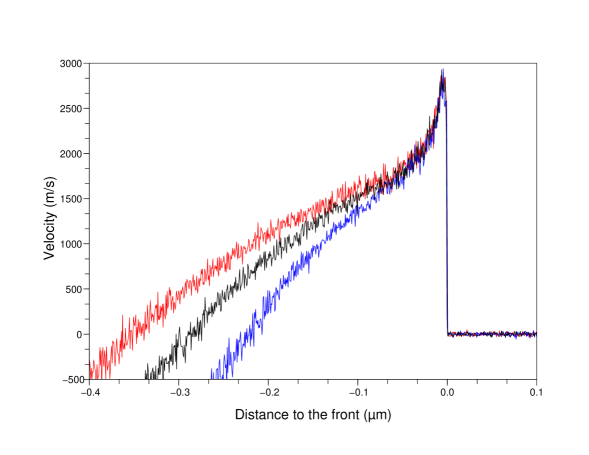
Figure 1: (color online) Velocity profiles in the material at different times, with shock fronts aligned (Black: $t=1.6\times 10^{-10}$ s; Blue: $t=2.0\times 10^{-10}$ s; Red: $t=2.4\times 10^{-10}$ s).

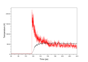
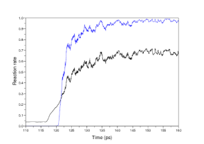
Figure 2: (color online) Left : variations of internal (red) and kinetic (black) temperatures in the direction of the shock, as a function of time in a slice of material. Right: evolution of the progress variable averaged in a slice of material as a function of time (blue). For comparison, a rescaled internal temperature profile is also presented (black).

The velocity of the shock front is constant, and approximately equal to $u_{\rm s}=1820$ m/s. Notice that the wave can be divided into three regions: the upstream region is unperturbed; the region around the shock front where chemical reactions happen is of constant width (approximately 300-400 Å, which is consistent with all-atoms studies, see for instance [16]); the downstream region is an autosimilar rarefaction wave. This profile is therefore reminiscent of ZND profiles [1] encountered in hydrodynamic simulations of detonation waves.

Figure 2 presents the evolution of internal and kinetic temperatures averaged in a slice of material in the direction of the shock as a function of time (Left), as well as the evolution of the average progress variables (Right). In particular, the reaction does not start immedialely at the shock front: the ignition asks first for a sufficient heating of the material (through an increasing internal energy), since the reaction constant are too low at temperatures lower than a few thousands Kelvins with the values chosen here.

7 Conclusion and perspectives

In conclusion, we extended the mesoscopic inert model for shock waves of [9] to the reactive case. The key idea is to introduce an additional variable describing the progress of the reaction, and to postulate an activated exothermic chemical reaction. Provided the initial loading is strong enough, the energy released by chemical reactions sustains the shock wave, whose front then travels unperturbed in the material, followed by a rarefaction wave.

Now that while the qualitative behavior of the model is granted, more quantitative studies must be pursued, where a careful comparison between all-atom numerical results and the profiles predicted by the reduced model proposed here are to be compared. Such studies were already performed in the inert case [8, 9].

A promising track for a real multiscale modelling of detonation waves would now be to further reduce the model proposed here, in order to obtain a description of matter at a scale truly intermediate between SPH and all-atom models. In such a model, random fluctuations would still be present, though of much lower magnitude; on the other hand, local thermodynamic fields (such as pressure) should also be introduced. Such an intermediate model is necessary to describe mesoscopic effects having an impact on the macroscopic features of the detonation, such as hot spot ignition.

References

- [1] W. Fickett and W.C. Davis, Detonation - Theory and Experiment (Dover Publications, 2000)
- [2] M. Peyrard, S. Odiot and E. Lavenir J.M. Schnur, J. Appl. Phys., 57 (1985) 2626
- [3] D.W. Brenner, D.H Robertson, M.L. Elert and C.T. White, Phys. Rev. Lett., 70(14) (1993) 2174
- [4] D.W. Brenner, D.H Robertson, M.L. Elert and C.T. White, Phys. Rev. Lett., 76(12) (1996) 2202
- [5] K.D. Nielson, A.C.T. Van Duin, J. Oxgaard, W.-Q. Deng and W.A. Goddard III, J. Phys. Chem. A, 109 (2005) 493
- [6] A. Strachan, A.C.T. van Duin, D. Chakraborty, S. Dasgupta and W.A. Goddard III, Phys. Rev. Lett., 91 (2003) 098301
- [7] B.L. Holian, Europhys. Lett., 64(3) (2003) 330
- [8] A. Strachan and B.L. Holian, Phys. Rev. Lett., 94(1) (2005) 014301
- [9] G. Stoltz, Europhys. Lett., 76(5) (2006) 849
- [10] P.J. Hoogerbrugge and J.M.V.A. Koelman, Europhys. Lett., 19(3) (1992) 155
- [11] J.B. Avalos and A.D. Mackie, Europhys. Lett., 40 (1997) 141
- [12] P. Español, Europhys. Lett., 40 (1997) 631
- [13] L.B. Lucy, Astron. J., 82(12) (1977) 1013
- [14] J.J. Monaghan, Annu. Rev. Astron. Astrophys., 30 (1992) 543
- [15] P. Español and M. Revenga, Phys. Rev. E, 67 (2003) 026705
- [16] A.J. Heim, N. Grønbech-Jensen, T.C. Germann, E.M. Kober, B.L. Holian and P.S. Lomdahl, Arxiv preprint, cond-mat/0601106 (2006)