Quasi-elastic solutions to the nonlinear Boltzmann equation for dissipative gases

Abstract

The solutions of the one-dimensional homogeneous nonlinear Boltzmann equation are studied in the QE-limit (Quasi-Elastic; infinitesimal dissipation) by a combination of analytical and numerical techniques. Their behavior at large velocities differs qualitatively from that for higher dimensional systems. In our generic model, a dissipative fluid is maintained in a non-equilibrium steady state by a stochastic or deterministic driving force. The velocity distribution for stochastic driving is regular and for infinitesimal dissipation, has a stretched exponential tail, with an unusual stretching exponent $b_{QE}=2b$, twice as large as the standard one for the corresponding $d$-dimensional system at finite dissipation. For deterministic driving the behavior is more subtle and displays singularities, such as multi-peaked velocity distribution functions. We classify the corresponding velocity distributions according to the nature and scaling behavior of such singularities.

I Introduction

I.1 Background and outline

The model of inelastic hard spheres is one of the most simple frameworks to describe granular gases (see e.g. Gold ; PoschelBrill ; usJPCM for reviews and further references). The contraction of phase space due to dissipative collisions leads to a non-equilibrium behavior that is markedly different from that of equilibrium systems (non-Gaussian velocity distributions, counter-intuitive hydrodynamics, breakdown of kinetic energy equipartition etc Gold ; PoschelBrill ; usJPCM ). In this paper, we study in detail the limit of quasi-elasticity Mcnamara2 ; Caglioti ; Benedetto ; Ramirez with particular emphasis on one-dimensional systems, that have already been the subject of some interest Mcnamara1 ; Sela ; bennaim ; Rosas .

The kinetic description is provided by the nonlinear Boltzmann equation. As we are interested in the velocity statistics of dissipative gases, we will restrict ourselves to homogeneous and isotropic solutions. Any spatial dependence will therefore be discarded. The time evolution of the velocity distribution function $F(v,t)$ is then governed by the following equationEB-Rap02 ; ETB ,

$$\partial_{t}F(v)+{\cal F}F\,=\,I(v|F)\equiv\int_{\bf n}\int d{\bf w}\,g^{\nu}\left[\frac{1}{\alpha_{0}^{\nu+1}}F(v^{**})F(w^{**})-F(v)F(w)\right].$$ (1)

Here ${\cal F}F$ represents the action of a driving mechanism, that injects energy into the system, and counterbalances the energy dissipated by inelastic collisions. Consequently, the system is expected to reach a non-equilibrium steady-state. In the equation above ${{\bf g}}={\bf v}-{\bf w}$ denotes the relative velocity of colliding particles with $g=|{\bf g}|$, $\int_{\bf n}(\cdots)=(1/\Omega_{d})\int d{\bf n}(\cdots)$ is an angular average over the surface area $\Omega_{d}=2\pi^{d/2}/\Gamma(\textstyle{\frac{1}{2}}d)$ of a $d$-dimensional unit sphere, and $g^{\nu}$ models the collision frequency. Note that in one dimension the integral $\int_{\bf n}$ is absent. We have absorbed constant factors in the time scale. Here $({\bf v}^{**},{\bf w}^{**})$ denote the restituting velocities that yield (${\bf v},{\bf w}$) as post-collisional velocities, i.e.

$${\bf v}^{**}\,=\,{\bf v}-\textstyle{\frac{1}{2}}(1+\alpha_{0}^{-1})({\bf g}\cdot{\bf n}){\bf n}\quad;\quad{\bf w}^{**}={\bf w}+\textstyle{\frac{1}{2}}(1+\alpha_{0}^{-1})({\bf g}\cdot{\bf n}){\bf n},$$ (2)

where (unit) vector ${\bf n}$ is parallel to the line of centers of the colliding particles. Note that ${\bf n}{\bf n}$ is replaced by $1$ in one dimension. The direct collision law is obtained from (2) by interchanging pre- and post-collision velocities and by replacing $\alpha_{0}\to 1/\alpha_{0}$ where $\alpha_{0}<1$ is the restitution coefficient. Each collision leads to an energy loss proportional to $(1-\alpha_{0}^{2})$. Elastic collisions therefore correspond to $\alpha_{0}=1$.

In this article, we will consider the source term in (1) to be of the form

$${\cal F}F={\partial}\cdot({\bf a}F)-D\partial^{2}F=\gamma{\partial}\cdot(\hat{{\bf v}}v^{\theta}F)-D{\partial}^{2}F,$$ (3)

where ${\bf a}=\hat{{\bf v}}v^{\theta}$ is a negative friction force, $\boldmath{\partial}\equiv\partial/\partial{\bf v}$ is the gradient in ${\bf v}$-space, and $\gamma$ and $D$ are positive constants. Two situations will be addressed : ($\gamma=0$, $D>0$) or ($\gamma>0$, $D=0$). They correspond respectively to stochastic White Noise (WN), or to deterministic nonlinear Negative Friction (NF). While the WN driving mechanism has been extensively studied WN ; Benedetto ; MS , the Negative Friction has been introduced more recently ETB . The continuous exponent $\theta\geq 0$ selectively controls the energy injection mechanism. Schematically, increasing the value of $\theta$ corresponds to injecting more energy in the large velocity tail of the distribution. However two special values have been studied in the past MS ; BBRTvW ; EB-Rap02 ; SE-PRE03 ; ETB-EPL06 ; ETB , i.e. (i) the Gaussian thermostat ($\theta=1$), which is equivalent to the homogeneous free cooling state, where the system is unforced and the possibility of spatial heterogeneities discarded (see e.g. MS ), and (ii) the case $\theta=0$, referred to as ’gravity thermostat’ MS , or as ’negative solid friction’ ETB-EPL06 ; ETB .

We emphasize that $\gamma$ and $D$ are irrelevant constants that can be eliminated (see below), whereas the exponents $\theta$ and $\nu$ are fundamental quantities for our purposes. As it appears in Eq. (1), $\nu$ governs the collision frequency of the system: $\nu=1$ corresponds to hard-sphere like dynamics and $\nu=0$ to the so-called Maxwell model ME ; Maxwell ; Balda ; EBri ; EB-Rap02 . Our collision kernel generalizes these two cases to a general class of repulsive power law potentials, where $\nu$ is related to the power law exponent and the dimensionality (see ETB ).

Under the action of the driving term $\cal F$, the solution of (1) evolves towards a non-equilibrium steady state. We will be interested in the properties of the corresponding velocity distribution $F(v)$, in the limit where $\alpha_{0}\to 1^{-}$. Since the limit $\alpha_{0}\to 1$ turns out to be singular in one dimension, attention must be paid to the fact that the value $\alpha_{0}=1$ (elastic interactions) has to be analyzed separately. Indeed, when $\alpha_{0}=1$ in one dimension, the collision law (2) simply corresponds to an exchange of particle labels. So the initial velocity distribution does not evolve in time. On the other hand, the steady state velocity distribution at any $\alpha_{0}<1$ is independent of the initial condition. In dimensions higher than 1, this property holds for all values of $\alpha_{0}\leq 1$. In other words, the one dimensional situation with $\alpha_{0}<1$ exhibits universal features, unlike its elastic counterpart. The quasi-elastic limit $\alpha_{0}\to 1^{-}$ is therefore peculiar since a point with no universal properties ($\alpha_{0}=1$) is approached via a ‘universal’ route ($\alpha_{0}<1$). The resulting behavior of $F$ shows some surprising features, that may be considered as mathematical curiosities, but are analytically challenging. It also turns out that they are numerically difficult to study. The numerical study relies on the DSMC (Direct Simulation by Monte Carlo) algorithm Bird , which allows us to obtain an exact numerical solution of the Boltzmann equation. As $\alpha_{0}$ approaches $1$, the memory of the initial conditions lasts for longer and longer times so that the computer time needed to reach the non-equilibrium steady state increases and simulations become more and more time-consuming.

The behavior of our system is somewhat simpler in the case where energy is injected by a stochastic force (WN), and we start by analyzing this driving mechanism in section II. It will be shown that the regular high energy tail of $F(v)\sim\exp[-v^{b}]$, which holds in any space dimension EB-Rap02 ; ETB-EPL06 ; ETB , is preempted by a quasi-elastic tail characterized by a different stretching exponent $b_{QE}=2b$. This is a signature of the non-commutativity of the limits: $v\to\infty$ and $\alpha_{0}\to 1^{-}$ . The case of driving through negative friction will be addressed in detail in section III. As already observed for the homogeneous cooling state of inelastic hard rods Mcnamara2 ; Caglioti ; Sela ; BBRTvW ; SE-PRE03 , the velocity distribution becomes singular in the QE-limit, where it may approach a multi-peaked solution, and not a Gaussian. Starting from a small-inelasticity expansion for the collision operator $I(v|F)$ in (1), we characterize the scaling behavior. By a combination of analytical work and numerical evidence, we propose a classification of the different types of limiting velocity distributions, several of which correspond to new types of solutions of the nonlinear Boltzmann equation.

I.2 Preliminary remarks

We start by introducing some notations and summarizing a few results ETB that are relevant for our study. In the subsequent analysis, it is convenient to introduce the variables $p=(1+\alpha_{0})/2$, $q=(1-\alpha_{0})/2$ so that $p+q=1$, and to measure the velocities in units of the r.m.s. velocity. We study steady states and introduce a rescaled velocity distribution $f(c)$ such that $F(v)=v_{0}^{-d}f(v/v_{0})$ where $v_{0}$ is the r.m.s velocity, $c=v/v_{0}$, and $d$ is the number of spatial dimensions. By definition, $\int d{\bf c}f=1$ and the normalization chosen reads $\int d{\bf c}c^{2}f=d/2$. After inserting the scaling ansatz in Eq.(1), we have shown in ETB that a stable steady state for WN driving is reached provided $b_{WN}=1+\nu/2>0$, and for NF driving provided $b_{NF}=\nu+1-\theta>0$. When $b<0$, the non-equilibrium steady state is unstable, i.e. it is a repelling fixed point of the dynamics. Our analysis should therefore be limited to the cases $\nu>-2$ for WN and to $\nu>\theta-1$ for NF.

We have shown in ETB that the quantity $b$ introduced above not only separates stable from unstable situations, but also governs the high energy tail of $f(c)$. In marginal cases where $b$ vanishes, $f$ has a power-law tail. The freely cooling ($\theta=1$) Maxwell model ($\nu=0$) provides an illustration that has been discussed in Maxwell ; Balda ; EBri . On the other hand, when $b>0$, $f$ has a stretched exponential tail so that $\ln f(c)\propto-c^{b}$ at large $c$. This result holds in any dimension. In $d=1$, the corresponding tail may however be ‘masked’ when $\alpha_{0}$ is close to unity, a phenomenon already observed for hard rods ($\nu=1$) in BBRTvW : the behavior $\ln f(c)\propto-c^{b}$ holds for $c>c^{*}(\alpha_{0})$, where $c^{*}(\alpha_{0})$ is an $\alpha_{0}$-dependent threshold. In the QE-limit, the threshold value $c^{*}(\alpha_{0})\to\infty$. As a consequence, considering the limit of large $c$ at any finite $\alpha_{0}$, the standard behavior with exponent $b$ is observed. Alternatively, taking first the limit $\alpha_{0}\to 1^{-}$ at fixed $c$ , new tails may appear. It is the purpose of the present paper to study their properties. In addition, in the case of NF driving, $f(c)$ becomes singular in the quasi-elastic limit. Our goal will then be to understand the underlying scaling behavior and to propose a classification of the various limiting shapes for the velocity distribution.

II White Noise (WN) driving

Unless explicitly stated, we limit ourselves to $d=1$. In the case of WN driving the integral equation (1) for the scaling form, $f(c)=v_{0}F(cv_{0})$, becomes with the help of the relation $I(v|F)=v_{0}^{\nu-1}I(c|f)$:

$$I(c|f)=-Dv_{0}^{-\nu-1}f^{\prime\prime}(c)=-\textstyle{\frac{1}{2}}pq\kappa_{\nu}f^{\prime\prime}(c).$$ (4)

The second equality has been obtained by applying $\int dcc^{2}(\cdots)$ to the first equality, see ETB ), yielding

$$Dv_{0}^{-\nu-1}=-\textstyle{\frac{1}{2}}\langle\langle c^{2}I(c|f)\rangle\rangle=\textstyle{\frac{1}{2}}pq\langle\langle|c-c_{1}|^{\nu+2}\rangle\rangle\equiv\textstyle{\frac{1}{2}}pq\kappa_{\nu},$$ (5)

where the double brackets denote an average with weight $f(c)f(c_{1})$. Similarly, simple brackets denote an average with weight $f(c)$.

It is next convenient to treat the 1-D collision term,

$$I(c|f)=\int dc_{1}|c-c_{1}|^{\nu}\left[{\alpha_{0}^{-\nu-1}}f(c^{**})f(c_{1}^{**})-f(c)f(c_{1})\right]\ ,$$ (6)

by using the inverse transformation, $c=qu+pc_{1}^{**}$ and $c_{1}=pu+qc_{1}^{**}$, where $u=c^{**}$ and $|c-c_{1}|=\alpha_{0}|c-u|/p$. We obtain

$$I(c|f)=\int du|c-u|^{\nu}\left[p^{-\nu-1}f(u)f\left(\frac{c-qu}{p}\right)-f(u)f(c)\right].$$ (7)

In the quasi-elastic limit $q\to 0^{+}$, $p\to 1^{-}$, we perform the small-$q$ expansion, following Refs.Mcnamara2 ; Caglioti ; Benedetto ,

$$\frac{1}{p^{\nu+1}}f\left(\frac{c-qu}{p}\right)=(1+(\nu+1)q)f(c)+q(c-u)f^{\prime}(c)+{\cal O}(q^{2}).$$ (8)

Then we find to ${\cal O}(q)$ included,

$$I(c|f) = q\int duf(u)|c-u|^{\nu}\left[(c-u)f^{\prime}(c)+(\nu+1)f(c)\right]$$ (9)

$$= q\frac{d}{dc}f(c)\int du|c-u|^{\nu}(c-u)f(u).$$

Note that these results hold irrespective of the driving mechanism. The second equality can be verified by evaluating the derivative. Inserting of (9) into (4) allows us to integrate 4 once, yielding:

$$f^{\prime}(c)+f(c)(2/\kappa_{\nu})\int du|c-u|^{\nu}(c-u)f(u)=0.$$ (10)

This equation can be integrated once more to obtain the implicit equation,

$$f(c) = {\cal C}\exp\left(-\frac{2}{(\nu+2)\kappa_{\nu}}\int du|c-u|^{\nu+2}f(u)\right)$$ (11)

$$\sim {\cal C}\exp\left(-\frac{2c^{\nu+2}}{(\nu+2)\kappa_{\nu}}\right)\qquad(c\to\infty),$$

where ${\cal C}$ is an integration constant. The large velocity tail immediately follows. We recover a result already obtained in Benedetto ; BBRTvW for hard rods ($\nu=1$), as well as one for Maxwell models $(\nu=0)$ in SE-PRE03 , and we note that in the QE-limit the exponent $b_{QE}=2b_{WN}=\nu+2$. On the other hand, for any finite $\varepsilon=1-\alpha_{0}$, the large $c$-behavior is given by $\ln f(c)\propto-c^{b}$ with $b=1+\nu/2$ ETB . These two facts show that the limits $c\to\infty$ and $\varepsilon\to 0$ do not commute,

$$f(\varepsilon,c)\,\,\sim \,\,\exp(-A\,c^{1+\nu/2})\quad c \varepsilon\neq 0$$ (standard tail: large , fixed )

$$f(\varepsilon,c)\sim \,\,\exp(-A\,c^{\nu+2}),\quad \mbox{(QE-tail: small $\varepsilon$, fixed $c$)}.$$ (12)

or, in a more rigorous formulation

$$\lim_{\smash{\varepsilon\to 0^{+}}}~{}\lim_{c\to\infty}\frac{\ln f(\varepsilon,c)}{c^{1+\nu/2}} ~{}=~{}{\cal C}\qquad (\mbox{standard tail})$$

$$\lim_{c\to\infty}~{}\lim_{\smash{\varepsilon\to 0^{+}}}\frac{\ln f(\varepsilon,c)}{c^{\nu+2}} ~{}=~{}{\cal C}^{\prime}\qquad (\mbox{QE-tail}).$$ (13)

.

We have successfully tested these predictions against Direct Simulation Monte Carlo data Bird . Figure 1 shows that the standard tail with exponent $b_{QE}=1+\nu/2$ is clearly observed for $\alpha_{0}=0$ (see inset), while the QE-tail with exponent $\nu+2$ applies for $\alpha_{0}=0.995$ (see main frame). Figure 2 conveys a similar message, and shows further that in two dimensions, Gaussian behavior is recovered, as expected, when $\alpha_{0}\to 1$ (see the inset of the right hand side figure). This illustrates the qualitatively different nature of the quasi-elastic limit in $d=1$, as opposed to higher dimensions.

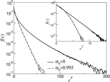
Figure 1: Rescaled velocity distribution $f(c)$ obtained by solving numerically the 1-D Boltzmann equation (1) with WN driving by the DSMC technique Bird for the strongly interacting so-called ’very hard particles’ model ($\nu=2$) ME ). Two extreme cases have been simulated, one close to perfect elasticity ($\alpha_{0}=0.995$) where the QE-tail $\ln f$ vs. $c^{\nu+2}$ (main frame) is visible, and the other at complete inelasticity ($\alpha_{0}=0$), where the standard tail $\ln f$ vs. $c^{1+\nu/2}$ (inset) is visible.

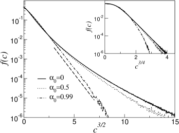
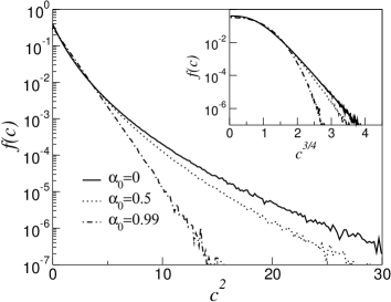
Figure 2: Left: Velocity distribution obtained from DSMC simulations for weakly interacting 1-D particles $(\nu=-\textstyle{\frac{1}{2}})$ with $\ln f(c)$ vs. $c^{\nu+2}$ (main frame) and vs. $c^{1+\nu/2}$ (inset). In the main frame the dashed line is a guide for the eye corresponding to the expected behavior (II). Right: $d=2$, $\ln f(c)$ vs $c^{2}$ (main) and vs. $c^{1+\nu/2}$ (inset).

III Negative Friction (NF) driving

The scaling equation for the analog of 4 with NF driving becomes,

$$I(c|f)=\frac{\gamma}{v_{0}^{\nu+1-\theta}}\frac{d}{dc}\left(c|c|^{\theta-1}f\right)=\frac{pq\kappa_{\nu}}{2\mu_{\theta+1}}\frac{d}{dc}\left(c|c|^{\theta-1}f\right).$$ (14)

Here $I(c|f)$ takes the form (9), and the analog of 5 has been used to eliminate $\gamma$. Moreover, $\mu_{\theta+1}=\langle|c|^{\theta+1}\rangle$ and $\kappa_{\nu}=\langle\langle|c-c_{1}|^{\nu+2}\rangle\rangle$. We therefore have to ${\cal O}(q)$ included,

$$f(c)\int dc_{1}|c-c_{1}|^{\nu}(c-c_{1})f(c_{1})=\frac{\kappa_{\nu}}{2\mu_{\theta+1}}c|c|^{\theta-1}f(c).$$ (15)

Previous studies of the free cooling regime of hard rods ($\theta=1,\,\nu=1$) have shown that $f(c)$ becomes singular when $\alpha_{0}\to 1^{-}$, and evolves into two symmetric Dirac peaks Mcnamara2 ; Sela ; Caglioti ; BBRTvW . It is indeed easy to check that $f(c)=[\delta(c+a)+\delta(c-a)]/2$ is a solution of 15), with $a=1/\sqrt{2}$ as required by our choice of normalization, $\langle c^{2}\rangle=1/2$, and $\kappa_{\nu}/(2\mu_{\theta+1})=2^{\nu}a^{\nu+1-\theta}$. Figure 3 shows that the approach to such a solution may be observed in the numerical simulations for $(\theta,\nu)\neq(1,1)$. In addition, one can check that $f(c)=A[\delta(c+a)+\delta(c-a)]+B\delta(c)$ is also a solution of Eq. (15), provided that $2A+B=1$ and $4Aa^{2}=1$ to enforce normalization. The DSMC results may indeed display such a three-peak structure (see Figure 4). Note that the parameters corresponding to Figures 3 and 4 are quite close: $(\theta,\nu)=(1.0,1.2)$ and (1.1, 1.3) respectively.

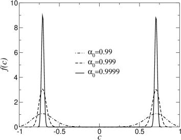
Figure 3: Velocity distribution obtained from DSMC simulations with NF driving for $(\theta,\nu)=(1.0,1.2)$ in 1-D. As $\varepsilon=1-\alpha_{0}\to 0^{+}$, $f(c)$ becomes increasingly peaked around $c=\pm c^{*}\equiv\pm 1/\sqrt{2}$, and ultimately evolves into two symmetric Dirac distributions. All distributions displayed here and in other figures are such that $\int dcf=1$, $\int dccf=0$ and $\int dcc^{2}f=1/2$.

However, upon changing the parameters $\theta$ and $\nu$, it appears that more complex shapes can be observed: $f(c)$ may evolve towards a 4-, 5-, 6-peaks form, or other structures such as displayed in Figure 5 where $f(c)$ seems to diverge at some points when $\alpha_{0}\to 1^{-}$, with nevertheless a finite support. The diversity of the various velocity distributions obtained numerically calls for a rationalizing study. By a combination of analytical work and numerical evidence, we will propose below a classification of the different possible limiting velocity distributions. In addition, in the double peak case, two natural questions will be addressed: Are the peaks exemplified in Figure 3 self-similar ? If so, what is their shape ?

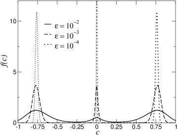
Figure 4: Same as Figure 3 for slightly different parameters ($\theta,\nu)=(1.1,1.3$). The velocity distribution now reaches a three-peak structure when $\varepsilon\equiv 1-\alpha_{0}\to 0^{+}$.

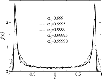
Figure 5: Velocity distribution obtained from DSMC for $(\theta,\nu)=(1.0,0.5)$. These parameters correspond to the border of the “Zoo” region shown in Figure 6.

III.1 The double peak scenario : structure and scaling

We start by looking for scaling solutions to Eq. (1), and restrict our analysis to the limiting form with the symmetric double peak. As in BBRTvW we take $f(c)$ of the doubly peaked form,

$$f(c)=\frac{b}{4E}\left[\psi\left(\frac{1+bc}{2E}\right)+\psi\left(\frac{1-bc}{2E}\right)\right],$$ (16)

where the width $E=q^{\omega}$ is expected to vanish when $q\to 0^{+}$ and $b$, $\omega$, together with the function $\psi$ are unknowns. We impose $\langle 1\rangle_{\psi}\equiv\int\psi=1$, and we choose $\langle x\rangle_{\psi}=0$, which together with the condition $\langle c^{2}\rangle=1/2$, implies $b^{2}=2(1+4E^{2}\langle x^{2}\rangle_{\psi})$, where normalization requires that $b\to({\sqrt{2}})^{-}$ as $q\to 0^{+}$. We note that asymmetric forms with $\psi(x)\neq\psi(-x)$ may be realized (see BBRTvW and later sections). The ansatz (16) allows us to resolve the structure of the Dirac peaks, shown in Figure 3, and to identify the type of self-similar behavior involved. However to this end, we need to expand the collision operator $I(c|f)$ to second order in the inelasticity $\varepsilon=1-\alpha_{0}=2q$. Restriction to first order, as done in (9), enables us to show that the double Dirac form is a solution of the Boltzmann equation, but does not allow us to impose constraints on the shape of $\psi$ and on the scaling exponent $\omega$. Technical details can be found in the appendix, where it is shown that the equation fulfilled by $\psi(x)$ reads,

$$q\psi^{\prime}(x)+2E^{2}(\nu+1-2\theta)x\psi(x)+2E^{\nu+2}\psi(x)\langle|x-y|^{\nu}(x-y)\rangle_{\psi}$$

$$-E^{3}\nu(\nu+1)\psi(x)(x^{2}+\langle y^{2}\rangle_{\psi})+2E^{3}\left[(\nu+1)(\nu+2)-2\theta(\theta+1)\right]\langle y^{2}\rangle_{\psi}\,\psi(x)$$

$$+4E^{3}\theta(\theta-1)x^{2}\psi(x)+2E^{\nu+3}\psi(x)\langle\langle|y-z|^{\nu+2}\rangle\rangle+{\cal O}(Eq\psi)=0,$$ (17)

where $y,z$ are dummy variables, and terms of ${\cal O}(Eq\psi)$ have been neglected. This relation involves terms of various orders in inelasticity. Given that $E=q^{\omega}$, these terms are ${\cal O}(q^{a})$ with $a=1,2\omega,(2+\nu)\omega,3\omega,(3+\nu)\omega,\omega+1$. Depending on the values of the parameters $\theta$ and $\nu$ one has to distinguish various possibilities to characterize the phase diagram, i.e. the physically allowed region of the $(\theta,\nu)$-parameter space. The stability criteria for the steady state (see ETB ) constrain the phase diagram in Figure 6 to be inside the region [$\theta\geq 0,\nu\geq\theta-1$].

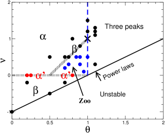
Figure 6: Phase diagram in the quasi-elastic limit. Each dot corresponds to a set of numerical simulations at smaller and smaller values of $\varepsilon=1-\alpha_{0}$, performed to check the validity of the scaling behaviors summarized in Table 1. The stability of the non-equilibrium steady state requires that $\nu>\theta-1$, while on the diagonal $\nu=\theta-1$ the velocity distribution has a power-law tail ETB . Here $\alpha$-, $\alpha^{\prime}$- and $\beta$-scalings are associated with a distribution with two Dirac peaks. For $\theta>1$ we observed numerically a solution with three Dirac peaks, while there does not seem to be a simple common feature for the distributions in the triangular “Zoo” region. An example of type $\alpha$-scaling is given in Figure 7 (See also Figure 8 for type $\beta$, and Figure 9 for type $\alpha^{\prime}$). Figures 12 and 13 together with Figure 5 above give an overview of several scaling shapes encountered in the Zoo region. The cross at (1,1) corresponds to the homogeneous cooling state of inelastic hard rods, explored in BBRTvW .

III.1.1 Case $\nu>0$ ($\alpha$- and $\beta$-scalings).

Type $\alpha$-scaling: The terms of order $q$ and $q^{2\omega}$ are the dominant ones in Eq. (17). So, $\omega=1/2$ and

$$\psi^{\prime}(x)=-(\nu+1-2\theta)x\psi(x).$$ (18)

The scaling function $\psi$ is therefore Gaussian,

$$\psi(x)\propto\exp\left(-(\nu+1-2\theta)x^{2}\right).$$ (19)

Such a solution is meaningful only if $\nu+1-2\theta>0$. This scaling behavior, hereafter referred to as type $\alpha$ (not to be confused with the restitution coefficient $\alpha_{0}$) is compared in Figure 7 with Monte Carlo results. The agreement between the analytical prediction and the numerical data involves two aspects : first, the exponent $\omega=1/2$ allows us to rescale all distributions onto a single master curve. Second, this curve is exactly of the form (19), where the prefactor hidden in the proportionality sign $\propto$ follows from normalization. Note that the excellent agreement between numerical data and analytical prediction is therefore obtained without any fitting parameter.

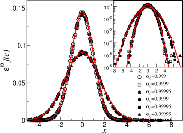
Figure 7: Scaling behavior of type $\alpha$. Plots of $\varepsilon^{\omega}f(c)$ vs. $x=(|c|-c^{*})/\varepsilon^{\omega}$ at $\theta=1$ for various inelasticities $\varepsilon=1-\alpha_{0}$ with $\omega=1/2$ as predicted. Here $c^{*}=1/\sqrt{2}$ corresponds to the peak of the distribution. Open symbols correspond to $\nu=1.5$ and filled symbols are for $\nu=1.2$ (same as in Figure 3). The inset shows the same results on a linear-log scale. In each case, the prediction of Eq. (19) for the scaling function is shown by the continuous curve. Note that no fitting parameter is involved.

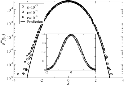
Figure 8: Scaling of type $\beta$. Same plot as Figure 7, displaying $\varepsilon^{\omega}f(c)$ vs. $x=(|c|-c^{*})/\varepsilon^{\omega}$ at $(\theta,\nu)=(3/4,1/2)$ with $\omega=1/(\nu+2)=2/5$ and $c^{*}=1/\sqrt{2}$. The continuous curve shows the prediction of Eq. (20) where the prefactor is determined from the constraint $\int dc\psi=1$.

Type $\beta$-scaling: On the line $\nu+1-2\theta=0$, the term of order $q^{2\omega}$ in (17) vanishes. If $0<\nu<1$, the terms $q$ and $q^{(\nu+2)\omega}$ can be balanced with the result $\omega=1/(\nu+2)$, and one finds at large $|x|$,

$$\psi(x)\propto\exp\left(-\frac{2}{\nu+2}|x|^{\nu+2}\right).$$ (20)

Unlike in $\alpha$-scaling , it is not possible here to obtain $\psi$ in close form. We will refer to (20) together with $\omega=1/(\nu+2)$ as a scaling of type $\beta$. Figure 8 shows that this behavior is in good agreement with the simulation results. Note that Eq. (20) seems to hold also for small values of $x$, whereas it is a priori only valid to describe the large$-x$ tail of $\psi$. We also note that the large$-x$ tail (20) exhibits the same exponent $\nu+2$ as in White Noise driving (see Eq. (11)). The important qualitative difference between the velocity distributions reported in section II and here is: with WN driving $f(c)$ is regular when $\alpha_{0}\to 1^{-}$, and with Negative Friction it develops singularities.

On the line $\nu+1-2\theta=0$, now with $\nu>1$, one can only balance the terms in $q$ and $q^{3\omega}$ in (17). This leads to $\omega=1/3$, but the associated function $\psi$ diverges for large arguments, and is thus unphysical. This is an indication that the double peak limiting form cannot be valid on the line $\nu+1-2\theta=0$ if $\nu>1$. Monte Carlo results confirm this. They display a limiting form with three peaks in this region of parameter space (see Figure 4 and section III.2 for a more thorough discussion, in particular Figure 6).

The special point on that line with $(\theta,\nu)=(1,1)$ represents free cooling of inelastic hard rods, which has been studied in BBRTvW . There it was shown that (16) holds, with $\omega=1/3$ and an asymmetric scaling function, behaving at large arguments as,

$$\psi(x) \simeq C\exp\left[\frac{1}{3}x^{3}+o(1)\right] \qquad(x\to-\infty)$$

$$\psi(x) \simeq C^{\prime}\exp\left[-2x\langle y^{2}\rangle_{\psi}\;+o(1)\right]\quad\hbox{with}\quad C^{\prime}\,=\,C\,\exp\left[-\frac{1}{3}\langle y^{3}\rangle_{\psi}\right] \qquad(x\to+\infty).$$ (21)

This asymmetry looks quite singular since most other scaling functions identified so far are symmetric. However, more exceptional cases with asymmetric scaling forms $\psi$ can be found in Figure 10 (which corresponds to the point $(0,-1)$, a case of marginal stability where $\nu=\theta-1$), as well as in the scaling shapes of the “Zoo” region of Figure 6. We also emphasize that the Dirac peaks appearing at the level of description when $\alpha_{0}\to 1^{-}$ are not artifacts of discarding any spatial dependence in (1), but provide the exact solution of the Boltzmann equation where due account is taken of the spatial degree of freedom of the particles. This has been confirmed in Caglioti and BBRTvW , where the velocity distributions of the homogeneous Boltzmann equation has been compared with its exact counterpart, obtained by Molecular Dynamics simulations.

III.1.2 Case $\nu=0$ ($\alpha^{\prime}$-scaling).

Type $\alpha^{\prime}$-scaling: When $\nu$ vanishes (Maxwell models), the first three terms on the rhs of (17) are of the same order, so that $\omega=1/2$ and $\psi$ satisfies,

$$\psi^{\prime}(x)+2(1-2\theta)x\psi(x)+2\psi(x)\langle x-y\rangle_{\psi}=\psi^{\prime}(x)+4(1-\theta)x\psi(x)=0,$$ (22)

since $\langle y\rangle_{\psi}=0$. Its solution is,

$$\psi(x)\propto\exp[-2(1-\theta)x^{2}].$$ (23)

This scaling, coined $\alpha^{\prime}$, a priori holds for $0\leq\theta\leq 1$, as follows from $\nu=0$ and the stability requirement $\nu+1-\theta\geq 0$. However, when $\theta=1$ (free cooling), (23) becomes unphysical. This is a consequence of the peculiar behavior of the freely cooling one-dimensional Maxwell model: the velocity distribution, which is algebraic, does not depend on $\alpha_{0}$ for $\alpha_{0}<1$ Maxwell ; Balda . In the (trivial) quasi-elastic limit, $f$ can consequently not develop a singularity of any kind. The scaling ansatz (16) has to break down for $\theta=1$, and it does. For $\theta<1$, the simulation data are in good agreement with $\alpha^{\prime}$-scaling predictions (see Figure 9), where again no fitting parameter has been used.

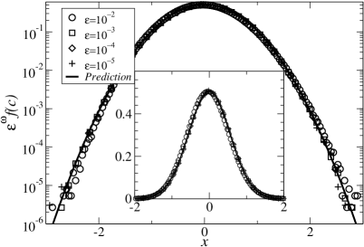
Figure 9: Scaling of type $\alpha^{\prime}$. Same plot as Figure 7 and Figure 8, displaying $\varepsilon^{\omega}f(c)$ vs. $x=(|c|-c^{*})/\varepsilon^{\omega}$ at $(\theta,\nu)=(0.2,0.0)$ with $\omega=1/2$ and $c^{*}=1/\sqrt{2}$. The continuous curve is for Eq. (23), i.e. $\propto\exp[-(1-\theta)x^{2})]$.

III.1.3 Case $\nu<0$ ($\beta$-scaling).

Type $\beta$-scaling: Finally we investigate the region $\nu<0$, which is further confined by the stability requirements for the steady state, $(\theta\geq 0,\nu\geq\theta-1)$. We then have $(2+\nu)\omega<2\omega$ and the terms of order $q$ and $q^{(2+\nu)\omega}$ balance each other in Eq. (17). This implies $\omega=1/(\nu+2)$ and

$$\frac{\psi^{\prime}(x)}{\psi(x)}=-2\langle|x-y|^{\nu}(x-y)\rangle_{\psi}.$$ (24)

We recover the $\beta$-scaling, and in particular the large$-|x|$ expression,

$$\psi(x)\propto\exp\left(-\frac{2}{\nu+2}|x|^{\nu+2}\right).$$ (25)

In the region $\nu<0$, we have successfully tested the validity of $\beta$-scaling against Monte Carlo simulations. In some cases however, we note that the best rescaling with respect to inelasticity is obtained with an exponent $\omega_{\text{opt}}$ that slightly differs from the predicted $1/(\nu+2)$. For instance, with $(\theta,\nu)=(0.7,-0.2)$ we find $\omega_{\text{opt}}\simeq 0.58$ while $1/(\nu+2)\simeq 0.55$. This could indicate that the scaling limit has not yet been reached, or it reflects the fact that for negative values of $\nu$, it is more difficult to reach the steady state in Monte Carlo simulations. Here the collision frequency is dominated by encounters with $|c_{1}-c_{2}|\ll 1$, that lead to a negligible change in the velocities of colliding partners. Consequently the numerical efficiency of our algorithm drops significantly.

III.2 Range of validity of scaling predictions: towards a phase diagram.

We have reported above a good agreement between DSMC calculations and the scaling predictions assuming the limiting double peak forms of $\alpha$-,$\beta$- and $\alpha^{\prime}$-scaling, when $\varepsilon=1-\alpha_{0}\to 0^{+}$, for several points in the ($\theta,\nu$)-plane. We have also shown that in some (complementary) regions of this plane the scaling hypothesis (16) does not provide an attracting fixed point solution of the stationary nonlinear Boltzmann equation (1) in the quasi-elastic limit. In fact, our analysis shows that physical solutions with $\alpha$-scaling do not exist for $\nu\geq 0$, and $\nu+1<2\theta$ (e.g. $(\theta,\nu)=(1.1,0.3);(1.1,1.1)$), and likewise for $\beta$-scaling with $\nu>1$ and $\nu+1=2\theta$ (e.g. $(\theta,\nu)=(1.1,1.2)$). In these regions we have no predictions.

Furthermore, in the triangular region $[\theta>1,\nu>1,\nu+1>2\theta]$ the NF driven kinetic equation admits – at least on the basis of the criteria developed – QE-limiting solutions with two peaks, consistent at least to second order in $\varepsilon$. The dynamics selects a different solution with three peaks (see Figure 4 with $(\theta,\nu)=(1.1,1.3)$).

A systematic Monte Carlo investigation of various points ($\theta,\nu$) –shown as dots in Figure 6– reveals that the range of validity of $\alpha$-scaling is in fact limited to $\theta\leq 1$ rque . In principle it would be possible to repeat the analysis of section III.1 with a three-peak solution, however we did not try to carry out this analysis. The reason is three-fold: First, it would not explain why $\alpha$-scaling is not selected by the dynamics in the angular region above. Second, it is cumbersome. Third, there is numerical evidence that $f(c)$ may differ from the two-peak or three-peak form (see the Zoo region of Figure 6). Thus, such analysis would in any case not provide a complete picture. A numerical investigation appears unavoidable and was used to identify the different regions of the “phase diagram” shown in Figure 6. We summarize our main findings:

• $\alpha$-Scaling holds for $\nu>0$ and $\nu>2\theta-1$ as found analytically, with the restriction $\theta\leq 1$ that follows from numerical evidence.

• $\beta$-Scaling applies to the line $0<\nu=2\theta-1<1$ and also to the region $\nu<0$, where the additional restriction $\nu>\theta-1$ follows from the stability requirement of the steady-state solution of Eq. (1). Figure 10 with $(\theta,\nu)=(0,-1)$ shows a case of marginal stability where $\nu=\theta-1$. It is observed that the scaling exponent is still given by $\omega=1/(\nu+2)$ but the form (25) breaks down ($\psi$ becomes asymmetric).

• $\alpha^{\prime}$-Scaling is valid on the “Maxwell” line $\nu=0$ for $\theta<1$.

• Hard rods under free cooling, i.e. $(\theta,\nu)=(1,1)$, display specific scaling (see Eq. III.1.1, Table 1 and Ref. BBRTvW for details).

• None of the above scalings hold for $\theta>1$, where we have always observed a triple peak as in Figure 4. Figure 11 (with the same parameters as Figure 4) shows that the distributions are also self-similar, with an exponent $\omega=1/2$. Although, we have no prediction for the three-peak forms, we note that the scaling function in Figure 11 is compatible with Eq. (19), pertaining to $\alpha$-scaling. This could be specific to the parameters chosen, since those value of $\theta$ and $\nu$ obey the inequalities, $\nu>0$ and $\nu>2\theta-1$, where $\alpha$-scaling provides a two-peak solution of the Boltzmann equation. Two- and three-peak shapes therefore seem to have common features. We did not explore self-similarity further in the three-peak region.

• There exists another triangular region in the ($\theta,\nu$)-plane (the Zoo in Figure 6), where $f(c)$ does not evolve toward a two-peak or a three-peak form. In some instances, the Monte Carlo data are compatible with a four-peak limit as $\varepsilon\to 0^{+}$ (see Figure 12 where only the sector with $c>0$ has been shown). In some other cases, we observe precursors of what seems to be a six-peak form (see Figure 13). For both Figures 12 and 13, it is difficult to decide if the limiting form for $\varepsilon\to 0^{+}$ will be a collection of Dirac distributions (with therefore a support of vanishing measure), or a distribution with finite support. We could however identify some points in the triangle where the limiting $f(c)$ clearly is of finite support (see Figure 5).

To summarize, $\alpha^{\prime}$- and $\beta$-scaling apply in the whole domain where they provide a solution to the Boltzmann equation, but $\alpha$-scaling has a restricted domain of relevance compared to the region where the corresponding solution is self-consistent. The key features of the analytical predictions are recalled in Table 1.

Scaling type	rescaling exponent	rescaling function
$\alpha$	$\omega=1/2$	$\psi(x)\propto\exp(-(\nu+1-2\theta)x^{2})$
$\alpha^{\prime}$	$\omega=1/2$	$\psi(x)\propto\exp(-2(1-\theta)x^{2})$
$\beta$	$\omega=1/(\nu+2)$	$\psi(x)\sim\exp(-2|x|^{\nu+2}/(\nu+2))$ at large $|x|$
$\theta=1,\nu=1$	$\omega=1/3$	Eq. (III.1.1), $\psi$ asymmetric

Table 1: Theoretical predictions for the different scaling behaviors in the two-peak region.

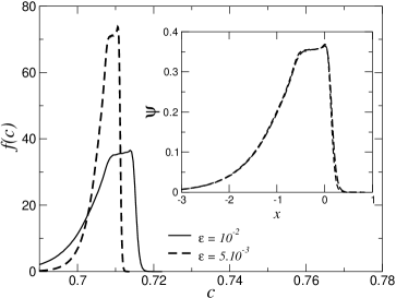
Figure 10: Velocity distribution at $(\theta,\nu)=(0,-1)$ for two inelasticities. $f(c)$ develops a cusp at $c=c^{*}$ where $c^{*}$ is $\varepsilon$-dependent. Plotting $\psi(x)=\varepsilon f(c)$ vs. $x=(c-c^{*})/\varepsilon$ (inset), shows that here the scaling form 16 applies with an asymmetric $\psi$, and $\omega=1=1/(\nu+2)$. For such low values of $\nu$, the CPU time required to gather statistical knowledge is particularly large.

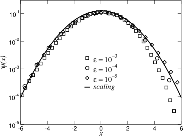
Figure 11: Plots of $\psi(x)=\varepsilon^{\omega}f(c)$ vs. $x=(c-c^{*})/\varepsilon^{\omega}$, with $\omega=1/2$ for the same parameters as in Figure 4 ($\theta,\nu)=(1.1,1.3)$, i.e. for $f(c)$ approaching a structure composed by three Dirac peaks. Here, $c^{*}\simeq 0.76$ denotes the position of the right peak seen in Figure 4. The continuous curve shows expression (19).

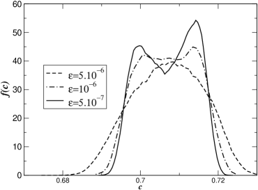
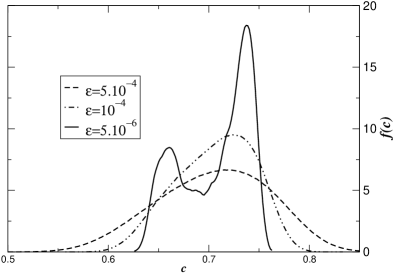
Figure 12: Two Zoo members at $(\theta,\nu)=(0.75,0.3)$ (left) and $(\theta,\nu)=(0.85,0.5)$ (right). Note the $x$- and $y$-scale in the plot on the right. For these parameters one needs to decrease $\varepsilon$ below $10^{-6}$ to realize that a seemingly single peak is likely to split into two sub-peaks as $\varepsilon\to 0^{+}$.

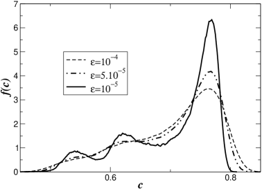
Figure 13: Another Zoo member at $(\theta,\nu)=(0.9,0.5)$. The velocity distribution seems to evolve towards a six-peak form as $\varepsilon\to 0^{+}$.

IV Conclusion

We have studied the one-dimensional nonlinear Boltzmann equation in the limit of quasi-elastic collisions for a class of dissipative fluids where material properties are encoded in an exponent $\nu$ such that the collision frequency between two particles with velocities $c_{1}$ and $c_{2}$ scales like $|c_{1}-c_{2}|^{\nu}$. Two driving mechanisms have been considered: stochastic white noise (in which case the generic effects only depend on $\nu$) and deterministic negative friction (in which case, in addition to $\nu$, a second important exponent $\theta\geq 0$, characterizing the driving, has been considered). In both stochastic and deterministic cases, the quasi-elastic limit does not commute with the limit of large velocities. This is specific to one space dimension. There are however important differences between the two driving mechanisms. In the white noise case, the normalized velocity distribution $f(c)$, suitably rescaled to have fixed variance, is regular and displays stretched exponential QE-tails of the form $\exp[-c^{\nu+2}]$. On the other hand, $f(c)$ with deterministic driving –which encompasses the much studied homogeneous cooling regime– develops singularities as $\varepsilon\equiv 1-\alpha_{0}\to 0^{+}$. The corresponding scaling behavior is particularly rich. We have classified the scaling forms encountered in several families, see Figure 6 for a global picture. Some regions of this $(\theta,\nu)$-diagram are well understood, such as regions $\alpha$, $\alpha^{\prime}$ and $\beta$. Some other domains resist theoretical understanding. Even if some progress might be possible in the three-peak region (one at $c=0$, the two others at $\pm c^{*}$), the situation in the central Zoo region of Figure 6 seems more difficult to rationalize, and computationally elusive, since one needs to reach extremely small values of $\varepsilon$ to see the precursors of presumed singularities.

Appendix A

In this appendix, we expand the collision operator $I(c|f)$ defined in (7) in powers of $q=(1-\alpha)/2$, up to second order. Such an expansion is required to unveil the internal structure of the singular peaks that develop as $q\to 0^{+}$ with driving by negative friction. Assuming that the functional form of the velocity distribution is given by (16), our goal is to obtain here the differential equation fulfilled by the scaling function $\psi$. Starting from

$$I(c|f)=\int du|c-u|^{\nu}f(u)\left[\frac{1}{p^{\nu+1}}f\left(c+\frac{q}{p}(c-u)\right)-f(c)\right],$$ (26)

one obtains by extending 9 to ${\cal O}(q^{2})$ included,

$$I(c|f)=q\frac{d}{dc}\left[f(c)\int duf(u)|c-u|^{\nu}(c-u)\right]+\frac{q^{2}}{2}\left(\frac{d}{dc}\right)^{2}\left[f(c)\int du|c-u|^{\nu+2}f(u)\right]+{\cal O}(q^{3}).$$ (27)

Inserting the ansatz (16) into (27), the term $I^{(1)}$ of order $q$ reads

$$I^{(1)}=-q\left(\frac{b}{4E}\right)^{2}\left(\frac{2}{b}\right)^{\nu+1}\frac{d}{dx}\left\{\psi(x)\int dy\psi(y)(1-E(x+y))^{\nu+1}\right\}$$

$$+q\left(\frac{b}{4E}\right)^{2}\left(\frac{2E}{b}\right)^{\nu+1}\frac{d}{dx}\left\{\psi(x)\int dy\psi(y)|x-y|^{\nu}(x-y)\right\},$$ (28)

and expanding $(1-E(x+y))^{\nu+1}$ further yields,

$$I^{(1)}=\frac{q}{4E^{2}}\left(\frac{2}{b}\right)^{\nu-1}\frac{d}{dx}\left\{\left[-1+xE(\nu+1)-\frac{\nu(\nu+1)}{2}E^{2}\int dy\psi(y)(x+y)^{2}+E^{\nu+1}\int dy\psi(y)|x-y|^{\nu}(x-y)\right]\psi(x)\right\}.$$ (29)

The second order term $I^{(2)}$ in (27) is

$$I^{(2)}=\frac{q^{2}}{2}\left(\frac{b}{4E}\right)^{2}\frac{b}{2E}\left(\frac{d}{dx}\right)^{2}\left\{\left(\frac{2E}{b}\right)^{\nu+2}\psi(x)\int dy\psi(y)|x-y|^{\nu+2}+\left(\frac{2}{b}\right)^{\nu+2}\psi(x)\int dy\psi(y)|1-E(x+y)|^{\nu+2}\right\}$$ (30)

and we can keep only the largest term as $q\to 0^{+}$, i.e.

$$\frac{q^{2}}{8E^{3}}\left(\frac{2}{b}\right)^{\nu-1}\psi^{\prime\prime}(x).$$ (31)

Collecting terms yields finally,

$$I(c|f)=\frac{q}{4E^{2}}\left(\frac{2}{b}\right)^{\nu-1}\frac{d}{dx}\left\{\left[-1+xE(\nu+1)-\frac{\nu(\nu+1)}{2}E^{2}\int dy\psi(y)(x+y)^{2}\right.\right.$$

$$\left.\left.+E^{\nu+1}\int dy\psi(y)|x-y|^{\nu}(x-y)\right]\psi(x)+\frac{q}{2E}\psi^{\prime}(x)\right\}.$$ (32)

The next step is to evaluate the right hand side of equation (14), by an expansion of the moments $\kappa_{\nu}$ and $\mu_{\theta+1}$,

$$\mu_{\theta+1} = \int dc|c|^{\theta+1}f(c)=\int dy\psi(y)\left|\frac{1-2Ey}{b}\right|^{\theta+1}$$ (33)

$$= b^{-1-\theta}[1+2\theta(\theta+1)E^{2}\langle y^{2}\rangle_{\psi}]$$

$$\kappa_{\nu} = \int\int dcdu|c-u|^{\nu+2}f(c)f(u)$$

$$= \frac{2^{\nu+1}}{b^{\nu+2}}\left[\int dydz\psi(y)\psi(z)(1-E(y+z))^{\nu+2}+E^{\nu+2}\int dydz\psi(y)\psi(z)|y-z|^{\nu+2}\right]$$

$$= \frac{2^{\nu+1}}{b^{\nu+2}}\left[1+(\nu+1)(\nu+2)E^{2}\langle y^{2}\rangle_{\psi}+E^{\nu+2}\int dydz\psi(y)\psi(z)|y-z|^{\nu+2}\right].$$ (35)

With $c$ close to $-1/b$, one can also perform the expansion

$$\frac{d}{dc}\left(c|c|^{\theta-1}f\right)=-\frac{b^{2-\theta}}{8E^{2}}\frac{d}{dx}\left\{\psi(x)[1-2\theta Ex+2\theta(\theta-1)E^{2}x^{2}],\right\}$$ (36)

and the rhs of equation (16) can thus finally be written as

$$pq\frac{\kappa_{\nu}}{2\mu_{\theta+1}}\frac{d}{dc}\left(c|c|^{\theta-1}f\right)=-\frac{pq}{4E^{2}}\left(\frac{2}{b}\right)^{\nu-1}\frac{d}{dx}\left\{\psi(x)[1-2\theta Ex+2\theta(\theta-1)E^{2}x^{2}\right.$$ (37)

$$+\left.((\nu+1)(\nu+2)-2\theta(\theta+1))E^{2}\langle y^{2}\rangle_{\psi}+E^{\nu+2}\int\int dydz|y-z|^{\nu+2}\psi(y)\psi(z)]\right\}$$ .

We obtain (17), after simplification by the prefactors and integration with respect to $x$.

References

- (1) I. Goldhirsch, Ann. Rev. Fluid Mech. 35, 267 (2003).
- (2) Theory of Granular Gas Dynamics, Th. Pöschel and N.V. Brilliantov (Eds), (Springer-Verlag, Berlin, 2003).
- (3) A. Barrat, E. Trizac, M.H. Ernst, J. Phys. Condens. Matter 17, S2429 (2005).
- (4) S. McNamara and W.R. Young, Phys. Fluids A 5, 34 (1993).
- (5) D. Benedetto, E. Caglioti and M. Pulvirenti, Math. Mod. and Num. An. 31, 615 (1997).
- (6) D. Benedetto, E. Caglioti, J.A. Carrillo and M. Pulvirenti, J. Stat. Phys. 91, 979 (1998).
- (7) R. Ramirez and P. Cordero, Phys. Rev. E 59, 656; also in Granular Gases, eds T. Poschel and S. Luding (Springer, NY, 2001).
- (8) S. McNamara and W.R. Young, Phys. Fluids A 4, 496 (1992).
- (9) N. Sela and I. Goldhirsch, Phys. Fluids 7, 507 (1995).
- (10) E. Ben-Naim, S.Y. Chen, G.D. Doolen and S. Redner, Phys. Rev. Lett. 83, 4069 (1999).
- (11) A. Rosas, D. ben-Avraham and K. Lindenberg, Phys. Rev. E 71, 032301 (2005).
- (12) M.H. Ernst and R. Brito, Phys. Rev. E 65, 040301(R) (2002).
- (13) M.H. Ernst, E. Trizac and A. Barrat, J. Stat. Phys. 124, 549 (2006).
- (14) M.H. Ernst, E. Trizac and A. Barat, Europhys. Lett. 76, 56 (2006).
- (15) D.R.M. Williams and F.C. MacKintosh, Phys. Rev. E 54, R9 (1996); G. Peng and T. Ohta, Phys. Rev. E 58, 4737 (1998); T.P.C. van Noije and M.H. Ernst, Granular Matter 1, 57 (1998); C. Henrique, G. Batrouni and D. Bideau, Phys. Rev. E 63 011304 (2000); S.J. Moon, M.D. Shattuck and J.B. Swift, Phys. Rev. E 64 031303 (2001); I. Pagonabarraga, E. Trizac, T.P.C. van Noije and M.H. Ernst, Phys. Rev. E 65, 011303 (2002); J.S. van Zon and F.C. MacKintosh, Phys. Rev. E 72, 051301 (2005).
- (16) J.M. Montanero and A. Santos, Granular Matter 2, 53 (2000).
- (17) A. Barrat, T. Biben, Z. Ràcz, E. Trizac and F. van Wijland, J. Phys. A: Math. Gen. 35, 463 (2002).
- (18) A Santos and M.H. Ernst, Phys. Rev. E 68, 011305 (2003).
- (19) M.H. Ernst, Physics. Reports 78, 1 (1981).
- (20) E. Ben-Naim and P.L. Krapivsky, Phys. Rev. E 61, R5 (2000); E. Ben-Naim and P.L. Krapivsky, Phys. Rev. E 66, 1309 (2002).
- (21) A. Baldassarri, U.M.B. Marconi, and A. Puglisi, Europhys. Lett. 58, 14 (2002); A. Baldassarri, U.M.B. Marconi, and A. Puglisi, Math. Mod. Meth. Appl. S. 12, 965 (2002).
- (22) M.H. Ernst and R. Brito, J. Stat. Phys. 109, 407 (2002).
- (23) G. Bird, Molecular Gas Dynamics and the Direct Simulation of Gas Flows (Clarendon, Oxford, 1994).
- (24) In this respect, Figure 7 corresponds to the frontier of the domain of validity of -scaling. We have checked however that cases with and belong to the family, provided that .