Transport of fractional Hall quasiparticles through an antidot

Abstract

Current statistics of an antidot in the fractional quantum Hall regime is studied for Laughlin’s series. The chiral Luttinger liquid picture of edge states with a renormalized interaction exponent $g$ is adopted. Several peculiar features are found in the sequential tunneling regime. On one side, current displays negative differential conductance and double-peak structures when $g<1$. On the other side, universal sub-poissonian transport regimes are identified through an analysis of higher current moments. A comparison between Fano factor and skewness is proposed in order to clearly distinguish the charge of the carriers, regardless of possible non-universal interaction renormalizations. Super-poissonian statistics is obtained in the shot limit for $g<1$, and plasmonic effects due to the finite-size antidot are tracked.

I Introduction

The peculiar properties of quasiparticles (qp) in the fractional quantum Hall effect (FQHE) have received great attention especially for the states at filling factor $\nu=1/p,\,p$ odd integer, in which gapped bulk excitations were predicted to exist and to possess fractional chargeLaughlin $e^{*}=\nu e$ ($e<0$ electron charge) and statistics.HalperinArovas

A boundary restriction of this theory was subsequently put forward in terms of edge states by Wen.Wen This theory recovered the fractional numbers of quasiparticles in the framework of chiral Luttinger Liquids ($\chi$LL), and indicated tunneling as an accessible tool to probe them.kanefisher Accordingly, quasiparticles with charge $e/p$ were measured in shot noise experiments with point contact geometries and edge-edge backscattering.depicciotto

A key prediction of $\chi$LL theories is that the interaction parameter should be universal and equal to $\nu$. As a consequence, the quasiparticle (electron) local tunneling density of states obeys a power law in energy $D\propto E^{\nu-1}$ ($D\propto E^{1/\nu-1}$). Several geometries have been set up in experiments to test this nonlinearity through measurements of tunneling current $I$ versus bias voltage $V$. For instance, in the case of electron tunneling between a metal and an edge at filling $\nu$, one should have $I\propto V^{\alpha}$ in the limit $eV\gg k_{B}T$ with $\alpha=1/\nu$.kanefisher Experimentschang at filling factor $1/3$ indeed proved a power-law behaviour but with $\alpha\neq 3$. Deviations were observed also with quasiparticle tunneling in an almost open point contact geometry at $\nu=1/3$;chung here, the predicted backscattering linear conductance is $G_{B}\propto T^{2\nu-2}$ while the measured quantity obeys a power law with positive exponent. Analogous discrepancies were observed in a similar geometry, with the quasiparticle tunneling differential conductance developing a minimum around zero bias instead of a maximum for decreasing temperature.beltram Moreover, several numerical calculations and simulations also disagree with the conventional chiral Luttinger theories. We mention for instance finite-size exact-diagonalization calculations with short-rangezuelicke or Coulomb electron-electron interactionstsiperg ; goldmant ; cheianov and Monte Carlo simulations with interacting Composite Fermions on a ring.mandaljain

The disagreements of $\chi$LL predictions with observed exponents are still not completely understood, although several theoretical mechanisms have been put forward to reproduce a renormalized Luttinger parameter, including coupling to phonons or dissipative environments,halpros ; eggert ; khlebnikov ; levitov effects of interaction range,papa ; evers edge reconstruction with smooth confining potentials.yang ; wan ; joglekar ; papa2

Our purpose is to discuss fractional Hall edges in an enriched $\chi$LL theory where the possibility of a renormalized interaction parameter $g\neq\nu$ is assumed, analysing different transport regimes and clearly distinguishing signatures of charge $\nu e$ qp from effects due to the quasiparticle propagators governed by $g$. To do so, we choose a geometry where two fractional quantum Hall edges are connected via weak tunneling through an edge state encircling an antidot as in Fig. 1.Geller97 ; merlo Such a setup has proven to be extremely versatile and controllable. It has been for instance employed in a series of experiments where fractional charge and statistics of quasiparticles were addressed.gold The same geometry has been also used to detect blockade effects and Kondo physics with spinful edges in the integer regime.cavendish

As mentioned before, a series of experimental observations of fractional charge has been based on noise measurements:depicciotto the possibility to extract a significant $e^{*}/e$ from such measurements is given by the fact that the geometry of the setup and the tunneling regime ensure a poissonian process. Smooth evolution in the charge carrier at $\nu=1/3$ from $e^{*}=\nu e$ to $e$ was observed in point contacts changing the backscattering amplitude via gates from 0 to 1.griffiths This appears consistent with evolution from fractional qp to electron tunneling.kanefisher92 Anyway, this conclusion can only be obtained under the additional hypothesis of independent particle tunneling.nota4 Only the observation of higher moments, as e.g. the normalized skewness, could cross-check this hypothesis.saleurweiss Therefore, to fully explain the charge measurements one has to observe higher moments beyond the Fano factor. Recent advances in measurement techniques could open this intriguing possibility, especially in view of the unexpected results recently reported.chung ; beltram

In this paper we propose to compare Fano factor and skewness in transport regimes where the statistics of the charge transfer is not poissonian. We focus our attention on transport through an antidot in weak-backscattering and sequential tunneling limit, at fractional filling factor $\nu=1/p$ ($p$ odd integer). Our task is twofold: on one side, we analyse the tunneling current. It presents remarkable features driven by $g$, like e.g. negative differential conductance and double-peak structures. Power-law behaviours exist and can be used to determine the renormalized interaction parameter. On the other side, we derive a method to assess fractional charge independently of possibly renormalized $g\neq\nu$. We analyse noise and skewness in processes with different transport statistics both in the shot and in the thermal limit. We find universal points that unambiguously define the fractional charge. In addition, we describe transport regions where the Fano factor is sensitive to the power laws of the quasiparticle propagators and presents super-poissonian correlations.

The paper is organized as follows: in Sec. II the model is introduced and bosonization procedures are briefly reviewed. Sections III and IV contain the description of methods and results. Finally, in Sec. V we discuss our findings and comment existing experimental applications.

II model

Figure 1: Geometry of the system. In white, the Hall fluid; in black, the depleted areas defining the two quasiparticle tunneling points between the left ($L$) or right ($R$) edge and the antidot ($A$). In this setting, the magnetic field points out of the plane.

In our model, edge states form at the boundaries of the sample and around the antidot (Fig. 1); mesoscopic effects are associated to the finite size of the antidot through an Aharonov-Bohm (AB) coupling, and tunneling barriers couple the circular antidot with both edges. The complete Hamiltonian reads

$$H=H^{0}_{{L}}+H^{0}_{{R}}+H^{0}_{{A}}+H^{\rm AB}+H_{R}^{{T}}+H_{L}^{{T}},$$ (1)

and the individual pieces are now described in detail.

II.1 Bosonization of free Hamiltonians

In Eq. (1), $H^{0}_{l}$ are standard Wen’s hydrodynamical Hamiltonians for the left, right and antidot edge ($l=L,R,A$): in terms of the electron excess density $\rho_{l}(x)$ ($\hbar=1$), one hasGeller97 ; merlo ; kette97

$$H_{l}^{0}=\frac{\pi v}{\nu}\int_{-\mathcal{L}_{l}/2}^{\mathcal{L}_{l}/2}\!\!\!\mathrm{d}x\,\rho^{2}_{l}(x),$$ (2)

where $v$ is the edge magnetoplasmon velocity and ${\mathcal{L}}_{l}$ is the edge length. The theory is bosonized with the prescription $\rho_{l}(x)=\partial_{x}\phi_{l}(x)/2\pi$ where $\phi_{l}(x)$ are scalar fields comprising both a charged and a neutral sector:

$$\phi_{l}(x)=\phi_{l}^{0}(x)+\phi_{l}^{p}(x).$$ (3)

The direction of motion of the fields is fixed by the external magnetic field. Here we chose for convenience to set curvilinear abscissas in such a way that all fields have the same chirality (right movers). The periodic neutral plasmonic mode for the edge $l$ is

$$\phi_{l}^{p}(x)=\sum_{{k_{l}}>0}\sqrt{\frac{2\pi\nu}{k_{l}\mathcal{L}_{l}}}(a_{l,{k_{l}}}e^{ik_{l}x}+a_{l,{k_{l}}}^{\dagger}e^{-ik_{l}x})e^{-k_{l}a/2},$$ (4)

where $a$ is an ultraviolet cutoff and bosonic creation and annihilation operators obey $[a_{i,k},a_{j,k^{\prime}}^{\dagger}]=\delta_{ij}\delta_{kk^{\prime}}$ with a quantized wavevector $k_{l}=m\frac{2\pi}{\mathcal{L}_{l}}$, $m\in\mathbb{N}$. The charged zero mode reads

$$\phi_{l}^{0}(x)=\frac{2\pi}{\mathcal{L}_{l}}\nu n_{l}x-\chi_{l}$$ (5)

with $n_{l}$ the excess number of quasiparticles and $\chi_{l}$ an Hermitian operator conjugate to $n_{l}$. The canonical commutation relation $[\chi_{j},n_{l}]=i\delta_{jl}$ together with $[\phi_{j}^{0}(x),\phi_{l}^{p}(x^{\prime})]=0$ ensure that the field on each edge satisfies

$$[\phi_{l}(x),\phi_{l}(x^{\prime})]=i\pi\nu\,{\rm sgn}\,(x-x^{\prime}).$$ (6)

Charge $\nu$ quasiparticle fields are now defined through exponentiation,

$$\psi_{l}(x)=\frac{1}{\sqrt{2\pi a}}e^{i\phi_{l}(x)}e^{i\pi\nu x/\mathcal{L}_{l}},$$ (7)

where the extra phase has been added to preserve the correct twisted boundary conditionsfradkin for the qp field, $\psi_{l}(x+\mathcal{L}_{l})=\psi_{l}(x)e^{i2\pi n_{l}\nu}$. Equation (6) guarantees that the fields $\psi_{l}$ create fractional charge excitations. The same commutation relation also insures that quasiparticles have fractional statistics

$$\psi_{l}(x)\psi_{l}^{\dagger}(x^{\prime})=\psi_{l}^{\dagger}(x^{\prime})\psi_{l}(x)e^{i\pi\nu\,{\rm sgn}\,(x-x^{\prime})}.$$ (8)

For quasiparticles of different edges, fractional statistics is introduced with suitable commutation relations $[\chi_{j},\chi_{l}]=i\pi\nu\,{\rm sgn}\,(w_{j}-w_{l})$ with $w_{R}=-w_{L}=1$ and $w_{A}=0$.

With prescriptions (4) and (5), Eq. (2) becomes

$$H^{0}_{{l}}=E_{\rm c}^{l}n_{l}^{2}+\sum_{s=1}^{\infty}s\epsilon_{l}a_{l,s}^{\dagger}a_{l,s},$$ (9)

where $E_{\rm c}^{l}=\pi\nu v/\mathcal{L}_{l}$ is the topological charge excitation energy; for the neutral sector, $\epsilon_{l}=2\pi v/\,\mathcal{L}_{l}$ is the plasmonic excitation energy.

The total excess charge on an edge is given by

$$Q_{l}=e\int_{-\mathcal{L}_{l}/2}^{\mathcal{L}_{l}/2}\!\!\!\mathrm{d}x\,\frac{\partial_{x}\phi_{l}(x)}{2\pi}=n_{l}e^{*},$$ (10)

and is conserved in the absence of tunneling.

Finally, the limit $\mathcal{L}_{L},\mathcal{L}_{R}\to\infty$ is taken. In the following, for brevity’s sake, we relabel the antidot variables as $\mathcal{L}=\mathcal{L}_{A}$, $\epsilon=\epsilon_{A}$, $E_{\rm c}=E_{\rm c}^{A}$ and $n=n_{A}$.

II.2 Aharonov-Bohm coupling

The Hamiltonians Eq. (2) are expected to describe the system anywhere on a $\nu=1/p$ plateau since they are based on incompressibility. Nevertheless the antidot edge, encircling a finite area, is sensitive to the actual position in the plateau through a coupling to the Aharonov-Bohm (AB) flux.GellerLoss2 ; gold We model this effect with an extra magnetic field pointing in the opposite direction with respect to the background magnetic field.nota3 The AB vector potential along the antidot edge reads $|\vec{A}|=\frac{\Phi}{\mathcal{L}}$ where $\Phi$ is the AB flux of the additional magnetic field. The Aharonov-Bohm coupling is $H^{\rm AB}\propto\vec{j}\cdot\vec{A}$ and describes the coupling of the antidot current density with $\vec{A}$. By a gauge transformation, it is easy to seeGeller97 that this amounts simply to a shift in the energies in $H^{0}_{{A}}$ in Eq. (9) according to $E_{\rm c}n^{2}\to E_{\rm c}(n-\Phi/\Phi_{0})^{2}$, where $\Phi_{0}=hc/|e|$ is the flux quantum.

II.3 Tunnel coupling

Each $\chi$LL supports several excitations other than the single quasiparticle Eq. (7), given in general by $\psi_{l}^{m}(x)\propto\exp[im\phi_{l}(x)],\,m\in\mathbb{N}$. The electron corresponds to $m=1/\nu$, while the single quasiparticle fields $\psi_{j}(x)$ are obtained by setting $m=1$. One should therefore consider all possibilities for tunneling, i.e. all terms like $t^{(m)}{\psi_{A}^{m}}^{\dagger}(x)\psi_{j}^{m}(x)$, $j=L,R$.

Renormalization group (RG) flow equations have been set up for the antidot geometry in Ref. GellerLoss2, . Here we remind that the renormalized $m$-quasiparticle tunneling amplitude $t^{(m)}_{\rm ren}$ scales as a power law

$$t^{(m)}_{\rm ren}=\left(\frac{a_{\rm ren}}{a}\right)^{1-m^{2}g}t^{(m)}$$ (11)

under increase in the unit-cell size $a\to a_{\rm ren}$. Considering e.g. $g=1/3$, the single-qp tunneling amplitude $t^{\rm qp}=t^{(1)}_{\rm ren}$ diverges when scaling to lower energies, while the electron amplitude $t^{e}=t^{(3)}_{\rm ren}$ scales to zero. The largest $a_{\rm ren}$ attainable is the minimum between the thermal length $\propto v/T$ and the antidot length $\mathcal{L}$. A crossover temperature $k_{\rm B}T_{0}\sim E_{\rm c}=\pi\nu v/\mathcal{L}$ exists such that for $T>T_{0}$ one has $t^{(m)}_{\rm ren}/t^{(m)}\propto T^{m^{2}g-1}$, while for $T<T_{0}$ the flow is cutoff by the energy associated to the finite size of the antidot $t^{(m)}_{\rm ren}/t^{(m)}\propto E_{\rm c}^{m^{2}g-1}$. In the following we will assume $k_{\rm B}T\ll E_{\rm c}$ and bare tunneling amplitudes such that electron tunneling can be neglected. Indeed this appears to be the case in most experimental observations where single quasiparticle tunneling is clearly observed.gold We therefore only retain the dominant term

$$H^{T}=\sum_{j=L,R}H^{{T}}_{j}=v\sum_{j=L,R}\left(t_{{j}}\psi_{{A}}^{\dagger}(x_{j})\psi_{{j}}(0)+h.c.\right),$$ (12)

that represents the single-quasiparticle tunneling between the infinite edges and the antidot. Here the velocity $v$ is introduced to have dimensionless tunneling amplitudes $t_{j}$.

A finite source-drain voltage $V$ is applied between the left and right edges, producing a backscattered tunneling current $I(t)$ of quasiparticles through the antidot

$$I(t)=\left[\dot{Q}_{L}(t)-\dot{Q}_{R}(t)\right]/2,$$ (13)

with $\dot{Q}_{j}(t)=i[Q_{j},H]=-ie^{*}v[t_{j}\psi_{{A}}^{\dagger}(x_{j},t)\psi_{{j}}(0,t)-h.c.]$ and $j=L,R$. We will consider asymmetric voltage drop with $\alpha V$ and $(1-\alpha)V$ the voltage drops across the left and right barrier and $0<\alpha<1$ (see Fig. 2a)).

III Method

III.1 Sequential tunneling rates

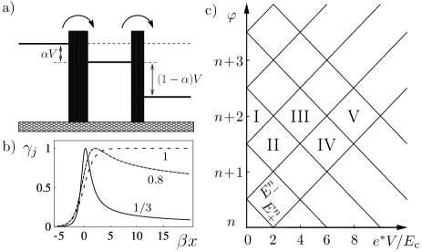
Figure 2: a) Double-barrier system, with the voltage drop $\alpha V$ [$(1-\alpha)V$)] on the left [right] barrier. The forward transitions, corresponding to qp transfers contributing positively to the current, are indicated. b) Plot of $\gamma_{j}(x)$ in Eq. (19) as a function of $\beta x$ for $g=1/3,0.8,1$, in units $|t_{j}|^{2}(\omega_{c}/4\pi^{2})(\beta\omega_{c}/2\pi)^{1-g}/\mathbf{\Gamma}(g)$ and normalized to its maximum value. c) Scheme of transport regions in the $(V,\varphi)$ plane. Roman numbers indicate the number of charge states involved in the transport. Thin lines signal the onset of transitions, where energies $E_{\pm}^{n}=0$(see Eq. (III.3)).

For small tunneling as compared with temperature, transport can be safely described within the sequential tunneling regime.furusaki Here, the main ingredients are the incoherent tunneling rates $\Gamma_{L,R}(E)$. They are obtained from the transition probability between the antidot state with $n$ qp at time $0$ and the state with $n^{\prime}$ qp at time $t$, at second order in the tunneling HamiltonianbraggioEPL

$$\Gamma_{j}(E)=\left(\frac{v}{2\pi a}\right)^{2}|t_{j}|^{2}\int_{-\infty}^{+\infty}\mathrm{d}\tau e^{-W_{A}(\tau)}e^{-W_{j}(\tau)}e^{i\tau E},$$ (14)

where

$$W_{l}(t)=-\langle\phi_{l}^{p}(x,t)\phi_{l}^{p}(x,0)\rangle+\langle\phi_{l}^{p}(x,0)\phi_{l}^{p}(x,0)\rangle$$ (15)

are the thermal correlation functions for the edge ($L,R$) and antidot ($A$) plasmonic excitations. They can be cast in the standard dissipative formbraggioEPL

$$W_{l}(t)=\int_{0}^{\infty}\!\!\!\mathrm{d}\omega\frac{J_{l}(\omega)}{\omega^{2}}\left(\left(\cos\omega t-1\right)\coth\frac{\beta\omega}{2}-i\sin\omega t\right)$$ (16)

with the antidot and lead spectral densities

$$J_{A}(\omega) = \tilde{g}\omega\epsilon\sum_{s=1}^{\infty}\delta(\omega-s\epsilon)e^{-\omega/\omega_{c}}$$ (17a)

$$J_{L,R}(\omega) = g\omega e^{-\omega/\omega_{c}}$$ (17b)

where $\omega_{c}=v/a$ is a high energy cut-off and $\beta=1/k_{\rm B}T$. It is important to observe that this expression holds with the assumption that the plasmonic fields $\phi_{l}^{p}$ are fully relaxed to thermal equilibrium. Mechanisms that could guarantee this assumption include for instance thermalizing interactions with external degrees of freedom. In the standard $\chi$LL theory $g=\tilde{g}=\nu$ for all edge fields. Here we consider the possibility that $g,\tilde{g}\neq\nu$ to describe renormalization effects.

In the present paper, we do not enter into a microscopical derivation of exponents and only assume phenomenologically that renormalization of exponents takes place. The functional form of the quasiparticle correlators is thus preserved but is governed by a parameter $g=\nu F$. The explicit value of $F$ will depend on the details of interaction, and we will consider it as a parameter.

Several mechanisms have been proposed to account for renormalization. A striped phase is analysed in Ref. halpros, , where interaction is assumed between a $\nu=1/p$ $\chi$LL and phonon-like excitations carrying no net electric current. No tunneling of charge takes place between the $\chi$LL and the extra phonon modes, nor between the latter and the contacts. This assumptions are relevant in the case of tunneling between two edge states across a Hall liquid, as in the weak backscattering limit of the point-contact geometry or of our edge-antidot-edge setup. The only role of the additional modes is a modification of the backscattering dynamics between two chiral edges, leading to a renormalized exponent $g=\nu F$, where $F>1$ is a function of the coupling strength and of the phonon sound velocity.

Another possibility for tunneling renormalization relies on density-density interactions between chiral edge states in a split Hall bar geometry, with parameters $g_{1}$ and $g_{2}$ describing respectively coupling across the constriction and across the Hall bar.papa Correlation functions for quasiparticles can be calculated exactly in this model and give rise to an interedge tunneling current governed by $g=\nu F$, where now $F$ depends on $g_{1}$ and $g_{2}$.

Other proposals have been put forward and point toward more profound modifications of standard chiral Luttinger Liquids. Interactions with phonons have been considered, causing the bosonic field $\phi$ to split into several normal modes.eggert ; khlebnikov Edge reconstruction offers a further scenario, with a non-monotonic density profile of the two-dimensional Hall droplet near the edge essentially induced by electrostatics.evers ; goldmant ; joglekar ; tsiperg ; wan ; yang

We now return to the expression of the rates Eq. (14). It is well known within the bosonized description of edge states and readsGellerLoss2 ; braggio ; braggioEPL ; matson

$$\Gamma_{j}(E)=\sum_{s=-\infty}^{+\infty}w_{s}\gamma_{j}(E-s\epsilon),$$ (18)

where

$$\gamma_{j}(x)=|t_{j}|^{2}\frac{\omega_{c}}{(2\pi)^{2}}\left(\frac{\beta\omega_{\rm c}}{2\pi}\right)^{1-g}\frac{|\mathbf{\Gamma}(g/2+i\beta x/2\pi)|^{2}}{\mathbf{\Gamma}(g)}e^{\beta x/2}$$ (19)

with $\mathbf{\Gamma}(x)$ the Euler Gamma function. The sum in Eq. (18) represents the contribution of plasmons, with weight factors $w_{s}$.braggioEPL At $T=0$ they are

$$w_{s} = \frac{\mathbf{\Gamma}(\tilde{g}+s)}{\mathbf{\Gamma}(\tilde{g})s!}\left(\frac{\epsilon}{\omega_{c}}\right)^{\tilde{g}}e^{-s\epsilon/\omega_{c}}\Theta(s),$$ (20)

with $\Theta(s)$ the Heaviside step function.

It is apparent that the rates have contributions from both the edge and the antidot correlators. Their functional behaviour is greatly influenced by the value of the lead Luttinger parameter $g$. In particular, for $g<1$ they present a non-monotonic behaviour as a function of energy (Fig. 2b)).

Note also that the fractional charge $e^{*}$ is solely determined by $\nu$ and is thus separated from the dynamical behaviour governed by $g$: it is this separation that allows to find independent signatures of $\nu$ and $g$.

We now specify the temperature regime where our sequential tunneling picture holds.furusaki A higher limit is set by the condition $k_{\rm B}T\ll E_{\rm c}$, necessary to have a well-defined number of qp in the antidot against thermal fluctuations. We then observe that the rates scale at low temperatures as $T^{g-1}$ at energy $E=0$. Hence, the linear conductance maximum is $G_{\rm max}=CG_{0}(\beta\omega_{c})^{2-g}$, with $G_{0}=e^{2}/h$ and $C$ a constant parameter.braggioEPL For $g<1$, $G_{\rm max}$ increases with decreasing temperature, implying that for extremely low temperatures transport is better described in the opposite regime of weak electron tunneling.kanefisher92 Sequential tunneling approximation holds if $G_{\rm max}\ll G_{0}$. This implies $T\gg T_{\rm min}$, with $T_{\rm min}$ that can be extracted from a knowledge of typical measurements of $G_{\rm max}/G_{0}$ at fixed temperature. For instance, from experimentsgold performed at $T\approx 10$ mK with $G_{\rm max}/G_{0}\approx 10^{-2}$ and $\nu=1/3$, assuming $g=\tilde{g}=\nu$ we estimate $T_{\rm min}\approx 1$ mK and $E_{\rm c}\approx 120$ mK, so that the range between lower and higher limits $T_{\rm min}\ll T\ll E_{\rm c}/k_{\rm B}$ spans two full decades in temperature. The validity range can be extended for systems with smaller antidot size (increased $E_{\rm c}$) and weaker edge-antidot couplings (decreased $C$).

III.2 Moments

Hereafter, we will introduce higher current moments as a tool to determine the $\chi$LL exponent and the carrier charge. In particular, we will consider the current and the $p$-th normalized current cumulant,LR01 for $p=2,3$

$$k_{p}=\frac{\langle I\rangle_{p}}{|e^{p-1}\langle I\rangle|}.$$ (21)

Here, $\langle I\rangle_{p}$ is the $p$-th irreducible current moment and $\langle I\rangle$ is the stationary current. They can be expressedLR01 in terms of the irreducible moments of the number $N$ of charges $e^{*}$ transmitted in the time $\tau$: $\langle I\rangle_{p}=\lim_{\tau\to\infty}|e^{*}|^{p}\langle N\rangle_{p}/\tau$. Observing that $\langle I\rangle=\langle I\rangle_{1}$ one has

$$k_{p}=\left(\frac{e^{*}}{e}\right)^{p-1}\frac{\langle N\rangle_{p}}{\langle N\rangle_{1}}.$$ (22)

Fano factor and normalized skewness correspond to $k_{2,3}$ respectively. They are expressed as a product of two contributions: one coming from the charge of the carrier and the other from the statistics of the transport process, given in terms of particle number irreducible moments.

Our task will be to find conditions where $\langle N\rangle_{p}/\langle N\rangle_{1}$ assumes universal values, independently from e.g. the tunneling amplitudes $t_{j}$ and the asymmetry $\eta=|{t}_{R}|^{2}/|{t}_{L}|^{2}$. We put particular emphasis on the fact that such universality must hold independently of the Luttinger parameter $g$, since renormalization processes are almost invariably present and not controllable. We define therefore special the conditions in the parameter space where $\langle N\rangle_{p}/\langle N\rangle_{1}$ take universal values. Note that the statistics of a transport process is identified by all its cumulants, and therefore all of them should be required to be universal to identify special regimes. Here, we will adopt only the minimal comparison of the second and third moment that are more accessible in experiments.

III.3 Master equation

The detailed analysis of DC current and $k_{2,3}$ is obtained from the cumulant generating function calculated in the markovian master equation frameworknazbag in the sequential regime. The occupation probability of a fixed number $n$ of antidot quasiparticles isGellerLoss2

$$\frac{\mathrm{d}p_{n}(t)}{\mathrm{d}t}=\sum_{n^{\prime}}\sum_{j}\left(\Gamma_{j}(E_{j}^{n^{\prime}\to n})p_{n^{\prime}}(t)-\Gamma_{j}(E_{j}^{n\to n^{\prime}})p_{n}(t)\right).$$ (23)

The energies in the tunneling rates are the differences between the antidot and edge $j$ energies before and after the tunneling event,

$$E_{L}^{n\to n+1} \!=\! e^{*}V/2+2E_{\rm c}(\varphi-n-1/2)\equiv E_{+}^{n}$$

$$E_{R}^{n+1\to n} \!=\! e^{*}V/2-2E_{\rm c}(\varphi-n-1/2)\equiv E_{-}^{n},$$ (24)

with $\varphi=\Phi/\Phi_{0}+(\alpha-1/2)e^{*}V/2E_{\rm c}$. These forward transitions $n\to n+1$, $n+1\to n$ take place on the left and right barrier respectively (see Fig. 2a)). The corresponding backward energies obey

$$E_{L}^{n+1\to n} = -E_{L}^{n\to n+1}$$

$$E_{R}^{n\to n+1} = -E_{R}^{n+1\to n}.$$ (25)

With $\Gamma(E)=\Gamma_{j}(E)/|t_{j}|^{2}$, we define $\Gamma^{n}_{\pm}=\Gamma\left(E^{n}_{\pm}\right)$ and the corresponding backward rate $\overline{\Gamma}_{\pm}^{n}=\Gamma\left(-E^{n}_{\pm}\right)$. Detailed balance states that $\overline{\Gamma}_{\pm}^{n}=e^{-\beta E^{n}_{\pm}}\Gamma_{\pm}^{n}$.

The conditions $E_{\pm}^{n}=0$ grid the $(V,\varphi)$ plane into diamonds according to the scheme in Fig. 2c). For the sake of clarity, in the following we consider a symmetric voltage drop $\alpha=1/2$ when $\varphi$ depends on the dimensionless magnetic flux $\Phi/\Phi_{0}$ only. However, all results are cast in generally valid form.

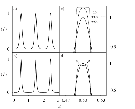
Figure 3: Plot of the average current as a function of the magnetic flux $\varphi$ for a) $g=\nu=1$, b) $g=\nu=1/3$ at $k_{\rm B}T=0.1E_{\rm c}$. A zoom on the shape of the resonance peak is plotted for c) $g=\nu=1$ and d) $g=\nu=1/3$ with different temperatures $k_{\rm B}T=0.01,0.005,0.001E_{\rm c}$. Other parameters: $e^{*}V=0.05E_{\rm c}$, $\eta=1$. Curves in panels a) and b) are normalized to the on-resonance value, while curves in panels c) and d) are normalized to the maximum value of the current at $k_{\rm B}T=0.01E_{\rm c}$ (solid line).

IV Results

This Section is organized as follows: we describe current, Fano factor and skewness assuming $g=\tilde{g}$, and we discuss various limits in the temperature, voltage and flux range, referring to the diamonds in Fig. 2c).

IV.1 Current

A great deal of information on the interaction parameter can be gathered from the analysis of the DC current, although it is not possible to extract signatures of the fractional charge. In this subsection we consider $g=\nu$, despite the generalization $g\neq\nu$ is straightforward.

IV.1.1 Magnetic flux dependence

In the low-voltage regime $e^{*}V\lesssim 2E_{\rm c}$ (diamonds I and II in Fig. 2c)) a simple analytical form for the current can be found; here, only two adjacent antidot charge states are connected through open rates and charge transport takes place in a sequence of $n\to n+1\to n$ processes.

In regions I transport is exponentially suppressed because of the finite energy $E_{\rm c}$; in regions I,II current at fixed source-drain voltage oscillates as a function of $\varphi$ with a periodicity of one flux quantum $\Phi_{0}$ for any $\nu$ and $g$, in accordance with gauge invariance.byeryang This is represented in Fig. 3a) and b) obtained from a numerical solution of the master equation.

Because of periodicity in $\varphi$, we start at $n=0$. The current is

$$\langle I\rangle=\eta|e^{*}||t_{L}|^{2}\frac{\Gamma_{+}^{0}\Gamma_{-}^{0}f_{-}(e^{*}V)}{\Gamma_{\rm tot}},$$ (26)

where

$$\Gamma_{\rm tot} = \Gamma_{+}^{0}f_{+}(E_{+}^{0})+\eta\Gamma_{-}^{0}f_{+}(E_{-}^{0}),$$

$$f_{\pm}(x) = 1\pm e^{-\beta x}.$$ (27)

If temperature is lowered until $k_{\rm B}T\ll e^{*}V$, then a qualitative difference appears in the shape of the resonance peaks as a function of $g$. When $g<1$, due to the non-monotonic rates the current develops two side peaks across the resonance and develops a minimum on resonance (Fig. 3d)). On the other hand, for $g=1$ the rates Eq. (19) are Fermi functions and the current peak displays no structure regardless of the ratio $e^{*}V/k_{\rm B}T$. The only effect is that for lower $T$ plateaus appear with increasing width (Fig. 3c)).

It is worth mentioning that the double-peak structure for $g<1$ was already established in resonant qp tunneling through localised impurities,chamon although in our case the parameter that tunes the resonance is the magnetic flux.

If bias voltage is increased, one enters regimes where more charge states participate to transport. For voltages $2E_{\rm c}<e^{*}V<4E_{\rm c}$ one needs to consider two or three charge states. As an example of regions III, we discuss the diamond where the rates $\Gamma^{p}_{\pm},\overline{\Gamma}_{\pm}^{p}$, $p=n,n+1$, are open to transport and the states with $n,n+1$ and $n+2$ qp are involved. Again, periodicity allows to choose the starting point $n=0$. Furthermore, in our temperature regime only two backward rates can be retained, $\overline{\Gamma}_{-}^{0}$ and $\overline{\Gamma}_{+}^{1}$ (Fig. 4, left panel). One finds:

$$\langle I\rangle=\eta|e^{*}||t_{L}|^{2}\frac{\Gamma_{+}^{1}\Gamma_{-}^{1}\Gamma_{t}^{0}+\Gamma_{+}^{0}\Gamma_{-}^{0}\Gamma_{t}^{1}}{\Gamma_{t}^{0}(\Gamma_{+}^{1}+\Gamma_{t}^{1})+\eta\Gamma_{-}^{0}\Gamma_{t}^{1}},$$ (28)

where $\Gamma^{0}_{t}=\Gamma_{+}^{0}+\eta\overline{\Gamma}_{-}^{0}$ and $\Gamma^{1}_{t}=\eta\Gamma_{-}^{1}+\overline{\Gamma}_{+}^{1}$. Here also double-peak structures appear at fixed bias voltage as a function $\varphi$, although they have a more complicated behaviour. Indeed, close to the diamond onset, $e^{*}V\approx 2E_{\rm c}$, the current for $g<1$ develops a broad minimum around $\varphi=1$ for large temperature, then a maximum in an intermediate range, and finally a minimum again with sharp side-peaks at $\beta E_{\rm c}\gg 1$ (Fig. 4, right panel b)). No structure appears for $g=1$, where decreasing the temperature has the only effect of shrinking the peak width and causing a larger plateau (Fig. 4, right panel a)).

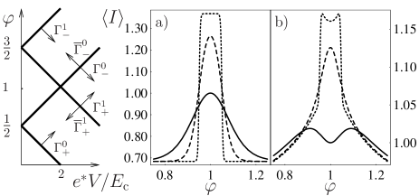
Figure 4: Left panel: scheme of the retained rates in the approximation for the three-state region. Right panel: a) current versus $\varphi$ at $g=\nu=1$ for $\beta E_{\rm c}=10,25,200$, with solid, dashed, dotted curves respectively. The curves are at fixed $e^{*}V/E_{\rm c}=2.2$ and $\eta=1$, and are normalized to the value of the lowest temperature curve at $\varphi=1$. b) the same with $g=\nu=1/3$.

IV.1.2 Bias voltage dependence

A plot of the current is presented in Fig. 5 as a function of the source-drain voltage for symmetric barriers. Again the rate behaviour for $g=1$ or $g<1$ changes qualitatively the current. While for $g=1$ the current reflects the Fermi-liquid nature of the leads and increases in steps, non-monotonic features appear for $g=1/3$ and lead to negative differential conductance (Fig. 5 b)). Two features are most remarkable in this sense: the on-resonance peak (curve at $\varphi=0.5$) for small voltage and the off-resonance peak (curve at $\varphi=0$) at $e^{*}V\approx 6E_{\rm c}$, indicated with arrows in Fig. 5 b).

Figure 5: Current as a function of voltage for $g=\nu=1$ (top) and $g=\nu=1/3$ (bottom). The lines correspond to $\varphi=0,0.2,0.5$ and are shifted of $0.0015I_{0}$ ($0.15I_{0}$) with respect to the curve at $\varphi=0$. Other parameters are $\eta=1$ and $k_{\rm B}T=0.1E_{\rm c}$. Current units are $I_{0}=|e^{*}|\omega_{c}|t_{L}|^{2}(\beta\omega_{c})^{1-g}(2\pi)^{g-3}/\mathbf{\Gamma}(g)$.

The first peak develops in region II and can be described with Eq. (26). Setting $\varphi=1/2$ and $\eta=1$, one finds

$$\langle I\rangle=|e^{*}||t_{L}|^{2}\frac{\Gamma^{0}_{+}}{2}f_{-}\left(\frac{e^{*}V}{2}\right).$$ (29)

This result allows for a determination of the Luttinger parameter $g$ from the power-law behaviour of the rate, $\Gamma^{0}_{+}\propto\left(\beta e^{*}V/4\pi\right)^{g-1}$, valid for $\beta e^{*}V\gg 1$.

The second feature finds a natural explanation in terms of antidot plasmonic excitations. These in fact enter into play for $e^{*}V>\epsilon=2E_{\rm c}/\nu$. This new mode increases non-monotonically the tunneling rate, leading to peaks in current.

To ascribe the onset of the peak to plasmons, we focus on the above example with $g=\nu=1/3$ and $\epsilon=2E_{\rm c}/\nu=6E_{\rm c}$. Here, one has to consider five charge states, $n,\ldots,n+4$ and the rates $\Gamma^{p}_{\pm}$, $p=n,\ldots,n+3$. In this regime it is possible to obtain an approximate form of the current neglecting all backward rates except those opening at the border of region V ($\overline{\Gamma}^{0}_{-},\overline{\Gamma}^{3}_{+}$, see Fig. 6, inset). We work at $\varphi=2$, choosing $n=0$ as a reference. Observing that the large-energy behaviour of the forward rates is $\propto(\beta E)^{g-1}$, we can process the rates according to the magnitude of their argument in region V: furthermore, for $\eta=1$, $\Gamma_{+}^{l}=\Gamma_{-}^{3-l}$ with $l=0,1,2,3$. Thus we set $\Gamma_{\pm}^{1}=\Gamma_{\pm}^{2}\sim f$, with $f$ a temperature dependent constant, since these rates are in their slow-decaying regime. On the opposite, the full energy dependence of $\Gamma^{3}_{+}=\Gamma^{0}_{-}$ is taken into account. In terms of the ’plus’ rates only, the current is given by

$$\langle I\rangle=2|e^{*}|\frac{f\,\overline{\Gamma}_{+}^{3}+\Gamma^{0}_{+}\left(\Gamma^{3}_{+}+f\right)}{3\Gamma^{0}_{+}+2\Gamma_{+}^{3}+3\overline{\Gamma}^{3}_{+}}.$$ (30)

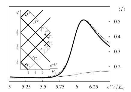
Figure 6: Current in the IV-V state regime versus bias voltage at $g=\nu=1/3$. Solid line, numerical result; dot-dashed line, approximate solution in Eq. (30) with $\delta\Gamma_{p}=g\Gamma^{3}_{+}$; dashed line, approximate solution without plasmons ($\delta\Gamma_{p}=0$). The curves are at $\varphi=2$ (equivalent to $\varphi=0$ in Fig. 5 because of the periodicity in magnetic flux), $k_{\rm B}T=0.1E_{\rm c}$, $\eta=1$ and units are as in Fig. 5. The best fit parameter is $f=0.19I_{0}/|e^{*}|$. Inset: scheme of retained rates in the approximation for region V.

Finally, we set $\Gamma^{0}_{+}\sim f+\delta\Gamma_{p}$, where $\delta\Gamma_{p}$ is the first plasmon contribution to the rate that shows up as a secondary peak at energy $E=\epsilon$. We now compare the current with no plasmons ($\delta\Gamma_{p}=0$) with $\delta\Gamma_{p}=g\Gamma^{3}_{+}$ obtained from Eqs. (18) and (20) with relative weight $w_{1}/w_{0}=\mathbf{\Gamma}(g+1)/\mathbf{\Gamma}(g)=g$ . Figure 6 shows a comparison between the current with these approximations and the result obtained through a numerical solution of the master equation. It is apparent that neglecting the plasmon completely misses the peak onset that is instead well-captured by out latter approximation. This testifies that plasmonic excitations play indeed the crucial role in current enhancement.

IV.2 Current moments

Current moments are now discussed.merlo According to Eq. (22), these two quantities are the natural observables to look at in order to measure the quasiparticle charge $e^{*}$. In the antidot geometry, different conditions can be found where this measurement is special in the sense discussed above. We remind that for a poissonian process, as with weak backscattering current in a point contact, $k_{2}=e^{*}/e=\nu$, $k_{3}=(e^{*}/e)^{2}$.

IV.2.1 Few-state regime: $e^{*}V\lesssim 2E_{\rm c}$

For the sequential tunneling master equation Eq. (23) restricted to the two-state regime (two charge states), an exact analytical treatment is possible.

A known formulaBlanterReview ; braggio for the Fano factor is obtained

$$k_{2}=\left(\frac{e^{*}}{e}\right)\left(\coth\left(\frac{\beta e^{*}V}{2}\right)-2\eta\frac{\Gamma_{+}^{0}\Gamma_{-}^{0}f_{-}(e^{*}V)}{\Gamma_{\rm tot}^{2}}\right),$$ (31)

while for the skewness we find

$$k_{3} = \left(\frac{e^{*}}{e}\right)^{2}\bigg{(}1-6\eta\frac{\Gamma_{+}^{0}\Gamma_{-}^{0}f_{+}(e^{*}V)}{\Gamma_{\rm tot}^{2}}+$$ (32)

$$\qquad\qquad+12\eta^{2}\frac{{\Gamma_{+}^{0}}^{2}{\Gamma_{-}^{0}}^{2}f_{-}^{2}(e^{*}V)}{\Gamma_{\rm tot}^{4}}\bigg{)},$$

with the functions $\Gamma_{\rm tot},f_{\pm}$ defined in Eq. (IV.1.1). The previous equations are an example of the intertwining between charge and process statistics that does not allow, in general, for unequivocal conclusions on $e^{*}$. We analyse now the behaviour varying the ratio $e^{*}V/k_{\rm B}T$ looking for special conditions.
Thermal limit: $e^{*}V\ll k_{\rm B}T$. The Fano factor is independent of the charge fractionalization,

$$k_{2}=2\frac{k_{\rm B}T}{eV},$$ (33)

reflecting the fluctuation-dissipation theorem. On the contrary, the normalized skewness that measures the fluctuation asymmetry induced by the current depends on the carrier charge $e^{*}=\nu e$. Indeed, for low voltages $V\to 0^{+}$ one has

$$k_{3}=\left(\frac{e^{*}}{e}\right)^{2}\left[1-3\frac{\eta}{(1+\eta)^{2}}\frac{1}{{\rm Cosh}^{2}(\beta E_{\rm c}(\varphi-1/2))}\right].$$ (34)

Note that the $\varphi$ dependence can be used to extract $\eta$ and $e^{*}/e$ independently from $g$.
Shot limit: $k_{\rm B}T\ll e^{*}V$. In the blockade regions I with $|\beta E_{\pm}^{0}|\gg 1$, one has $k_{2}=\nu$ and $k_{3}=\nu^{2}$. In this case the statistics of the transport process is poissonian: the transport through the antidot is almost completely suppressed, $\langle I\rangle\approx 0$, and the residual current is generated only by a thermally activated tunneling that is completely uncorrelated. So regions I constitute an example of special regime.

Figure 7: Fano factor (left) and skewness (right) as a function of $\varphi$. Panels a) and b) $\eta=1$, panels c) and d) $\eta=3$. Parameters: $e^{*}V=0.1E_{\rm c}$, $k_{\rm B}T=0.004E_{\rm c}$ and $g=1/5$ (solid line), $g=1/3$ (dot-dashed line), $g=1/2$ (dotted line). Horizontal thin lines indicate the universal limits at 1/2 at 1/4.

We consider now the two-state regime (II) for $\beta E_{\pm}^{0}\gg 1$. For fractional edges $g<1$, $k_{2,3}$ have a particular functional dependence on $\varphi$. We find that they both develop a minimum and that for not too strong asymmetries the absolute values of the minima are

$$k_{n}^{\rm min} = \frac{\nu^{n-1}}{2^{n-1}}.$$ (35)

These minimal values do not depend neither on $g$, as the comparison of solid ($g=1/5$), dotted ($g=1/3$) and dashed ($g=1/2$) curves in Fig. 7 confirms, nor on $\eta$. For Fermi liquid edges $g=1$, we have

$$k_{2} = \nu(1+\eta^{2})/(1+\eta)^{2}$$

$$k_{3} = \nu^{2}\left[1-6\eta(1+\eta^{2})/(1+\eta)^{4}\right],$$ (36)

independently from $\varphi$. Here, $k_{2}$ and $k_{3}$ assume their minimal values $\nu/2$ and $\nu^{2}/4$ in the symmetric case $\eta=1$. In this conditions we have the strongest anticorrelation that is signalled by a marked sub-poissonian statistics.

We can conclude that in the two-state regime, in the shot limit, the values of the minima for $k_{2,3}$ obtained varying $\eta,\varphi$ correspond to a special condition where the system shows the same universal sub-poissonian statistics for any $g\leq 1$. This represents a means of testing fractional charge outside poissonian conditions and insensitive to renormalizations of the Luttinger parameter.

In the intermediate regime $e^{*}V\approx k_{\rm B}T$, $k_{2,3}$ depend more strongly on the parameter $g$, and the interplay of these two energy scales prevents the onset of special regimes.

IV.2.2 Many-state regime: $e^{*}V>2E_{\rm c}$

We study now higher voltages $e^{*}V>2E_{\rm c}$ where the renormalized interaction parameter $g$ has a prominent role. For this purpose we consider the behaviour of both the Fano factor and the normalized skewness. In Fig. 8 a density plot of $k_{2}$ and $k_{3}$ for $\nu=g=1/3$ as a function of magnetic flux and source-drain voltage is shown for different asymmetries.

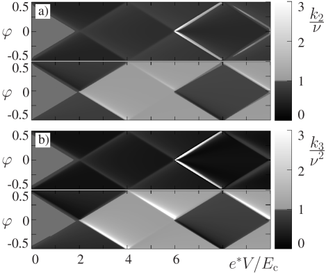
Figure 8: Panel a): Fano factor $k_{2}/\nu$ at $\nu=g=1/3$, $k_{\rm B}T=0.02E_{\rm c}$, vs. source-drain voltage and $\varphi$. Panel b): normalized skewness $k_{3}/\nu^{2}$ with the same parameters. Both moments are plotted for symmetric barriers $\eta=1$ (top) and strong asymmetry $\eta=10$ (bottom).

First of all, in region I we recover poissonian statistics: $k_{2}=\nu$, $k_{3}=\nu^{2}$ (middle grey) for any $\eta$. Outside this region, light grey zones represent super-poissonian Fano factor and normalized skewness ($k_{2}>\nu$ and $k_{3}>\nu^{2}$), while dark grey regions represent sub-poissonian behaviour ($k_{2}<\nu$ and $k_{3}<\nu^{2}$). Figure 8 shows that super-poissonian regions are possible with $g<1$. For $g\geq 1$, we always have sub-poissonian behaviour in accordance with previous results (not shown).braggio In presence of asymmetry, super-poissonian regions increase. We note that Fano and skewness present concurrent super/sub-poissonian behaviour, and that the maximal values of the skewness in the super-poissonian regions are stronger. Given this similarity, in the following we will discuss the Fano factor only.
Three-state region. In region III, a tractable analytical formula for the Fano factor can be derived under the same assumptions made for the current Eq. (28): one has $k_{2}/\nu=1-2\eta\,\,\delta k_{2}$, with

$$\delta k_{2}\!=\!\frac{{\Gamma^{0}_{t}}^{2}\Gamma_{+}^{1}\Gamma_{-}^{1}\!+\!{\Gamma^{1}_{t}}^{2}\Gamma_{+}^{0}\Gamma_{-}^{0}\!+\!\Gamma_{-}^{0}\Gamma_{+}^{1}\left(\Gamma^{0}_{t}\!-\!\Gamma^{1}_{t}\right)\left(\eta\Gamma_{-}^{1}\!-\!\Gamma_{+}^{0}\right)}{\left[\eta\Gamma_{-}^{0}\Gamma_{t}^{1}+\Gamma_{t}^{0}\left(\Gamma_{+}^{1}+\Gamma_{t}^{1}\right)\right]^{2}},$$ (37)

with $\Gamma^{0}_{t},\Gamma^{1}_{t}$ in Eq. (28). We note that in order to have super-poissonian noise a fractional $g<1$ is necessary, with additional conditions on the asymmetry. Indeed, setting $\eta=1$ in Eq. (37) in the limit $\beta E_{+}^{1},\beta E_{-}^{0}\gg 1$ yields $\delta k_{2}>0$ for any $g$. On the other side, setting $g=1$ gives $\delta k_{2}=2\eta/(\eta^{2}+\eta+1)^{2}>0$. It appears that positive correlations are induced by an interplay of $\eta$ and $g$.
Five-state region. Finally, interesting effects take place in the five-state regime (V) for $\nu=1/3$. Here, a strongly super-poissonian Fano factor appears along the diamond lines for $\eta=1$ and disappears for large asymmetries. An investigation of this effect can be performed with the same methods used to obtain Fig. 6. The rate enhancement due to the onset of the plasmonic collective excitations can again be shown to be responsible of the super-poissonian behaviour at small asymmetries.

V Conclusions

In conclusion, we have analysed transport of quasiparticles through an antidot coupled with edge states in the fractional Hall regime. The model of a finite size chiral Luttinger liquid with periodic boundary conditions has been reviewed and cast in a suitable form for calculations of higher current moments through a master equation approach in the sequential regime. We have also allowed for the possibility of a phenomenological renormalization of the interaction parameter.

We have found that independent information on interaction renormalization and fractional charge can be extracted from tunneling current and its moments, noise and skewness. For current, remarkable qualitative differences as a function of the Luttinger parameter appear in the shot limit of resonance peaks and in the three-state regime. A quantitative determination of $g$ is furthermore possible through the power-law behaviour of on-resonance current versus voltage at low temperatures. Current moments also depend strongly on the interaction parameter: in particular, super-poissonian behaviour is never found for $g\geq 1$ regardless of asymmetry. On the other hand, we have identified special regimes in the one- and two-state regions where a comparison of Fano factor and normalized skewness realizes an unambiguous charge determination procedure, insensitive to renormalizations of $g$. Finally, signatures of plasmonic excitations are indicated in the large bias voltage regime.

Confirmation of such novel results appears to be within reach: plugging estimated parameters from present experimentsgold into our results gives currents in the range of $0.5\div 5$ pA for $g=1/3$ and $T=10$ mK. At the same time, recent accomplishments in measurement techniques applied to electron counting open the possibility for feasible noise and skewness determination, even in systems with very low current and noise levels.skewness

Furthermore, litographic approaches have been developed that allow for antidot radii sensibly smaller than the 300 nm in the original experiments.goldpriv Thus, the energy scale $E_{\rm c}$ associated with the antidot finite size can be raised to the order of some hundreds of mK, and more easily attainable temperature regimes can be compatible with the requirements of our approximations.

We believe that our results help clarify some issues related to transport in the Hall regime, namely features like fractional charges and nonpoissonian correlations. Such a thorough analysis of a Hall antidot device is a necessary building block, especially in view of possible applications of similar systems to topological quantum computation.averin

We thank E. Fradkin, M. Heiblum, V. Pellegrini, J. Jain, V. Goldman, and M. Governale for useful discussions. We acknowledge partial support from ESF activity INSTANS. Financial support by the EU via Contract No. MCRTN-CT2003-504574 and by the Italian MIUR via PRIN05 is gratefully acknowledged.

References

- (1) R. B. Laughlin, Phys. Rev. Lett. 50, 1395 (1983).
- (2) B. I. Halperin, Phys. Rev. Lett. 52, 1583 (1984); D. Arovas, J. R. Schrieffer, and F. Wilczek, ibid. 53, 722 (1984).
- (3) X. G. Wen, Phys. Rev. Lett. 64, 2206 (1990); Phys. Rev. B 41, 12838 (1990); 43, 11025 (1991).
- (4) C. L. Kane and M. P. A. Fisher, Phys. Rev. Lett. 72, 724 (1994).
- (5) R. de-Picciotto, M. Reznikov, M. Heiblum, V. Umansky, G. Bunin, and D. Mahalu, Nature (London) 389, 162 (1997); L. Saminadayar, D. C. Glattli, Y. Jin, and B. Etienne, Phys. Rev. Lett. 79, 2526 (1997).
- (6) A. M. Chang, L. N. Pfeiffer, and K. W. West, Phys. Rev. Lett. 77, 2538 (1996); M. Grayson, D. C. Tsui, L. N. Pfeiffer, K. W. West, and A. M. Chang, ibid. 80, 1062 (1998).
- (7) Y. C. Chung, M. Heiblum, and V. Umansky, Phys. Rev. Lett. 91, 216804 (2003).
- (8) S. Roddaro, V. Pellegrini, F. Beltram, G. Biasiol, and L. Sorba, Phys. Rev. Lett. 93, 046801 (2004).
- (9) U. Zülicke, J. J. Palacios, and A. H. MacDonald, Phys. Rev. B 67, 045303 (2003).
- (10) E. V. Tsiper and V. J. Goldman, Phys. Rev. B 64, 165311 (2001).
- (11) V. J. Goldman and E. V. Tsiper, Phys. Rev. Lett. 86, 5841 (2001).
- (12) A. Boyarsky, V. V. Cheianov, and O. Ruchayskiy, Phys. Rev. B 70, 235309 (2004).
- (13) S. S. Mandal and J. K. Jain, Phys. Rev. Lett. 89, 096801 (2002).
- (14) B. Rosenow and B. I. Halperin, Phys. Rev. Lett. 88, 096404 (2002).
- (15) O. Heinonen and S. Eggert, Phys. Rev. Lett. 77, 358 (1996).
- (16) S. Khlebnikov, Phys. Rev. B 73, 045331 (2006).
- (17) L. S. Levitov, A. V. Shytov, and B. I. Halperin, Phys. Rev. B 64, 075322 (2003).
- (18) E. Papa and A. H. MacDonald, Phys. Rev. Lett. 93, 126801 (2004); Phys. Rev. B 72, 045324 (2005).
- (19) X. Wan, F. Evers, and E. H. Rezayi, Phys. Rev. Lett. 94, 166804 (2005).
- (20) K. Yang, Phys. Rev. Lett. 91, 036802 (2003).
- (21) X. Wan, E. H. Rezayi, and K. Yang, Phys. Rev. B 68, 125307 (2003).
- (22) Y. N. Joglekar, H. K. Nguyen, and G. Murthy, Phys. Rev. B 68, 035332 (2003).
- (23) E. Papa and T. Stroh, Phys. Rev. Lett. 97, 046801 (2006); Phys. Rev. B 75, 045342 (2007).
- (24) M. R. Geller and D. Loss, Phys. Rev. B 56, 9692 (1997).
- (25) A. Braggio, N. Magnoli, M. Merlo, and M. Sassetti Phys. Rev. B 74, 041304(R) (2006).
- (26) V. J. Goldman, J. Liu, and A. Zaslavsky, Phys. Rev. B 71, 153303 (2005); V. J. Goldman, I. Karakurt, Jun Liu, and A. Zaslavsky, ibid. 64, 085319 (2001).
- (27) M. Kataoka, C. J. B. Ford, G. Faini, D. Mailly, M. Y. Simmons, D. R. Mace, C.-T. Liang, and D. A. Ritchie, Phys. Rev. Lett. 83, 160 (1999); M. Kataoka, C. J. B. Ford, M. Y. Simmons, and D. A. Ritchie, ibid. 89, 226803 (2002).
- (28) T. G. Griffiths, E. Comforti, M. Heiblum, A. Stern, and V. Umansky, Phys. Rev. Lett. 85, 3918 (2000).
- (29) C. L. Kane and M. P. A. Fisher, Phys. Rev. B 46, 15233 (1992).
- (30) This fact was observed in the paper of Griffiths et al. (Ref. griffiths, ).
- (31) H. Saleur and U. Weiss, Phys. Rev. B 63, 201302(R) (2001); A. Komnik and H. Saleur, Phys. Rev. Lett. 96, 216406 (2006).
- (32) S. Kettemann, Phys. Rev. B 55, 2512 (1997).
- (33) E. Fradkin, in Proceedings of the XXXIV Rencontres De Moriond, Les Arcs, France, EDP Sciences (1999).
- (34) M. R. Geller and D. Loss, Phys. Rev. B 62, R16298 (2000).
- (35) This does not mean that a localized flux is actually needed in experiments. Such a modelization simply takes into account the fact that the infinite edges are insensitive to the strength of the external magnetic field as long as incompressibility is present. Indeed, in real experiments the antidot flux is changed sweeping the external magnetic field, as in Ref.gold, .
- (36) A. Furusaki, Phys. Rev. B 57, 7141 (1998).
- (37) A. Braggio, M. Grifoni, M. Sassetti, and F. Napoli, Europhys. Lett. 50, 236 (2000).
- (38) A. Braggio, R. Fazio, and M. Sassetti, Phys. Rev. B 67, 233308 (2003).
- (39) S. Eggert, A. E. Mattsson, and J. M. Kinaret, Phys. Rev. B 56, R15537 (1997).
- (40) L. S. Levitov and M. Reznikov, Phys. Rev. B 70, 115305 (2004).
- (41) D. A. Bagrets and Yu. V. Nazarov, Phys. Rev. B 67, 085316 (2003).
- (42) N. Byers and C. N. Yang, Phys. Rev. Lett. 7, 46 (1961).
- (43) C. de C. Chamon and X. G. Wen, Phys. Rev. Lett. 70, 2605 (1993).
- (44) Y. M. Blanter and M. Büttiker, Phys. Rep. 336, 1 (2000).
- (45) Yu. Bomze, G. Gershon, D. Shovkun, L. S. Levitov, and M. Reznikov, Phys. Rev. Lett. 95, 176601 (2005); S. Gustavsson, R. Leturcq, B. Simovic, R. Schleser, T. Ihn, P. Studerus, K. Ensslin, D. C. Driscoll, and A. C. Gossard, ibid. 96, 076605 (2006).
- (46) V. J. Goldman, private communication.
- (47) D. V. Averin and V. J. Goldman, Solid State Comm. 121, 25 (2001).