On the theory of Bose Einstein condensation of quasiparticles: on the possibility of condensation of ferromagnons at high temperatures

Abstract

The Bose condensation of magnons in physical systems of finite size is considered for the case of ferromagnetic thin films. It is shown that in accordance with present-day experimental capabilities, which permit one to achieve densities of long-wavelength spin excitations of $\sim 10^{18}$–$10^{19}$ ^-3, in such films, the formation of a coherent condensate of such quasiparticles begins at temperatures $T\sim 10^{2}$K (including room temperature). It is found that Bose condensation is accompanied by a scaling phenomenon, according to which the main thermodynamic variable is not the number of particles $N$ but the ratio $N/T$. This indicates that the Bose condensation of magnons can be observed at relatively low magnon densities (and, accordingly, low pumping). The roles played by the shape of the spectrum of spin excitations and by the film thickness for observation of the phase transition to the state with the Bose condensate are analyzed, and the partial contributions of dierent groups of quasiparticles to the total spectral distribution of magnons over energies are discussed.

PACS: 05.30.Jp, 75.30.Ds, 75.70-i

KEYWORDS: Bose condensation, magnons, spectral density, phase transition

1 Introduction

The Bose Einstein condensation (BEC) of atoms and molecules [1, 2] has become one of the most remarkable phenomena that reveal and confirm the quantum nature of a number of macroscopic processes. The formation of a Bose condensate, i.e., the accumulation of identical particles with integer spin in one of the quantum states, may be inherent both to true particles (atoms, molecules) and to quasiparticle excitations of multiparticle systems. In this sense, quasiparticles — excitons and biexcitons and also magnons are of particular interest, since, existing only as excited states, they are actually absent (if one ignores the thermal background) in systems at normal temperature and pressure. Ordinarily, except under specially chosen conditions, the equilibrium density of thermal quasiparticles decreases with decreasing temperature. Therefore, the study of BEC of quasiparticles, or their “nonthermal” accumulation in one of the states, requires, first and foremost, the presence of a macroscopic (essentially nonequilibrium) total number of quasiparticles. This can be achieved only by using methods of creating and maintaining a large number of quasiparticles in condensed systems, at least for a time sufficient for, first, their relatively rapid thermalization and, second, subsequent BEC. Under such conditions the latter will occur as a (quasi-)equilibrium phenomenon at a conserved (on average) number of quasiparticles, which is ensured by some external source of intense quasiparticle creation.

BEC is a phenomenon associated, as a rule, with very low temperatures: the critical temperature $T_{\rm BEC}$ at which a Bose condensate is created depends on the gas density $\mathfrak{n}$ and the mass $m$ of its constituent particles according to the well-known formula [3]

$$T_{\rm BEC}=\frac{{\mathfrak{n}}^{2/3}}{m}\frac{2\pi\hbar^{2}}{k_{B}\zeta^{2/3}(3/2)}\,\,,$$ (1.1)

where $\zeta(x)$ is the Riemann $\zeta$-function. For example, in experiments on the observation of BEC [4, 5] because of the large mass of the atoms of alkali elements and low density (approximately $10^{3}$ particles in a volume of $\sim 10^{-6}\ {\text{ }}^{3}$) the system must be “cooled” down to $10^{-9}\ldots 10^{-8}$K. Or, for example, in the case of the “most ideal‘’ of the real gases, helium, the temperature of the transition to the Bose-condensed state has a value $T_{\rm BEC}\approx 2\times 10^{-2}$ at a density $\approx 10^{19}{\text{ }}^{-3}$, which corresponds to a gaseous state. It is therefore obvious that observation of BEC at high (up to room) temperatures is possible only in systems consisting of light (weakly interacting) bosons. As has been mentioned repeatedly, quasiparticle excitations, the effective mass of which is rather small — in particular, comparable to the electron mass $m_{e}$ — are well suited to the role of such bosons.

In the discussion of the BEC of quasiparticles, attention has apparently been focused primarily on excitons and biexcitons. Starting with the pioneering work of Moskalenko [6] and Keldysh [7], many papers have been devoted to the study of the phase diagram of semiconductors at high densities of nonequilibrium electrons and holes and also to attempts to observe different types of their joint condensed states. Despite the short lifetime of excitonic states and the intense processes of electron hole annihilation, there have been several pieces of convincing experimental evidence in favor of the observation of exciton (and biexciton) BEC [8].

However, there are other promising systems for studying the BEC of quasiparticles. In particular, among the interesting objects suitable for this (see Ref. [9]) are magnets, including ferromagnetic insulators, where high densities of magnons (up to $10^{18}$–$10^{19}{\text{ }}^{-3}$) can be created by pulsed microwave pumping. We recall that magnons, which are elementary excitations above the magnetization field, to good approximation obey Bose statistics Their spectrum is formed on account of the presence of several interactions, chief among which are the exchange and magnetic dipole dipole interactions [10]. The first of these determines an isotropic spectrum of spins waves with wavelengths $k^{-1}$, less than the characteristic size $L$ of the system, so that $kL\gg 1$. The second, on the contrary, operates at wavelengths for which $kL\leq 1$ and, furthermore, leads to dependence of the magnon spectrum on the direction of $\mathbf{k}$. Analysis of the conditions for BEC of specifically these elementary excitations in comparatively thin slabs (microfilms) is the subject of the present study, which is directed toward the task of examining the conditions for observation and the features of BEC in ferromagnetic insulating films with different shapes of the spin-wave spectrum. We consider magnons to be very promising for research on the BEC of quasiparticles for at least several reasons. First, they have a relatively long lifetime and, as we have said, can have densities reaching $\sim 10^{19}{\text{ }}^{-3}$; second, there are technologies in place for growing very thin (less than $\lesssim 10\,\mu m$ thick) films with rather perfect structure and for making precision measurements of the magnon spectrum in them by optical methods; third, the temperature and magnetic field can be easily varied over wide limits, permitting detailed comparison of theory and experiment.

We note that in recent years a rather large number of papers have appeared (e.g., Refs. [11]–[16]) in which the idea of BEC of magnons has been used for describing phase transitions in (predominantly) antiferromagnets from their nonmagnetic (singlet) state to a magnetically ordered state under the influence of an external magnetic field. The point is that the induced appearance of magnetization in finite fields can actually be formally described and interpreted in the language of condensation of magnetic excitations. However, BEC as such does not occur, since there one is talking about only a rearrangement of the ground state of the system and, consequently, of virtual and not real magnons (see, e.g., Ref. [17]). In contrast, the focus of our attention here is on real — excited — states that appear as a consequence of pumping electromagnetic energy into the system, this energy going to the creation of quasiparticles above the ground state, as was masterfully done in a recent experimental study with the use of microfilms of yttrium iron garnet (YIG) [18].

2 Model and general relations

Suppose that we have a ferromagnetic crystal in the form a parallelepiped (see Fig. 1) of volume $V=L_{x}L_{y}L_{z}$.

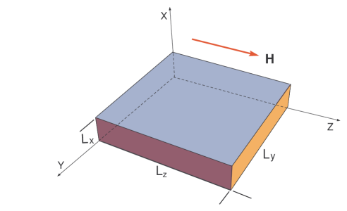
Figure 1: Shape of the ferromagnetic crystal.

The number of sites $N_{j}$ along the corresponding axes ($j$ takes the values $x,\ y,\ z$) is determined by the lattice parameters $a_{j}$: $N_{j}=L_{j}/a_{j}+1$. As we know, the magnetic ground state of such a crystal presupposes an identical direction of all the spins (e.g., along the quantization axis $z$), while the lowest excited state corresponds to one “flipped” spin [19, 20]. From a linear combination of such states one can construct an eigenstate in the form a spin wave with amplitude $b_{\mathbf{q}}(\mathbf{r})$. The form of these amplitudes depends on the boundary conditions. Usually for simplification one uses cyclic boundary conditions, when the amplitudes are identical at opposite faces of the crystal. Then the amplitudes have the form of a plane wave:

$$b_{\mathbf{q}}(\mathbf{r})=\exp(i\mathbf{q}\mathbf{r})\,\prod_{j}N_{j}^{-1/2}\,,$$ (2.1)

where in the given case the vector $\mathbf{r}$ enumerates lattice sites — $r_{j}=1,\,2,\,\ldots,\,N_{j}$, and the dimensionless quasimomentum $\mathbf{q}$ is defined in the Brillouin zone $(-\pi<q_{j}\leq\pi)$ and takes on a discrete spectrum of values with a step $\Delta q_{j}^{per}=2\pi/N_{j}$.

If, on the contrary, the spins on the faces are “free”, the solution of the boundary condition problem with the corresponding (free) boundary conditions leads to amplitudes that differ from (2.1):

$$b_{\mathbf{q}}(\mathbf{r})=\prod_{j}\sin(q_{j}r_{j})[2/(N_{j}+1)]^{1/2}\,.$$ (2.2)

The Brillouin zone here is defined somewhat differently: $0<q_{j}<\pi$, and the discreteness step is $\Delta q_{j}^{free}=\pi/(N_{j}+1)$. Let us point out the main differences between the quasimomentum spectra in (2.1) and (2.2). First, for periodic boundary conditions there exists a zero mode $\mathbf{q}=0$, while for the free boundary conditions there is not: the minimum value that can be taken on by each of the quasimomentum components is $q_{j}^{min}=\Delta q_{j}^{free}$. Second, the quasimomentum spectrum for free boundary conditions is twice as dense as for periodic boundary conditions, since for $N_{j}\gg 1$ the ratio $\Delta q_{j}^{per}/\Delta q_{j}^{free}=2N_{j}/(N_{j}+1)\approx 2$.

It is considered to be almost obvious that the concrete form of the boundary conditions does not influence the behavior of physical quantities. Actually this is true if one is talking about very “large” systems. However, as will be shown below, for “small” systems the difference mentioned above — the absence of a zero mode in the spectrum for the case of free boundary conditions — leads to quite perceptible contributions (Weyl corrections) to certain observable characteristics which are absent in the case of idealized periodic boundary conditions. Since we intend to investigate the question of BEC in microfilms $\sim 1\mu m$ thick, the use of free boundary conditions is justified as more realistic.

In spite of the differences indicated, the expression for the magnon energy due to the isotropic exchange interaction is the same for both kinds of boundary conditions and can be written in dimensionless form as

$$\epsilon(\mathbf{q})=2\sum_{j}\sin^{2}\frac{q_{j}}{2}\,.$$ (2.3)

Far from the Brillouin zone boundary or in long-wavelength region $(q_{j}\ll\pi)$, it follows from (2.3)) that

$$\epsilon(\mathbf{q})=\frac{\mathbf{q}^{2}}{2}\,.$$ (2.4)

The dimensional quantities are easily restored through the dimensions of the crystal $L_{j}$, the lattice parameters $a_{j}$, and the effective mass $m_{m}$, which for magnons is inversely proportional to the exchange integral. Then the components of the quasimomentum for the case of free boundary conditions

$$p_{j}=\hbar\,\frac{q_{j}}{a_{j}}\approx\hbar\pi\frac{k_{j}}{L_{j}},\quad k_{j}=1,2,\ldots,N_{j},$$

while the dispersion relation

$$\varepsilon(\mathbf{p})=\frac{\mathbf{p}^{2}}{2m_{m}}=\sum_{j}\varepsilon_{j}\,k_{j}^{2}\equiv\varepsilon_{\mathbf{k}},\quad\varepsilon_{j}=\frac{\hbar^{2}\pi^{2}}{2m_{m}L_{j}^{2}}$$ (2.5)

corresponds to the simplest one for magnons in a ferromagnet. Also taking into account the fact that the long-wavelength magnons interact weakly, $\sim(\mathbf{p}_{1}\mathbf{p}_{2})^{2}$, with each other and (with practically the same amplitude) with phonons[20], we arrive at the problem of BEC of an ideal Bose gas, for which the partition function $Z_{m}$ in the grand canonical ensemble at temperature $T$ and chemical potential $\mu_{m}$ has the form

$$\ln Z_{m}=-\sum_{\mathbf{k}}\ln\bigl{\{}1-\exp[-(\varepsilon_{\mathbf{k}}-\mu_{m})/T]\bigr{\}}\,,$$ (2.6)

where $\varepsilon_{\mathbf{k}}$ — the energy of the state with quantum numbers $\mathbf{k}=(k_{x},k_{y},k_{z})$, is defined in (2.5). In (2.6) and below we employ the system of units $k_{B}=\hbar=1$, restoring the dependence on the fundamental constants as necessary; in addition, the index m will be dropped with the understanding that the particles under discussion are magnons. Then for the mean number of particles in quantum state ${\mathbf{k}}$ (occupation number) we have

$$n_{\mathbf{k}}=\{\exp[(\varepsilon_{\mathbf{k}}-\mu)/T]-1\}^{-1}\,,$$ (2.7)

and for the total (mean) number of particles in the system

$$N=T\frac{\partial\ln Z}{\partial\mu}=\sum_{\mathbf{k}}n_{\mathbf{k}}.$$ (2.8)

It follows from the domain of definition of the thermodynamic quantities (2.6)–(2.8) that the range of variation of the chemical potential for Bose systems is bounded by the minimum value of the energy in the dispersion relation under study. In the case of dispersion relation (2.5) the energy reaches a minimum value $\varepsilon_{0}$ in the quantum state with $\mathbf{k}=(1,1,1)$:

$$\varepsilon_{0}=\frac{\pi^{2}}{2m}\sum_{j}L_{j}^{-2}\,,\quad\mu<\varepsilon_{0}\,.$$

We note, by the way, that the widespread assertion that the chemical potential is equal to zero as a consequence of the free creation and annihilation of (quasi)particles is not completely correct. This error apparently stems from the fact that the free energy $F(N,T)$ in the canonical ensemble reaches a minimum as a function of the number of particles (at fixed volume and temperature) at $\mu=0$. This is essentially a trivial consequence of one of the definitions of the chemical potential as a thermodynamic function, $\mu=\partial F/\partial N$. But why is the condition of minimum free energy equivalent to the condition of free creation and annihilation of particles? Logically it would seem to flow from the requirement of maximum entropy as a function of $N$. Meanwhile, it is easy to check by elementary calculations (in the case of an ideal gas, at least) that the entropy is a monotonically increasing function of the number of particles and reaches its maximum value at $N\to\infty$. Analogously, in the grand canonical ensemble the entropy is a monotonically increasing function of the chemical potential and reaches its maximum at the maximum admissible value of the latter, i.e., when $\mu\to\varepsilon_{0}$. Here both the mean number of particles $N$ and the entropy itself go to infinite in a finite volume. The chemical potential $\mu$ as an independent thermodynamic variable, although a convenient parameter for theorists, is absolutely a formal quantity from the standpoint of experimentalists, since there is no prescription for its direct measurement. In experiment the chemical potential can only be inferred indirectly, e.g., from measurement of the mean number of particles or other observables. Then the value of $\mu$ can be recovered on the basis of some theoretical prescriptions: as a rule, from the formulas of statistical mechanics of an ideal gas. In the case of an ideal gas, however, one can eliminate the chemical potential completely from the thermodynamic formulas by replacing this independent thermodynamic variable by some other quantity having a more direct physical content. If one is talking about BEC, a completely suitable candidate for this role [21] is the number of particles at the lowest level, $n_{0}$. In fact, it follows directly from Eq. (2.7) that

$$\mbox{e}^{(\varepsilon_{0}-\mu)/T}=1+1/n_{0}\,.$$ (2.9)

Then, substituting (2.9) into (2.6)–(2.8), we obtain

$$\ln Z = \ln(n_{0}+1)-{\sum_{\mathbf{k}}}^{\prime}\ln\biggl{[}1-\mbox{e}^{-(\varepsilon_{\mathbf{k}}-\varepsilon_{0})/T}\frac{n_{0}}{n_{0}+1}\biggr{]}\,,$$ (2.10)

$$n_{\mathbf{k}} = \bigl{[}(1+n_{0}^{-1})\,\mbox{e}^{(\varepsilon_{\mathbf{k}}-\varepsilon_{0})/T}-1\bigr{]}^{-1}\,,$$ (2.11)

$$N = n_{0}+{\sum_{\mathbf{k}}}^{\prime}n_{\mathbf{k}}\,,$$ (2.12)

where the prime on the summation sign means that the term corresponding to the lowest magnon state with quantum numbers $\mathbf{k}=(1,1,1)$ is excluded.

Such a parametrization is convenient for two reasons. First, it gives a formal definition of the condensate in a finite system as simply a set of particles at the lowest-energy quantum level: the number of these particles is $N_{\rm BEC}=n_{0}$. Furthermore, it permits a correct transition to the thermodynamic limit in expressions obtained for systems of finite size. This question will be discussed in a little more detail when we specialize to microfilms.

Of course, in the sums over quantum states in (2.6), (2.8) and (2.10), (2.12) the dependence on the size of the system enters implicitly through the spectrum of the Schrödinger operator, which depends on the boundary conditions. To isolate this dependence we resort to the standard technique of changing from summation over quantum states to integration over the phase volume:

$$\sum_{\mathbf{k}}f(p_{\,\mathbf{k}})\rightarrow\int d\Phi f(p)\,,$$ (2.13)

where the element of phase volume is usually taken as

$$d\Phi=\frac{V}{(2\pi\hbar)^{3}}\,d^{3}p=\frac{V}{2\pi^{2}\hbar^{3}}\,p^{2}\,dp\equiv d\Phi_{V}\,.$$ (2.14)

It should not be forgotten, however, that expression (2.14) is only the first term of an asymptotic expansion for $p\to\infty$. According to the famous Weyl problem [22] of the number of eigenvalues of an operator which do not exceed a specified value, the coefficients of the corresponding asymptotic series are expressed in terms of geometric invariants. In the particular case of the Schrödinger operator, taking the next term into account leads to the following expression for the phase volume:

$$d\Phi = d\Phi_{V}-d\Phi_{S_{V}}\,,$$

$$d\Phi_{S_{V}} = \frac{S_{V}}{8\pi\hbar^{2}}\,p\ dp\,,$$ (2.15)

where $S_{V}$ is the surface area of the sample of volume $V$. It was mentioned above that the contribution $d\Phi_{S_{V}}$ is due precisely to the absence of the zero mode in bounded systems. It is not difficult to see that integration over the phase volume elements (2.14) and (2.15) generates the quasiclassical expansion for the corresponding thermodynamic variables. Transformation (2.13) also presupposes that the function $f(p)$ in the integrand is rather smooth. Otherwise some terms (say, the first) can differ sharply in value from the others. Then one needs to separate them off and apply transformation (2.13) to the remaining sum. A simple example illustrating the difference between the sum and integral in such a situation is given in Appendix A. The partition function in the BEC regime, i.e., for $\mu\to\varepsilon_{0}$, is the case that was indicated in [3], for example. It is seen that the change of independent thermodynamic variable (2.9) from the chemical potential to $n_{0}$ solves in one stroke the problem of separating out the singular contributions [cf. (2.6), (2.8) and (2.10), (2.12)]. The corrections to the thermodynamic variables due to $d\Phi_{S_{V}}$ we will call surface contributions, and the contributions due to $d\Phi_{V}$, volume contributions. We note that their ratio is not universal, in the sense that it can be larger or smaller for different thermodynamic functions under equal conditions. In other words, as the volume of the system increases, the thermodynamic limit sets in sooner for some physical quantities and later for others. The study of rather thin films is clearly a step in the direction of the physics of mesoscopic systems, or “nanophysics”, as it has come to be called. As a quantitative estimate of the boundary between “macroscopic” and “mesoscopic” one can use a comparison of the volume and surface contributions to a given physical quantity. When they are comparable, the formulas of ordinary macroscopic thermodynamics cease to work. In particular, the energy, free energy, entropy, and even the mean number of particles lose the property of extensivity and, for example, such an interesting quantity as the pressure loses the property of isotropy.

Turning to concrete calculations, we note that averaging over the phase volume (2.15) leads to integrals of the form

$$\int\limits_{0}^{\infty}\frac{dy\ y^{\alpha-1}}{\mbox{e}^{y+x}-1}=\Gamma(\alpha)P_{\alpha}(\mbox{e}^{-x})\,,$$ (2.16)

where $\Gamma(\alpha)$ is the gamma function, and $P_{\alpha}(z)$ is a polylogarithm, a special function with rather simple properties. In the region ${\rm Re}\,x>0$ it has the series expansion

$$P_{\alpha}(\mbox{e}^{-x})=\sum_{l=1}^{\infty}l^{-\alpha}\mbox{e}^{-lx}\,,$$ (2.17)

which implies that

$$\frac{d}{dx}P_{\alpha}(\mbox{e}^{-x})=-P_{\alpha}(\mbox{e}^{-x})\,.$$ (2.18)

At $x=0$ there is a branch point $P_{\alpha}(\mbox{e}^{-x})\sim x^{\alpha-1}$ for noninteger $\alpha$, and $P_{\alpha}(\mbox{e}^{-x})\sim x^{\alpha-1}\ln x$ for integer $\alpha$; this branch point is explicitly separated out. For example, the function $P_{5/2}(\mbox{e}^{-x})$ has the representation

$$P_{5/2}(\mbox{e}^{-x})=\frac{4}{3}\sqrt{\pi}\,x^{3/2}+\sum_{l=0}^{\infty}\frac{\zeta(5/2-l)}{l!}(-x)^{l}\,,$$ (2.19)

where the radius of convergence of the series on the right-hand side of where the radius of convergence of the series on the right-hand side of (2.19) is $|x|<2\pi$; as we have said, $\zeta(l)$ is the Riemann $\zeta$ function.

Let us calculate, for example, the mean number of particles (2.13)

$$N = n_{0}+N_{\rm ex},$$

$$N_{\rm ex} = {\sum_{\mathbf{k}}}^{\prime}n_{\mathbf{k}}=N_{V}-N_{S_{V}},$$

$$N_{V} = \frac{V}{\lambda_{T}^{3}}P_{3/2}\biggl{(}\frac{n_{0}}{n_{0}+1}\biggr{)}\,,$$ (2.20)

$$N_{S_{V}} = \frac{S_{V}}{4\lambda_{T}^{2}}P_{1}\biggl{(}\frac{n_{0}}{n_{0}+1}\biggr{)}=\frac{S_{V}}{4\lambda_{T}^{2}}\ln(n_{0}+1)\,,$$

where

$$\lambda_{T}=\hbar\,\sqrt{\frac{2\pi}{mk_{B}T}}$$ (2.21)

is the so-called thermal de Broglie wavelength. It follows from (2.20) that at a temperature of 1 K, quasiparticle mass $m_{e}$, and number of particles in the condensate $n_{0}\sim 10^{16}$, the contributions $N_{V}$ and $N_{S_{V}}$ become equal when the film thickness decreases to $L_{x}\sim 1\,\mu m$, which, in accordance with what we have said above, is a direct indication of mesoscopicity of the system.

The problem of BEC of an ideal gas is one of the few that have an exact solution for a large (but finite) number of particles. The solution permits one to trace the formation of nonanalyticity of some physical quantity or other as a function of temperature at the transition to the thermodynamic limit and to find a quantitative estimate of this transition to the limit. Therefore, to complete the general picture, let us discuss the question of BEC as a phase transformation phenomenon. The order parameter here is the condensate density ${\mathfrak{n}}_{\rm BEC}=n_{0}/V$: ${\mathfrak{n}}_{\rm BEC}=0$ for $T>T_{\rm BEC}$, and ${\mathfrak{n}}_{\rm BEC}\sim 1-T/T_{\rm BEC}$ for $T\lesssim T_{\rm BEC}$. The order of the phase transition is determined in a suitable classification according to whether a jump of the derivative of the heat capacity occurs upon transition of the temperature through $T_{\rm BEC}$.

Expressions for the number of particles and energy are written without the surface terms as

$$N = n_{0}+{\sum_{\mathbf{k}}}^{\prime}n_{\mathbf{k}}=n_{0}+\frac{V}{\lambda_{T}^{3}}\,P_{3/2}\biggl{(}\frac{n_{0}}{n_{0}+1}\biggr{)}\,,$$ (2.22)

$$E = n_{0}\varepsilon_{0}+{\sum_{\mathbf{k}}}^{\prime}n_{\mathbf{k}}\varepsilon_{\mathbf{k}}=n_{0}\varepsilon_{0}+\frac{3}{2}\frac{TV}{\lambda_{T}^{3}}\,P_{5/2}\biggl{(}\frac{n_{0}}{n_{0}+1}\biggr{)}\,.$$ (2.23)

It follows from the definition (1.1) of the temperature $T_{\rm BEC}$ that

$$\frac{V}{\lambda_{T}^{3}}=\frac{N}{\zeta(3/2)}\,.$$ (2.24)

Introducing a normalized temperature $t=T/T_{\rm BEC}$ and taking (2.24) into account, we rewrite (2.22) and (2.23) in the form

$$N = n_{0}+\frac{Nt^{3/2}}{\zeta(3/2)}\,P_{3/2}\biggl{(}\frac{n_{0}}{n_{0}+1}\biggr{)}\,,$$ (2.25)

$$\frac{E}{T_{\rm BEC}} = \frac{n_{0}\varepsilon_{0}}{T_{\rm BEC}}+\frac{3}{2}\frac{Nt^{5/2}}{\zeta(3/2)}\,P_{5/2}\biggl{(}\frac{n_{0}}{n_{0}+1}\biggr{)}\,.$$ (2.26)

It is seen from (2.25) that at temperatures in the vicinity of $T_{\rm BEC}$ $(t\approx 1)$ and under the condition $N\gg 1$, the number of particles in the BEC is also large: $n_{0}\sim N^{2/3}$, both above and below $T_{\rm BEC}$; in particular, for $t=1$

$$n^{3/2}_{0}=\frac{2\sqrt{\pi}\,N}{\zeta(3/2)}\,[1-O(N^{3/2})].$$ (2.27)

For the specific heat $c$ and its derivative at constant volume $V$, we obtain from (2.25) and (2.26)

$$c=\frac{1}{NT_{BEC}}\biggl{(}\frac{\partial E}{\partial t}+\frac{1}{u}\frac{\partial E}{\partial n_{0}}\biggr{)}\,,\quad\frac{dc}{dt}=\frac{\partial c}{\partial t}+\frac{1}{u}\frac{\partial c}{\partial n_{0}}\,,$$ (2.28)

where

$$u\equiv\frac{dt}{dn_{0}}=\frac{1}{N-n_{0}}+\frac{1}{n_{0}(n_{0}+1)}\,\frac{P_{1/2}[n_{0}/(n_{0}+1)]}{P_{3/2}[n_{0}/(n_{0}+1)]}\,.$$ (2.29)

For $N\gg n_{0}\gg 1$

$$u=\frac{1}{N}+\frac{\sqrt{\pi}}{\zeta(3/2)}n_{0}^{-3/2}+O(N^{-4/3})\,.$$ (2.30)

This last expression shows that the scaling variables of the problem are

$$\tau=N(t-1),\quad y=\frac{\zeta(3/2)}{\sqrt{\pi}}\,\frac{n_{0}^{3/2}}{N}\,.$$ (2.31)

The asymptotic expansions for (2.25), (2.28), and (2.29) take the form

$$\tau = \frac{2}{3}\ \frac{1-y}{y^{1/3}}+O(N^{-1/3}),$$

$$c = c_{max}\biggl{[}1-\frac{\alpha}{(yN)^{1/3}}(y+\frac{2\gamma}{1+y}-1)\biggr{]}+O(N^{-2/3}),$$

$$c^{\prime} \equiv \frac{dc}{dt}=\frac{3}{2}c_{max}\biggl{[}1-\gamma\frac{1+4y}{(1+y)^{3}}\biggr{]}+O(N^{-1/3}),$$ (2.32)

where

$$c_{max}\equiv\frac{15}{4}\frac{\zeta(5/2)}{\zeta(3/2)}\,,\quad\alpha=\frac{\sqrt{\pi}}{\zeta(3/2)}\,,\quad\gamma=\frac{3}{10\pi}\,\frac{\zeta^{3}(3/2)}{\zeta(5/2)}\,.$$

It is seen from (2.32) that the small parameter in these expressions is $N^{-1/3}$. Consequently, the average of physical quantities tends toward the thermodynamic limit rather slowly — according to an $O(V^{-1/3})$ law rather than $O(V^{-1})$ as is usually assumed. The scaling regime sets in even more slowly, as is illustrated in Fig. 2.

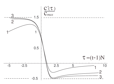
Figure 2:  Derivative of the heat capacity as a function of the (scaled) temperature for different numbers of particles in the system: $N=10^{3}$ (1), $N=10^{6}$ (2), $N\to\infty$ (3).

At arbitrarily low but fixed deviations of the temperature from $T_{\rm BEC}$ ($t=1+\delta t$) the variable $y$ (2.31) has substantially different dependence on $N$ for different signs of the deviation $\delta t$:

$$y=\frac{1}{N}\,\frac{1}{\delta t^{3}}\ll 1,\quad\delta t>0,$$

$$y=-N^{1/3}\delta t\gg 1,\quad\delta t<0.$$

Accordingly, from (2.32) we obtain the following expression for the jump of the derivative of the specific heat $\Delta c^{\prime}=c^{\prime}(1-\delta t)-c^{\prime}(1+\delta t)$ at $N\to\infty$, $\delta t\to 0$:

$$\Delta c^{\prime}=\frac{3}{2}\,c_{max}\,\gamma=\frac{9}{16\pi}\zeta^{2}(3/2),$$

which agrees with the known expression given in [3]. Returning to the ordinary, unnormalized temperature, we can see that the function $c^{\prime}$ for $N\to\infty$ goes over to a $\theta$ function with a “tooth” formed by the minimum on the curve (Fig. 2).

Based on the given calculations, we stress that for BEC as a phase transformation phenomenon it is also necessary to have not too low temperatures at a fixed density of the Bose gas, so as to have a large number of (quasi)particles in the system Therefore, for experimental study of BEC it is preferable to increase the density of excitations at a specified value of $T$, as is done in Ref. [18].

3 Bose condensation in thin films with anisotropic spin-wave spectrum

A study of magnons in ferromagnetic microfilms with dimensions [18]

$$L_{x}\simeq 10\mu m,\quad L_{y}=L_{z}\simeq 1{\text{ }}$$ (3.1)

in a magnetic field directed along the surface of the sample, $\mathbf{H}||z$ , was reported in Ref. 18 (see Fig. 1). The spectrum of long-wavelength spin excitations in real ferromagnets is rather complex. The corresponding dispersion relation $\varepsilon(\mathbf{p})$ differs markedly from (2.5), which describes free massive particles. The additional contributions to $\varepsilon(\mathbf{p})$ are generated by an external magnetic field and the magnetic dipole component of the interaction between spins. In the next Section the influence of these contributions on the BEC process are analyzed in more detail. In the simplest approximation one may keep only the fact that a magnetic-field gap appears in the dispersion relation, so that

$$\varepsilon(\mathbf{p})=\frac{\mathbf{p}^{2}}{2m}+\varepsilon_{\mathbf{H}}\,,$$ (3.2)

where $\varepsilon_{\mathbf{H}}=2\pi\hbar\nu_{\mathbf{H}}$ is the gap energy, its frequency practically coinciding with the ferromagnetic resonance (FMR) frequency. The presence of a gap in the dispersion relation does not affect the thermodynamics of the system, since this is only a shift of the energy (frequency) scale. As is easily seen from the definition (2.9) of $n_{0}$, the substitution $\varepsilon\to\varepsilon+\varepsilon_{\mathbf{H}}$ and $\mu\to\mu+\varepsilon_{\mathbf{H}}$ leaves $n_{0}$, the number of particles on the lowest level, which essentially corresponds to the FMR, practically unchanged. And because it is $n_{0}$, not the chemical potential, that we use as the independent variable, all of the thermodynamic expressions of the previous Section remain in force. The quantity $\varepsilon_{\mathbf{H}}$ is conveniently used as a scale for parameters with dimensions of energy, if only because the diagnostics of the spectral density of of magnons in YIG in [18] was carried out at frequencies $\nu_{\mathbf{H}}\simeq 2\,{\rm GHz}$, in the vicinity of the FMR. Then, e.g., the temperature is given as $T=t/\varepsilon_{\mathbf{H}}$, which implies that, on the scale of quantities corresponding to those typical of [18], a temperature of 1  corresponds to a value $t\simeq 10$. In the dimensionless quantities dispersion relation (3.2) takes the form

$$\varepsilon(\mathbf{p})\equiv\varepsilon_{\mathbf{k}}=\varepsilon_{\mathbf{H}}(1+\omega_{\mathbf{k}})\,,\quad\omega_{\mathbf{k}}=\sum_{j}\omega_{j}k_{j}^{2}\,,$$ (3.3)

where $\omega_{j}=\varepsilon_{j}/\varepsilon_{\mathbf{H}}$, the $\varepsilon_{j}$ being defined in (2.5). In the case of film dimensions (3.1) and magnon masses $m_{m}\simeq 5m_{e}$, corresponding to YIG [10], the numerical values of the parameters $\omega_{j}$ are

$$\omega_{x}\simeq 10^{-4},\quad\omega_{y}=\omega_{z}\simeq 10^{-10}.$$ (3.4)

In the experiments of [18], direct measurements were made of the magnon spectral density

$$n(\omega)=\sum_{\mathbf{k}}n_{\mathbf{k}}\delta(\omega-\omega_{\mathbf{k}})=\frac{g(\omega)}{\mbox{e}^{(\omega-\omega_{0})/t}(1+n_{0}^{-1})-1}\,$$ (3.5)

with high resolution in the long-wavelength part of the spectrum, which is the most important and informative in the context of BEC. The magnon energy was determined from the frequency $\nu=\nu_{\mathbf{H}}(1+\omega)$, and the number of magnons from the intensity of the emission in processes of inelastic Raman scattering of a light wave on the magnon distribution established in the film.

On the right-hand side of (3.5) we have introduced the spectral density of states

$$g(\omega)=\sum_{\mathbf{k}}\delta(\omega-\omega_{\mathbf{k}}).$$ (3.6)

Because of the large difference in the longitudinal and transverse dimensions of the film, the ratio of the corresponding parameters $\omega_{j}$ is also large: $\omega_{x}/\omega_{y}=\omega_{x}/\omega_{z}\sim 10^{6}$. This leads to the circumstance that the spectrum of states is split into layers around the harmonics corresponding to the first component of the quasimomentum. This peculiar structure of the spectrum allows one to decompose $g(\omega)$ and, hence, $n(\omega)$ into three characteristic terms with different singular behavior in the low-frequency (near $\nu_{\mathbf{H}}$) region:

$$g(\omega)=g_{C}(\omega)+g_{1}(\omega)+g_{\infty}(\omega)\,,$$ (3.7)

where

$$g_{C}(\omega)=\delta(\omega-\omega_{0})$$ (3.8)

is the term corresponding to the contribution in (3.6) from the lowest magnon state;

$$g_{1}(\omega)={\sum_{\ \mathbf{k}_{\perp}}}^{\prime}\delta(\omega-\omega_{x}-\omega_{y}\mathbf{k}_{\perp}^{2})\,,\quad\mathbf{k}_{\perp}^{2}=k_{y}^{2}+k_{z}^{2}\,,$$ (3.9)

is the contribution of the first excited layer (the fundamental harmonic of the first component of the quasimomentum) and, finally,

$$g_{\infty}(\omega)=\sum_{k_{x}=2}^{\infty}\sum_{\ \,\mathbf{k}_{\perp}}\delta(\omega-\omega_{x}k_{x}^{2}-\omega_{y}\mathbf{k}_{\perp}^{2})\,$$ (3.10)

is the contribution of all the other states. The prime on the summation sign in (3.9) means that the term with $\mathbf{k}_{\perp}^{2}=2$ is excluded, as it is taken into account explicitly in (3.8). Changing from sums to integrals in (3.9) and (3.10), we obtain

$$g_{1}(\omega) \simeq \frac{\pi}{2}\int\limits_{\sqrt{\varkappa+2}}^{\infty}dk\,k\,\delta(\omega-\omega_{x}-\omega_{y}k^{2})=\frac{\pi}{4\omega_{y}}\theta(\omega-\omega_{x}-\varkappa\omega_{y})\,,$$ (3.11)

$$g_{\infty}(\omega) \simeq \frac{\pi}{2}\sum_{k_{x}=2}^{\infty}\int\limits_{0}^{\infty}dk\,k\,\delta(\omega-\omega_{x}k_{x}^{2}-\omega_{y}k^{2})=\frac{\pi}{4\omega_{y}}\sum_{k_{x}=2}^{\infty}\theta(\omega-\omega_{x}k_{x}^{2})=$$ (3.12)

$$= \frac{\pi}{4\omega_{y}}\biggl{(}\sqrt{\frac{\omega}{\omega_{x}}}-\biggl{\{}\sqrt{\frac{\omega}{\omega_{x}}}\biggr{\}}-1\biggr{)}\theta(\omega-4\omega_{x})\,,$$

where $0<\varkappa<3$, and the curly brackets on the right-hand side of (3.12) denote the fractional part of the quantity enclosed in them (i.e., $\{s\}$ is the fractional part of the real variable $s$). Since $0<\{s\}<1$, one can set the mean value of $\{s\}\simeq 1/2$, which gives for (3.12)

$$g_{\infty}(\omega)=\frac{\pi}{4\omega_{y}\sqrt{\omega_{x}}}\left(\sqrt{\omega}-\frac{3}{2}\sqrt{\omega_{x}}\right)\theta(\omega-4\omega_{x})\,.$$ (3.13)

The partial contribution of $g_{1}(\omega)$ (3.11) is proportional to the surface area of the sample, while in $g_{\infty}(\omega)$ (3.13) the first term is proportional to the volume and the second to the area. Collecting the corresponding terms, we write $g(\omega)$ in the following form:

$$g(\omega)=g_{C}(\omega)+g_{S_{V}}(\omega)+g_{V}(\omega)\,,$$ (3.14)

where

$$g_{C}(\omega) = \delta(\omega-\omega_{0})\,,$$ (3.15)

$$g_{S_{V}}(\omega) = \frac{\pi}{4\omega_{y}}\ [\theta(\omega-\omega_{0}-\varkappa\omega_{y})-\frac{3}{2}\,\theta(\omega-4\omega_{x})]\,,$$ (3.16)

$$g_{V}(\omega) = \frac{\pi\sqrt{\omega}}{4\omega_{y}\sqrt{\omega_{x}}}\ \theta(\omega-4\omega_{x})\,.$$ (3.17)

It is easily checked that for large $\omega$ the phase volume element

$$d\Phi=[g_{V}(\omega)+g_{S_{V}}(\omega)]d\omega$$

agrees with the asymptotic estimate (2.14. However, in the low-energy (threshold ) region of interest to us, the question of the lower limits of integration over the phase volume becomes fundamental, and the answer to this question is contained in expressions (3.15)–(3.17).

In sum, by substituting the formulas obtained for $g(\omega)$ into (3.5), we get

$$n(\omega)=n_{C}(\omega)+n_{S_{V}}(\omega)+n_{V}(\omega)\,,$$ (3.18)

where, in accordance with decomposition (3.14), the functions

$$n_{C}(\omega) = n_{0}\delta(\omega-\omega_{0})\,,$$ (3.19)

$$n_{S_{V}}(\omega) = \frac{\pi}{4\omega_{y}}\ \frac{\theta(\omega-\omega_{0}-\varkappa\omega_{y})-(3/2)\,\theta(\omega-4\omega_{x})}{\bigl{(}1+n_{0}^{-1}\bigr{)}\exp(\frac{\omega-\omega_{0}}{t})-1}\,,$$ (3.20)

$$n_{V}(\omega) = \frac{\pi}{4\omega_{y}\sqrt{\omega_{x}}}\ \frac{\sqrt{\omega}\ \theta(\omega-4\omega_{x})}{\bigl{(}1+n_{0}^{-1}\bigr{)}\exp(\frac{\omega-\omega_{0}}{t})-1}\,,$$ (3.21)

specify the partial frequency distributions corresponding to the condensate, surface, and volume contributions. In a restricted range of frequencies $\omega$ not exceeding a certain value $\omega_{max}$, expressions (3.20) and (3.21) simplify if $n_{0}\gg 1$ and $t\gg\omega_{max}$:

$$n_{S_{V}}(\omega) = \frac{\pi t}{4\omega_{y}}\ \frac{\theta(\omega-\omega_{0}-\varkappa\omega_{y})-(3/2)\,\theta(\omega-4\omega_{x})}{\omega-\omega_{0}+t/n_{0}}\,,$$ (3.22)

$$n_{V}(\omega) = \frac{\pi t}{4\omega_{y}\sqrt{\omega_{x}}}\ \frac{\sqrt{\omega}\ \theta(\omega-4\omega_{x})}{\omega-\omega_{0}+t/n_{0}}\,.$$ (3.23)

It is seen from these expressions that because of the small parameter $\sqrt{\omega_{x}}$ in the denominator of (3.23), the contribution (3.22) from the surface term in the general case is negligible:
$n_{V}(\omega)\gg n_{S_{V}}(\omega)$. But at the thresholds ($\omega=\omega_{0}+\varkappa\omega_{y}$ and $\omega=4\omega_{x}$ for (3.22) and (3.23), respectively) the situation is the opposite: $n_{S_{V}}\gg n_{V}$.

In real experiments the results of measurements depend on the resolving power of the device, and usually one observes not $n(\omega)$ but the spectral density averaged over some frequency interval $\delta\omega\simeq Q^{-1}$:

$$n^{obs}(\omega)=\int\limits_{-\infty}^{\infty}d\omega^{\prime}n(\omega^{\prime})F(\omega-\omega^{\prime})\,,\quad\int\limits_{-\infty}^{\infty}d\omega F(\omega)=1,$$ (3.24)

where $F(\omega)$ is the amplitude frequency characteristic (AFC) of the receiver. Because the value of $n_{C}(\omega)$ in (3.19) is proportional to a $\delta$ function, the observable condensate contribution

$$n^{obs}_{C}(\omega)=n_{0}F(\omega-\omega_{0})$$ (3.25)

actually reproduces the AFC. Expressions (3.24) and (3.25) show that the formation of the resonance peak as the BEC signal involves the participation not of just one state but also of other states whose energies are close to the gap $\varepsilon_{\mathbf{H}}$. Therefore, at some distance from the “condensate” frequency $\omega_{0}$ and not only at the thresholds, the partial contributions $n^{obs}_{S_{V}}(\omega)$ and $n^{obs}_{V}(\omega)$ can have values comparable to $n^{obs}_{C}(\omega)$, despite the quantitative difference in the coefficients in expressions (3.22) and (3.23). Furthermore, owing to the finite width of the AFC the observable magnon spectral density $n^{obs}(\omega)$ is nonzero even in the region below the threshold ($\omega<0$, $\nu<\nu_{\mathbf{H}}$). As the AFC we consider the often-encountered function

$$F(\omega)=\frac{1}{\pi}\,\frac{Q}{1+Q^{2}\omega^{2}}\,.$$ (3.26)

where $Q$ is the quality factor. The integrals (3.24) of the functions (3.22), (3.23), and the Lorentzian (3.26) are taken explicitly. Taking into account the smallness of the parameters $\omega_{x}$, $\omega_{y}$ and $t/n_{0}$ and assuming that $Q\omega_{0}\ll 1$, we arrive at the expressions

$$n^{obs}(\omega) = n^{obs}_{C}(\omega)+n^{obs}_{V}(\omega)+n^{obs}_{S_{V}}(\omega)\,,$$ (3.27)

$$n^{obs}_{C}(\omega) = \frac{n_{0}}{\pi}\,\frac{Q}{1+Q^{2}\omega^{2}}\,,$$ (3.28)

$$n^{obs}_{V}(\omega) = \frac{\pi\,t}{4\sqrt{2}\omega_{y}\sqrt{\omega_{x}}}\biggl{(}\frac{Q^{2}\omega}{1+Q^{2}\omega^{2}}+\frac{Q}{\sqrt{1+Q^{2}\omega^{2}}}\biggr{)}^{1/2}\,,$$ (3.29)

$$n^{obs}_{S_{V}}(\omega) = \frac{t}{8\omega_{y}}\,\frac{Q}{1+Q^{2}\omega^{2}}\biggl{[}A-Q\omega\biggl{(}\frac{\pi}{2}+{\mathrm{arctg\,}}Q\omega\biggr{)}-\frac{1}{2}\ln(1+Q^{2}\omega^{2})\biggr{]}\,,$$ (3.30)

where $A$ denotes the $\omega$-independent quantity (which depends on $T$, $n_{0}$, and the linear dimensions of the system)

$$A=3\ln(t/n_{0}+3\omega_{x})-2\ln(t/n_{0}+\varkappa\omega_{y})+\ln Q\,.$$ (3.31)

It can be seen from expressions (3.28)–(3.31) that the differential components of the spectral density behave differently upon variation of the temperature, film thickness, and the pumping done to produce magnons in sufficient number for BEC in the system. This satisfies the basic prerequisites for reliable separation of the condensate (coherent) component and the surface and volume (incoherent) components of the observed total (and, in essence, unified) spectral curve.

It is extremely significant that in its main details the shape of the spectrum does not depend separately on the temperature and pumping but on their ratio $t/n_{0}$. Expressions (3.28)–(3.31) show that the shape of the $n^{obs}(\omega)$ curve is invariant with respect to simultaneous variation of temperature and the number of particles in the condensate, provided that their ratio $\eta=t/n_{0}$ is constant: at a fixed value of $\eta$ variation of the temperature or magnon pumping affects only a coefficient that is common to all contributions.

The critical magnon density $\mathfrak{n}_{\rm BEC}$ (the derivative of the specific heat as a function of $\mathfrak{n}$) jumps at the transition through $\mathfrak{n}_{\rm BEC}$) has the form

$$\mathfrak{n}_{\rm BEC}=\frac{\zeta(3/2)}{\lambda^{3}_{T}}\,.$$ (3.32)

At room temperature $T=300\,K$ and $m_{m}=5\,m_{e}$ the thermal length (see (2.21) is small: $\lambda_{T}\simeq 1.92\times 10^{-7}$. Therefore the number of particles in the condensate is already quite large: ( $N_{\rm BEC}/V\simeq 6.28\times 10^{14}$, and the parameter $\eta_{\rm BEC}=t/N_{\rm BEC}\simeq 2.9\times 10^{-8}$ is sufficiently small as to ensure the validity of the approximations made in the derivation of (3.28)–(3.31). Despite the large number of particles in the condensate, its contribution to $n^{obs}(\omega)$ is practically unnoticeable (roughly three or four orders of magnitude smaller than the thermal excitations). Nevertheless, please note that the $n^{obs}(\omega)$ curve already shows a completely formed peak as a consequence of the singular (at $\eta\,,\omega\rightarrow 0$) behavior of the surface (3.22) and volume (3.23) contributions to $n^{obs}(\omega)$. For direct observation of $n^{obs}_{C}(\omega)$ in the spectral density it is necessary that $n_{0}\gg N_{\rm BEC}$.

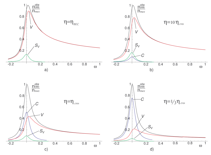
Figure 3:  Spectral density of magnons and its partial contributions at different values of the parameter $\eta$; $n_{max}$ is the normalized coefficient corresponding to the maximum of the total spectral density at the given $\eta$; $L_{x}=10~{}\mu m$, $\eta_{\rm BEC}\simeq 4.8\times 10^{-9}$, $\eta_{cros}\simeq 1.92\times 10^{-12}$; the symbols $C,\,S_{V}$, and $V$ denote the corresponding partial contributions.

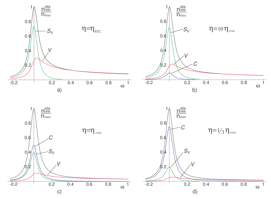
Figure 4:  The same as in Fig. 3, for $L_{x}=1~{}\mu m$; $\eta_{\rm BEC}\simeq 2.22\times 10^{-8}$, $\eta_{cros}\simeq 5.26\times 10^{-12}$.

It can be determined from (3.28)–(3.31) that at such values of the parameter $\eta=\eta_{cros}$ the number of particles in the condensate becomes macroscopic — e.g., equal to the volume contribution of the thermalized excitations. This gives a rough but simple estimate:

$$\eta_{cros}=\frac{4\omega_{y}}{\pi^{2}}\sqrt{2Q\omega_{x}}\,.$$ (3.33)

For a film thickness $L_{x}=10\mu m$ this gives $\eta_{cros}\simeq 2.56\times 10^{-12}$. When the parameter $\eta$ reaches the value $\eta_{cros}$ (with increasing magnon pumping) a kind of crossover occurs, i.e., the peak on the $n^{obs}(\omega)$ curve rises up sharply. A more accurate estimate for $\eta_{cros}$ can be obtained from the quantity $n^{obs}_{C}(0)=n^{obs}_{ex}(\omega_{max})$, where $n^{obs}_{ex}(\omega)=n^{obs}_{V}(\omega)+n^{obs}_{S_{V}}(\omega)$ and $\omega_{max}$ is the frequency at which the function $n^{obs}_{ex}(\omega)$ reaches a maximum. Hence we obtain $\eta_{cros}\simeq 1.92\times 10^{-12}$ for $L_{x}=10\mu m$, and $\eta_{cros}\simeq 5.26\times 10^{-12}$ for $L_{x}=1\mu m$.

¿From these estimates one is convinced that at room temperature, $t=3\cdot 10^{3}$, this crossover occurs at $n_{0}\simeq 1.56\times 10^{15}$ or a density $n_{0}/V\approx 1.56\times 10^{18}\,{cm}^{-3}$, a value which has been attained in YIG films [18].

The above-discussed details of the behavior of the magnon spectral density as a function of $n_{0}$ (which corresponds to the dependence on the pumping level) are illustrated in Figs. 3–5. Figure 3 shows the spectrum corresponding to a microfilm (investigated in [18]) of thickness $\approx 10\mu m$, and Fig. 4 to a film an order of magnitude thinner, $\approx 1\mu m$. It is seen that in the thicker film at all pumping levels the surface contribution is less than the volume contribution, and, essentially, one can speak of only the competition of the condensate and volume contributions. The latter of these, being asymmetric with respect to the maximum and rather strong in the region of the short-wavelength wing of the spectrum, weakens, yielding its place to the condensate contribution that ultimately determines the shape of the band at the highest pumping level (Fig. 3d).

More interesting, perhaps, is the picture of the formation of the spectrum in a very thin film (Fig. 4), when all three contributions are present and competing. Moreover, the surface contribution, as we see, even at relatively weak pumping (Fig. 4a,b) not only remains larger but is essentially dominant, and together with the rising condensate contribution it largely determines the observed shape of the curve. Unlike the case shown in Fig. 3, here the volume contribution, which is also asymmetric, is relatively small (especially at large $n_{0}$), and the condensate contribution mainly “combats” the surface contribution, prevailing only at the highest pumping levels (Fig. 4d). Figures 3 and 4 clearly attest to the possibilities opened up in the study of BEC not only in thin magnetic films but also in other systems of finite size and with a small number of particles.

Finally, Fig. 5 shows the evolution of the total distribution as the temperature is varied, leading, under otherwise equal conditions, to substantial growth of the number of magnons in the condensate with decreasing temperature.

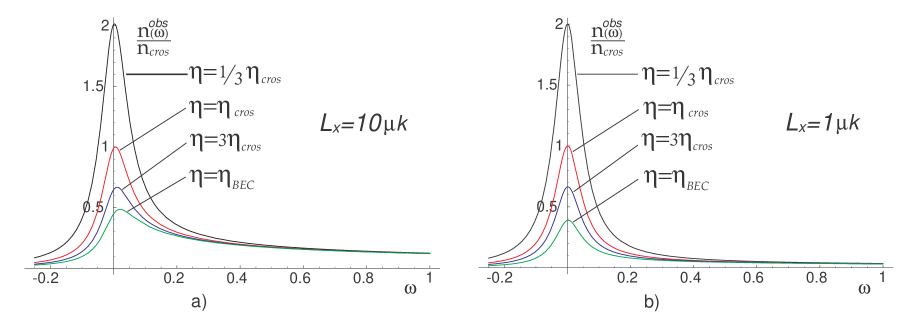
Figure 5:  Total spectral density of magnons at different values of the parameter $\eta$. $n_{cros}$ is the normalized coefficient corresponding to the maximum of the total spectral density at $\eta=\eta_{cros}$.

It should be kept in mind that the crossover point $\eta_{cros}$ here cannot be interpreted as a phase transition signal. In the dimensionless variables used, the temperature of the latter, (1.1), is given by the expression

$$t_{\rm BEC}=\frac{k_{B}T_{\rm BEC}}{\varepsilon_{\mathbf{H}}}=\frac{4}{\pi}(\omega_{x}\omega_{y}\omega_{z})^{1/3}\biggl{[}\frac{N}{\zeta(3/2)}\biggr{]}^{2/3}\,.$$ (3.34)

As was shown above (see Eq. (3.32)), the number of particles of the condensate at the phase transition point is $N_{\rm BEC}\sim N^{2/3}$, and so

$$\eta_{\rm BEC} = \frac{t_{\rm BEC}}{n_{\rm BEC}}=\frac{4}{\pi}\,\frac{(\omega_{x}\omega_{y}\omega_{z})^{1/3}}{\zeta^{2/3}(3/2)}\,,$$

$$\frac{\eta_{cros}}{\eta_{\rm BEC}} = \frac{\zeta^{2/3}(3/2)}{\pi}\sqrt{2Q}(\omega_{x}\omega_{y}\omega_{z})^{1/6}\ll 1.$$ (3.35)

This, in turn, indicates that the appearance of a noticeable peak in the spectral density essentially occurs already in the BEC phase. For the present case of a film with $L_{x}\simeq 10\mu m$, $L_{y}=L_{z}\simeq 1$ cm and for $Q\simeq 20$ the ratio $\eta_{cros}/\eta_{\rm BEC}=N_{\rm BEC}/n_{cros}\simeq 4\cdot 10^{-4}$. In other words, at a fixed temperature a significantly lower density is necessary for a phase transition to the state with the condensate than for observation of the crossover, i.e., the transition to the state with a predominant number of particles in the condensate (see Figs. 3 and 4).

It should be emphasized that the contribution $n^{obs}_{S_{V}}(\omega)$ (3.30) to the spectral density is a mesoscopic or finite-size effect that is isolated in analytical form. One notices that the frequency dependence of this contribution is practically no different from $n^{obs}_{C}(\omega)$. Meanwhile, the physical nature of these contributions is different: $n^{obs}_{C}(\omega)$ is just the contribution of a large number of magnons with identical quantum numbers. This set of quasiparticles is a quantum object consisting of a macroscopic number of particles, or a coherent Bose condensate. On the contrary, $n^{obs}_{S_{V}}(\omega)$ is formed of a set of magnons with different quantum numbers and corresponds to an obviously incoherent state.

It is scarcely possible to distinguish these contributions by the attribute of coherence with the aid of the corresponding interference measurements. Nevertheless, because the contribution $n^{obs}_{S_{V}}(\omega)$ is proportional to the temperature and the surface area of the sample [unlike $n^{obs}_{C}(\omega)$], these components of the spectral density can be distinguished with the aid of a series of measurements at different temperatures on samples of different size and shape.

For a quantitative description of the data it is necessary, among other things, to have information on the effective AFC of the measuring setup. The Lorentzian (3.26) that we used as a model can scarcely correspond to reality. Nevertheless, even in this simple model one sees a substantial dependence of the results of observation on the parameters of the AFC, in the present case—on the quality factor $Q$. Considering the partial contributions as functions of the reduced frequency $Q\,\omega$, it is easy to see that the contribution of the condensate goes as $\sim Q$, while the volume contribution (3.29) goes as $\sim Q^{1/2}$. Therefore, with increasing resolving power the contribution of the condensate becomes more and more noticeable against the background of the volume component. This can be used for identification of the volume component. However, the surface contribution is also practically proportional to the factor, and therefore variation of the $Q$ factor is insufficient for separating it from the condensate component, and special data processing is necessary (such as that mentioned above).

4 Inclusion of anisotropy of the magnon dispersion relation

As we have said, in real ferromagnetic films, because of the contribution of the magnetic dipole interaction, the spectrum of long-wavelength magnons is anisotropic. Here the anisotropy is determined by the external magnetic field, which sets the magnetization direction [10, 18]. Taking that interaction into account leads to a distortion of the isotropic quadratic dispersion relation (3.3) such that its dependence on the third component of the quasimomentum exhibits a characteristic dip (see Fig. 6) at a value $p_{z}=p_{0}\simeq 3\cdot 10^{-4}\,cm^{-1}$ (recall that ${\mathbf{H}}||z$).

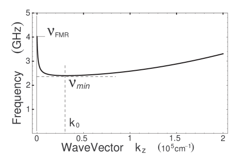
Figure 6:   Form of the dispersion relation of long-wavelength magnons with wave vectors $\mathbf{k}||\mathbf{H}$ in a ferromagnetic microfilm.

The corresponding $\varepsilon({\mathbf{p}})$ dependence is well approximated by the expression

$$\varepsilon(\mathbf{p})=\frac{{\mathbf{p}}^{2}}{2m}+\frac{\varepsilon(0)}{p_{z}/p_{a}+1}\,,$$ (4.1)

which for $p_{a}\rightarrow\infty$ and $\varepsilon(0)\rightarrow\varepsilon_{\mathbf{H}}$ goes over to (3.2). If one knows the energy at zero, $\varepsilon(0)$, and the parameters of the extremum, $p_{0}$ and $\varepsilon_{0}\equiv\varepsilon(p_{0})$, then the momentum $p_{a}$ on the right-hand side of (4.1) can be written in the form

$$\frac{p_{0}}{p_{a}}=\frac{\varepsilon(0)}{\varepsilon_{0}-p_{0}^{2}/2m}-1.$$ (4.2)

In accordance with the phenomenological curve in Fig. 6 we have: $\varepsilon(0)/2\pi\hbar\simeq 4$GHz, $\varepsilon_{0}/2\pi\hbar\simeq 2.3$GHz. However, for the sake of unification in the case considered above we assume that the energy at the minimum, $\varepsilon_{0}$, corresponds to the gap energy $\varepsilon_{\mathbf{H}}$ of the previous Section ($\varepsilon_{0}/2\pi\hbar\simeq 2$GHz). Then Eq. (4.1) is written in dimensionless variables as

$$\varepsilon({\mathbf{p}}) \equiv \varepsilon_{\mathbf{k}}=\varepsilon_{0}(1+\omega_{\mathbf{k}}),\quad\omega_{\mathbf{k}}=\omega_{x}k_{x}^{2}+\omega_{y}k_{y}^{2}+\omega_{z}\,f(k_{z}),$$

$$f(k_{z}) = (k_{z}-k_{0})^{2}\biggl{(}1+\frac{2k_{0}}{k_{z}+k_{a}}\biggr{)}=k_{z}^{2}+\frac{2k_{0}(k_{0}+k_{a})^{2}}{k_{z}+k_{a}}-k_{0}(3k_{0}+2k_{a}),$$ (4.3)

where

$$k_{0}\simeq 10^{4},\quad k_{a}\simeq 270.$$

We note that the minimum of energy in (4.3) corresponds to the state with quantum numbers k$\mathbf{k}=(1,1,k_{0})$.

Calculation of the spectral density of the number of states

$$g(\omega)=\sum_{{\mathbf{k}}}\delta(\omega-\omega_{\mathbf{k}})$$

with the anisotropic dispersion relation (4.3) is complicated considerably in comparison with the simple calculations in Sec. III. Nevertheless, the final expressions are quantitatively very close to those obtained for the isotropic case. Repeating the calculation scheme of the previous Section, we separate out from $g(\omega)$ the lowest state $g_{C}(\omega)$, the contribution of the first ($(k_{x}=1)$) harmonic $g_{1}(\omega)$, and the remaining part $g_{\infty}(\omega)$:

$$g(\omega)=g_{C}(\omega)+g_{1}(\omega)+g_{\infty}(\omega),$$

$$g_{C}(\omega)=\delta(\omega-\omega_{x}-\omega_{y}),$$

$$g_{1}(\omega) = {\sum_{{\mathbf{k}}_{\perp}}}^{\prime}\delta[\omega-\omega_{x}-\omega_{y}k_{y}^{2}-\omega_{z}f(k_{z})]\simeq$$ (4.4)

$$\simeq \frac{J(\omega)}{2\sqrt{\omega_{y}\omega_{z}}}\,\theta(\omega-\omega_{x}-\omega_{y})\,.$$

The notation $J(\omega)$ on the right-hand side of (4.4) stands for the integral (which is evaluated in Appendix B)

$$J(\omega)=\int\limits_{z_{1}}^{z_{2}}\frac{dz}{\sqrt{\omega-\omega_{x}-w(z)}}\,,$$ (4.5)

where $z_{1}$ and $z_{2}$ are roots of the equation $w(z)=\omega-\omega_{x}$:

$$w(z)=\omega_{z}f(z/\sqrt{\omega_{z}})=(z-z_{0})^{2}\biggl{(}1+\frac{2z_{0}}{z+z_{a}}\biggr{)},$$ (4.6)

where $z_{a}=k_{a}\sqrt{\omega_{z}}\simeq 2.7\cdot 10^{-3}$, $z_{0}=k_{0}\sqrt{\omega_{z}}\simeq 10^{-1}$.

In an analogous way, by calculating the contribution $g_{\infty}(\omega)$ to accuracy $O(\sqrt{\omega_{x}})$, we find

$$g_{\infty}(\omega) = \sum_{k_{x}=2}^{\infty}\sum_{\ \ {\mathbf{k}}_{\perp}}\delta[\omega-\omega_{x}k_{x}^{2}-\omega_{y}k_{y}^{2}-\omega_{z}f(k_{z})]\simeq$$ (4.7)

$$\simeq \frac{\theta(\omega-4\omega_{x}-\omega_{y})}{2\sqrt{\omega_{x}\omega_{y}\omega_{z}}}\,\biggl{[}\frac{\pi}{2}(z_{2}-z_{1})-\frac{3}{2}\sqrt{\omega_{x}}J(\omega)\biggr{]}\,.$$

Collecting terms proportional to the surface and volume in (4.4) and (4.4), we obtain (cf. (3.16) and (3.17)):

$$g_{S_{V}}(\omega) = \frac{J(\omega)}{2\sqrt{\omega_{y}\omega_{z}}}\ [\theta(\omega-\omega_{x}-\omega_{y})-\frac{3}{2}\,\theta(\omega-4\omega_{x}-\omega_{y})]\,,$$ (4.8)

$$g_{V}(\omega) = \frac{\pi~{}(z_{2}-z_{1})}{4\sqrt{\omega_{x}\omega_{y}\omega_{z}}}\ \theta(\omega-4\omega_{x}-\omega_{y})\,.$$ (4.9)

It is easily checked that the integral $J(\omega)$, generally speaking, depends weakly on $\omega$; for example, for $\omega\gg\omega_{x}$ the function $J(\omega)\simeq\pi/2$, which coincides with our previous investigation of the isotropic case. A quantitative difference, though slight, appears only in the region of very low frequencies (near the threshold), as is illustrated in Fig. 7.

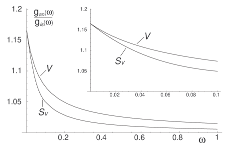
Figure 7:  Ratio of spectral densities of states: $g_{an}(\omega)$ corresponds to the anisotropic dispersion relation (4.1), and $g_{is}(\omega)$ to the isotropic one (3.2); as above, the symbol $V$ denotes the volume contributions, $S_{V}$ the surface contributions.

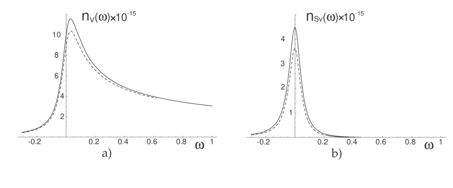
Figure 8:  The volume (a) and surface (b) contributions to the spectral density of magnons for a film 10 $\mu m$ thick; the solid curve corresponds to the anisotropic dispersion relation (4.1), and the dashed curve to the isotropic one (3.2).

Therefore, both the surface and volume contributions to the spectral density of thermal spin excitations (4.7) are quantitatively similar from the case of an isotropic dispersion relation (3.2). On the whole, the observed spectral distribution in this case is qualitatively the same as the curves shown in Figs. 3 and 4.

The calculations done lead to a completely optimistic conclusion for experiment: it would seem that the rather substantial difference in the dispersion relations (3.2) and (4.1) has almost no effect on the results of measurement of the spectral density of magnons, as is illustrated in Fig. 8. Thus the model of an ideal degenerate Bose gas with isotropic quadratic spectrum is completely adequate for interpretation of experiments on the BEC of magnons in real ferromagnetic systems.

5 Conclusion

The calculations done here convincingly demonstrate that in a thin ferromagnetic film with dimensions of $1\,cm\times 1\,cm\times 10\,\mu m$ the BEC of spin excitations can be achieved already at a level of pumping that ensures the appearance and existence of $\sim 10^{15}$ magnons in the film. The fundamental thing is that there are practically no restrictions on temperature, and all the signs of BEC appear at rather high temperatures, including room temperature. Of course, lowering the temperature to the liquid hydrogen or helium region should lower the level of the “critical” pumping in view of the fact that, as we have shown, there is scaling or, in other words, the magnon spectral density depends not on the total number of particles and temperature but only on their ratio $N/T$. The shape of the observable spectrum of long-wavelength magnons remains unchanged when this ratio is held constant. We recall that the number of these quasiparticles is completely specified by the external pumping.

On the other hand, the shape of the measured spectrum is largely connected to the AFC of the filter and can also be varied by improving its $Q$. Its increase (or the segregation of a narrower frequency region around the lowest condensed magnon states) also leads to narrowing of the bandwidth, and consequently, to a more definite investigation specifically of the Bose condensate on whose consituent quasiparticles the Brillouin scattering of the light wave occurs.

In interpreting the experimental data it should be recalled that one cannot claim direct observation of the condensate solely on the basis that a peak appears in the spectral density. All of the contributions have a similar structure, and it is necessary to separate each of them reliably from the experimental data. It follows from the theory that the main distinguishing features of the condensate contribution is its independence of temperature and the size of the sample. Therefore a precise and convincing separation of $n^{obs}_{C}(\omega)$ requires additional measurements at different temperatures.

In studying the BEC phenomenon in magnetic films, we have treated them as systems of finite size. In such systems, as we have said, it is known that BEC occurs not as a phase transition but as crossover. However, the condensation, which occurs near a certain temperature $T_{cros}$, occurs so rapidly that that temperature, though not a critical temperature, can be treated as such. Apparently, the transition could be made more smooth (or smeared in temperature) if an even thinner film were used while the rather high measurement temperature was maintained. Here the absence of a phase transition point in no way precludes the phenomenon of BEC, or the macroscopic accumulation of magnons in their lowest energy state. Moreover, thin films are interesting in still another respect: in them one could trace the role and contribution of the correction terms (see Eq. (2.14)) arising when one goes from summation to integration over phase volume elements, something that, as far as we know, has hitherto escaped attention.

The above calculations of the spectral density of magnons in a ferromagnetic film presuppose the presence of an equilibrium magnon gas, which, strictly speaking, does not correspond to reality. Intense electromagnetic pumping creates relatively short-lived spin excitations, as a result of four-magnon interaction, which, as was shown in [23], rapidly relax to a quasiequilibrium distribution with a temperature equal or nearly equal to the temperature of the crystal (owing to the spin lattice coupling). Consideration of magnon magnon and magnon phonon relaxation processes simultaneously with the process of magnon Bose condensation undoubtedly requires a special analysis and will be done separately.

Finally, we note that it has been proposed in an experimental paper [18] that the accumulation of magnons at two (symmetric) points of the spin-wave spectrum fulfills the prerequisites for a nonuniform Bose condensate. However, from the standpoint of the thermodynamics of the process, no finite number of degenerate points of $\mathbf{k}$ space will affect the observed scattering pattern and the spectral density corresponding to it, which will be completely described in the framework of the approach stated above. This conclusion remains in force, despite the fact that the condensate that arises in such a case can be defined as incoherent. A distinction would arise only in the case when the lowest state of the magnon spectrum for some reason was infinitely degenerate (e.g., this could correspond to a model spectrum in the form of a trough). The condensate corresponding to that case is also incoherent, and the transition to it would have some distinctions. However, the study of the features of such a model is beyond the scope of this paper.

We are sincerely grateful to G.A. Melkov for acquainting us with the results of the experimental study by him and his coauthors, which stimulated our study, and for numerous discussions and constructive criticism.

This study was supported in part by the grant SCOPES N IB7320-110840 SMSF, grant 02.07/00152 of the DFFD of Ukraine, and by the target program of the Department of Physics and Astronomy of the National Academy of Sciences of Ukraine.

APPENDIX A

To demonstrate the problem with not separating the singular term, we consider a series whose sum is expressed in terms of elementary functions:

$$S=\sum_{l=0}^{\infty}\frac{1}{l^{2}+x}=\frac{1}{2x}+\frac{\pi}{2}\,\frac{\coth(\pi\sqrt{x})}{\sqrt{x}}\,.$$

A “naive” transition from the sum to an integral in Eq. (A.1) gives the following approximation for $S$:

$$S\approx S_{0}=\int\limits_{0}^{\infty}\frac{dl}{l^{2}+x}=\frac{\pi}{2\sqrt{x}}\,.$$

If the first term in Eq. (A.1), corresponding to $l=0$, is separated off, and the remaining sum is approximated by an integral, we then get

$$S\approx S_{1}=\frac{1}{x}+\int\limits_{1/2}^{\infty}\frac{dl}{l^{2}+x}=\frac{1}{x}+\frac{\arctan(2\sqrt{x})}{\sqrt{x}}\,,$$

It is easy to check that approximation (A.3) is practically no different from the exact expression (A.1) in the whole range of variation of the parameter $x>0$. Approximation (A.2), on the contrary, is a very crude approximation compared to (A.3), especially at $x\to 0$. For example, one can compare their asymptotic behavior at large and small $x$:

$$x\to 0:\quad S = \frac{1}{x}+\frac{\pi^{2}}{6}-\frac{\pi^{4}x}{90}+O(x^{2})\,,$$

$$S_{1} = \frac{1}{x}+2-\frac{8x}{3}+O(x^{2})\,,$$

$$x\to\infty:\quad S = \frac{\pi}{2\sqrt{x}}+\frac{1}{2x}+O(\mbox{e}^{-2x})\,,$$

$$S_{1} = \frac{\pi}{2\sqrt{x}}+\frac{1}{2x}+\frac{1}{24x^{2}}+O(x^{3})\,.$$

Figure 9 shows graphs of $S$ as a function of the parameter $x$ for the exact and approximate expressions.

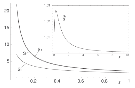
Figure 9:  Behavior of the series $S$ and its approximations $S_{0}$ and $S_{1}$ as functions of the parameter $x$; the inset shows a plot of the ratio $S/S_{1}$.

APPENDIX B

Consider the integral (see (4.5))

$$J(\omega)=\int\limits_{z_{1}}^{z_{2}}\frac{dz}{\sqrt{\omega-w(z)}}\,,$$

where

$$w(z)=(z-z_{0})^{2}\left(1+\frac{2z_{0}}{z+z_{a}}\right)\,.$$

The limits of integration in (B.1) are the positive roots (see Fig. 10) of the equation $w(z_{1,2})=\omega$.

Figure 10:  Graphical solution of the equation $w(z_{1,2})=\omega$.

For calculating the integral, the expression under the square root in (B.1) is conveniently written in the form

$$\omega-w(z)=\frac{(z_{2}-z)(z-z_{1})(z+z_{a}+z_{1}+z_{2})}{z+z_{a}}\,.$$

Then with the standard change of the integration variable

$$z=\frac{z_{1}(z_{2}+z_{a})+z_{a}(z_{2}-z_{1})\sin^{2}\varphi}{(z_{2}+z_{a})-(z_{2}-z_{1})\sin^{2}\varphi}$$

integral (B.1) is transformed to

$$J(\omega)=\frac{2(z_{a}+z_{1})}{\sqrt{(z_{a}+z_{2})(z_{a}+2z_{1}+z_{2})}}\int\limits_{0}^{\pi/2}\frac{d\varphi}{(1-a\sin^{2}\varphi)\sqrt{1-ab\sin^{2}\varphi}}\,,$$

where

$$a=\frac{z_{2}-z_{1}}{z_{a}+z_{2}}\,,\quad b=\frac{z_{2}+z_{1}}{z_{a}+2z_{1}+z_{2}}\,.$$

The integral on the right-hand side of (B.2) is the Legendre complete elliptic integral of the third kind, $\Pi(a,ab)$.

NOTE ADDED IN PROOF

After this article was submitted to Low Temperature Physics, an experimental paper appeared [J. Kasprzak, M. Richard, S. Kundermann, A. Baas, J. M. J. Keeling, F. M. Marchetti, M. H. Szymanska, R. Andre, J. L. Staehli, V. Savona, P. B. Littlewood, B. Deveaud, and Le Si Dang, Nature 443, 409 (2006)] in which the Bose Einstein condensation of quasiparticles was also reported. In that paper a different type of relatively light quasiparticles of the Bose type was considered, specifically, exciton polaritons, a high density of which can be produced by laser pumping in optical microcavities in a CdTe crystal. In it, as in YIG, thermalization of the pumped quasiparticles occurs, and above a certain quasiparticle density there is macroscopic occupation of the quasiparticle (in this case, polariton) ground state, at a rather high critical temperature $T_{\rm BEC}\approx 19$ K. Evidence of Bose condensation is provided by weak coherent correlation effects observed in the radiation emitted from the crystal. There, however, it is not ruled out that additional information about the formation of a Bose condensate specifically could be obtained if the volume and surface contributions to the observed intensity and line shape could be separated (on the basis of their temperature or concentration behavior). Although in our paper these contributions are calculated for magnons, they should undoubtedly also be present for polaritons in the small volumes of the optical microcavities.

References

- [1] S.N. Bose. Z. Phys. 26, 171 (1924).
- [2] A. Einstein. Preuss. Akad. Wiss. Math. Kl. Bericht. 1, 2 (1925).
- [3] L.D. Landau and E.M. Lifshitz. Statistical Physics, Part 1, 3rd ed., Pergamon Press, Oxford (1980), Nauka, Moscow (1976).
- [4] M.H. Anderson, J.R. Ensher, M.R. Matthews, C.E. Wieman, and E.A. Cornell. Science 269, 198 (1995).
- [5] K.B. Davis, M.-O. Mewes, M.R. Andrews, N.J. van Druten, D.S. Durfee, D.M. Kurn, and W. KeHerle. Phys. Rev. Lett. 75, 3969 (1995).
- [6] S.A. Moskalenko, and D.W. Snoke. Bose-Einstein Condensation Excitons and Biexcitons. Cambridge Univ. Press, Cambridge (2000).
- [7] C.D. Jefferies, and L.V. Keldysh. Electron-Hole Droplets in Semi-conductors. Elsevier Sci. Ltd. (1983); L.V. Keldysh. Contem. Phys. 27, 395 (1986).
- [8] J.P. Einstein, and A.H. McDonald. Nature 432, 691 (2004).
- [9] M.I. Kaganov, N.B. Pustyl nik, and T.I. Shalaeva, Usp. Fiz. Nauk 167, 197 (1997).
- [10] A.G. Gurevich, Magnetic Resonance in Ferrites and Antiferromagnets [in Russian], Nauka, Moscow (1973); A.G. Gurevich and G.A. Melkov, Magnitic Oscillations and Waves, CRC Press, Boca Raton, Florida (1996), Nauka, Moscow (1994).
- [11] T. Nikuni, M. Oshikawa, A. Oosawa, and H. Tanaka. Phys. Rev. Lett. 84, 5868 (2000).
- [12] M. Matsumoto, B. Normand, T.M. Rice, and M. Sigrist. Phys. Rev. Lett. 89, 077203 (2003).
- [13] E.Ya. Sherman, P. Lemmens, B. Busse, A. Oosawa, and H. Tanaka. Phys. Rev. Lett. 91, 057201 (2003).
- [14] C. Rüegg, N. Cavadini, A. Furer, H.-U. Güdel, K. Krämer, H. Mutka, A. Wildes, K. Habicht, and P. Vorderwisch. Nature 423, 62 (2003).
- [15] T. Radu, H. Wilhelm, V. Yushanhai, D. Kovrizhin, R. Coldea, Z. Tylczynski, T. Luhmann, and F. Steglich. Phys. Rev. Lett. 95, 1272002 (2005).
- [16] M. Crisan, D. Bodea, I. Tifrea and I. Grosu. Rom. J. Phys. 50, 427 (2005).
- [17] V.M. Kalita and V.M. Loktev, Zh. Eksp. Teor. Fiz. 125, 1149 (2004) [JETP 98, 1006 (2004)].
- [18] S. Demokritov, V. Demidov, O. Dzyapko, G.A. Melkov, A.A. Serga, B. Hillebrands, and A.N. Slavin. Nature 443, 430, (2006).
- [19] A.S. Davydov. Theory of the Solid State [in Russian], Nauka, Moscow (1973).
- [20] A.I. Akhiezer, V.G. Bar yakhtar, and S.V. Peletminskii. Spin Waves, North-Holland, Amsterdam (1968), Nauka, Moscow (1967).
- [21] R.P. Feynman. Statistical Mechanics: a Set of Lectures, Benjamin, Reading, Mass. (1972), Mir, Moscow (1978).
- [22] H. Weyl, Ramifications old and new, of the eigenvalue problem, Bull. Amer. Math. Soc., 56, 115 (1950) [Russ. transl. in Herman Weyl, Selected Works, V.I. Arnol d (ed.), Nauka, Moscow (1984), p. 361].
- [23] Yu.D. Kalafati and V.L. Safonov. JETP Lett. 50, 149 (1989).