A numerical method to solve the Boltzmann equation for a spin valve

Abstract

We present a numerical algorithm to solve the Boltzmann equation for the electron distribution function in magnetic multilayer heterostructures with non-collinear magnetizations. The solution is based on a scattering matrix formalism for layers that are translationally invariant in plane so that properties only vary perpendicular to the planes. Physical quantities like spin density, spin current, and spin-transfer torque are calculated directly from the distribution function. We illustrate our solution method with a systematic study of the spin-transfer torque in a spin valve as a function of its geometry. The results agree with a hybrid circuit theory developed by Slonczewski for geometries typical of those measured experimentally.

1 Introduction

Magnetic multilayer structures have attracted a great deal of experimental and theoretical attention. One motivation for these studies is the potential application of such structures for data storage and spin dependent transistors. One special effect in a magnetic multilayer that can induce magnetic reversal or magnetic dynamics is called spin-transfer. In the ten years since its theoretical prediction, Slonczewski:1996 ; Berger:1996 spin-transfer has been studied extensively both experimentally Katine:2000b ; Urazhdin:2003a ; Kiselev:2003 ; Rippard:2004a ; Fert:2004 and theoretically. Sun:2000 ; Hernando:2000 ; Waintal:2000 ; Stiles:2002b ; Li:2003 ; Bazaliy:2004 One fundamental issue is how to reliably calculate the spin-transfer torque in spin valve systems. To solve this problem, different approaches have been developed, including the Boltzmann equation Stiles:2002a ; Xiao:2004 , microscopic quantum mechanics Edwards:2005 , drift-diffusion theory Berger:1998 ; Grollier:2003 ; Fert:2004 ; Stiles:2004 ; Barnas:2005 , and circuit theory Brataas:2000 ; Brataas:2001 .

Each approach has its own advantages and disadvantages. Simple theories, for example circuit theory or the drift-diffusion approach, treat the transport in terms of densities and current densities and do not track individual electrons. Such methods have the advantage that they can give analytic results in some limits and the disadvantage that they leave out some essential physics. One of the major approximations of these theories is that they ignore the differences between electrons propagating in different directions. Fully quantum mechanical calculations track all of the electrons and all of the coherent scattering processes like coherent multiple scattering between layers. However, such calculations are quite time consuming and the coherent multiple scattering between layers that is included in such an approach does not seem to play a role in experimental results.

The semiclassical Boltzmann equation is a useful compromise between these extremes. In such an approach, the scattering is treated semiclassically. For transport in collinear magnetic systems, it has been used in two ways. Superlattices that have mean free paths longer than layer thicknesses can be treated as artificial bulk materials Zahn:1995 ; Zahn:2005 . This approach retains the coherent multiple scattering between the interfaces. The other approach is to solve the Boltzmann equation within layers and join the solutions through boundary conditions at the interface. Here, we describe a generalization of the latter approach to treat non-collinear magnetizations. In this approach, the Boltzmann equation tracks individual electrons through the distribution function, but ignores the coherent multiple scattering. It is easier to treat defect scattering in such an approach than it is in a fully coherent calculation. The advantage of the Boltzmann calculation is that it is simply computable and includes the essential physics. One disadvantage is that it cannot give analytical results. The neglect of coherent multiple scattering between interfaces is both an advantage and a disadvantage. The greater simplicity that results in the calculation is an advantage for the metallic devices that have been measured to date because the coherent scattering does not appear to play a role. However, this neglect would be a disadvantage in devices in which such effects were important.

Slonczewski has developed a hybrid approach combining aspects of circuit theory with a simplified Boltzmann equation to give an analytic expression for the spin-transfer torque Slonczewski:2002 . This approach gives much more accurate results than the drift-diffusion method for typical device geometries. However, it breaks down when layer thicknesses become longer than are typical.

In this paper, we describe a numerical algorithm that solves the Boltzmann equation for the electron distribution function in a magnetic multilayer system using a scattering matrix formalism. The spin-transfer properties are calculated from the resulting distribution function. We compare our Boltzmann results to the results from more approximate methods. These comparisons show Slonczewski’s hybrid theory is highly accurate for typical experimental structures, but drift-diffusion shows systematic deviations. We have reported results of calculations using the methods described in the present paper in earlier papers Stiles:2002a ; Xiao:2004 .

The paper is organized as follows: Section 2 gives a generalized spin-dependent Boltzmann equation appropriate for ferromagnetic systems; Section 3 describes in detail the algorithm that solves the Boltzmann equation in a spin valve magnetic multilayer system; Section 4 shows the results of the Boltzmann method developed in Section 3 applied to a spin valve. Section 5 gives a summary. Readers who are not interested in the formalism can skip directly to Section 4.

2 Generalized matrix Boltzmann equation

In non-magnetic materials, the spin independent Boltzmann equation is

$${\bf v_{k}}\cdot\frac{\partial g({\bf r,k})}{\partial{\bf r}}-e{\bf E}\cdot{\bf v_{k}}{\partial g({\bf r,k})\over\partial\epsilon_{\bf k}}=\int d{\bf k^{\prime}}P_{\bf k,k^{\prime}}[g({\bf r,k^{\prime}})-g({\bf r,k})],$$ (1)

where $g({\bf r,k})$ is an electron distribution function that depends on the spatial coordinate $\bf r$ and electron wave-vector $\bf k$. ${\bf v_{k}}$ is the electron velocity, $\epsilon_{\bf k}$ its energy, ${\bf E}$ is the electric field, and we have ignored the magnetic field. $P_{\bf k,k^{\prime}}$ is the probability of electron scattering from state ${\bf k^{\prime}}$ to state ${\bf k}$. The Boltzmann equation is valid only when the bulk properties vary slowly. It cannot be used for abrupt interfaces or boundaries; later we describe how to use boundary conditions to relate solutions of the Boltzmann equation in different regions across the interfaces.

Transport in metals is dominated by the electrons near the Fermi energy. The occupancy of states far from the Fermi energy does not change and those states do not contribute to the transport. This suggests the use of the linearized Boltzmann equation in which the distribution function is assumed to have the form

$${g}({\bf r,k})=f_{0}({\bf k})+{f}({\bf r,k})\delta(E_{\rm F}-\epsilon_{\bf k}),$$ (2)

where $f_{0}$ is the equilibrium distribution function. The delta function restricts the wave vector to the Fermi surface, $|{\bf k}|=k_{\rm F}$ for free electrons. With this approximation for the distribution function, the Boltzmann equation becomes

$${\bf v_{k}}\cdot\frac{\partial f({\bf r,k})}{\partial{\bf r}}-e{\bf E}\cdot{\bf v_{k}}=\int_{\rm FS}d{\bf k^{\prime}}P_{\bf k,k^{\prime}}[f({\bf r,k^{\prime}})-f({\bf r,k})],$$ (3)

where the integration over ${\bf k^{\prime}}$ is now a two-dimensional integral restricted to the Fermi surface. The scattering rate $P_{\bf k,k^{\prime}}$ has been rescaled. A delta function has been factored out of each term. In the second term on the left hand side, this delta function comes from $\partial f_{0}/\partial\epsilon$.

For spin dependent magnetic materials, one needs a spin dependent distribution function as well as a spin dependent Boltzmann equation. When there is a natural quantization axis, i.e., all electron spins are either parallel ($\sigma=\uparrow$) or anti-parallel ($\sigma=\downarrow$) to the axis, an electron distribution function is separated into the distribution functions for spin-up and spin-down electrons: $f^{\uparrow}({\bf r,k})$ and $f^{\downarrow}({\bf r,k})$

$${\bf v_{k}}^{\sigma}\cdot{\partial f^{\sigma}({\bf k})\over\partial{\bf r}}-e{\bf E}\cdot{\bf v_{k}}^{\sigma} = \int_{\rm FS}d{\bf k^{\prime}}P_{\bf k,k^{\prime}}^{\sigma}[f^{\sigma}({\bf k^{\prime}})-f^{\sigma}({\bf k})]$$

$$+\int_{\rm FS}d{\bf k^{\prime}}P_{\bf k,k^{\prime}}^{\rm sf}[f^{\sigma^{\prime}}({\bf k^{\prime}})-f^{\sigma}({\bf k})],$$

The $\bf r$ dependence of the distribution function has been suppressed, and $\sigma=\uparrow$, $\downarrow$ and $\sigma\neq\sigma^{\prime}$. Compared with Eq. (3), Eq. (LABEL:eqn:Boltzmann-flip) has an additional spin flip scattering term on the right hand side because the distribution function in Eq. (3) includes both spin types, while the one in Eq. (LABEL:eqn:Boltzmann-flip) is for only one spin type. Similar to the definition of $P_{\bf k,k^{\prime}}$ in Eq. (3), $P_{\bf k,k^{\prime}}^{\sigma}$ and $P_{\bf k,k^{\prime}}^{\rm sf}$ are the probabilities of electron scattering from state ${\bf k^{\prime}}$ to state ${\bf k}$ without and with spin flip. We assume that $P_{\bf k,k^{\prime}}^{\rm sf}$ is the same for spin flip in both directions, up to down or down to up.

In a non-magnet, there is no natural quantization axis, so it is convenient to use the axis of neighboring ferromagnetic layers if the magnetizations of those layers are collinear. In this case, the scattering $P_{\bf k,k^{\prime}}$ is spin-independent, so the substitutions $f^{0}={1\over 2}(f^{\uparrow}+f^{\downarrow})$ and $f^{z}={1\over 2}(f^{\uparrow}-f^{\downarrow})$ give the pair of equations

$${\bf v_{k}}\cdot{\partial f^{0}({\bf k})\over\partial{\bf r}} -e{\bf E}\cdot{\bf v_{k}}= \int_{\rm FS}d{\bf k^{\prime}}P_{\bf k,k^{\prime}}[f^{0}({\bf k^{\prime}})-f^{0}({\bf k})]$$

$$+\int_{\rm FS}d{\bf k^{\prime}}P_{\bf k,k^{\prime}}^{\rm sf}[f^{0}({\bf k^{\prime}})-f^{0}({\bf k})],$$

$${\bf v_{k}}\cdot{\partial f^{z}({\bf k})\over\partial{\bf r}} \hskip 43.36243pt= \int_{\rm FS}d{\bf k^{\prime}}P_{\bf k,k^{\prime}}[f^{z}({\bf k^{\prime}})-f^{z}({\bf k})]$$

$$-\int_{\rm FS}d{\bf k^{\prime}}P_{\bf k,k^{\prime}}^{\rm sf}[f^{z}({\bf k^{\prime}})+f^{z}({\bf k})],$$

In the first equation, spin flip scattering acts as another form of non-flip scattering as far as the number accumulation is concerned. In the second equation, the electric field plays no role because it does not couple to the spin accumulation. In the systems of interest here, the magnetizations are not collinear, so the spin axis in the distribution function can vary with both ${\bf r}$ and ${\bf k}$. However, the generalization is straightforward. The second equation in Eq. (LABEL:eqn:Boltzmann-nmflip) is replicated for each of the other directions in spin space, with $z\rightarrow x,\ y$. The generalization can be derived from a matrix form of the Boltzmann equation in terms of the matrix distribution function

$$\hat{f}({\bf r,k}) = f^{0}\sigma_{0}+f^{x}\sigma_{x}+f^{y}\sigma_{y}+f^{z}\sigma_{z}.$$ (8)

$$= \hat{U}({\bf r,k})\left[\begin{array}[c]{cc}f^{\uparrow}({\bf r,k})&0\\ 0&f^{\downarrow}({\bf r,k})\end{array}\right]\hat{U}^{\dagger}({\bf r,k})$$

where $\sigma_{x},\sigma_{y}$ and $\sigma_{z}$ are Pauli spin matrices, $\sigma_{0}$ is a $2\times 2$ identity matrix, and $\hat{U}$ is a unitary rotation matrix. The rotation matrix allows spin direction to point in an arbitrary direction over the Fermi surface and as a function of position.

In strong ferromagnets, the rotation matrix in Eq. (8) is independent of the position on the Fermi surface or ${\bf k}$ as in Eq. (LABEL:eqn:Boltzmann-flip). This constraint is a consequence of the large difference in the Fermi surfaces for majority and minority electrons in strong ferromagnets. The constraint arises because any transverse spin accumulation in the electrons near the Fermi surface rapidly dissipates. The transverse spins precess in the large exchange field and do so at different rates because of the complicated Fermi surfaces. The precessing transverse components rapidly dephase with respect to each other, leaving no net transverse moment.

3 Formal technique

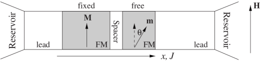
Figure 1: Schematic view of a perpendicular spin valve structure.

Figure 1 shows a schematic picture of a spin valve — a magnetic multilayer structure where a thin-film non-magnet (spacer) is sandwiched between two thin-film ferromagnet (FM) layers. The latter connect to reservoirs with non-magnetic leads. The main purpose of this paper is to solve the Boltzmann equation numerically for the distribution function in such a spin valve structure. In reality, the cross sectional dimensions of these structures are much larger than typical layer thicknesses so that the transport in the interior of the sample is more important than that near the edges. The reservoirs have much larger cross sectional areas and hence smaller resistances than the active structures so that the transport is largely perpendicular to the layers. This combination of features suggests a simple model in which the layers are treated as translationally invariant in plane so that properties only vary perpendicular to the planes. Electrons move in all three directions, but the net current and all variation is in the $x$-direction, i.e. $\hat{f}({\bf r,k})=\hat{f}(x,{\bf k})$.

The calculation proceeds in eight steps: (3.1) discretize the spin dependent Boltzmann equation using a numerical mesh of the Fermi surface; (3.2) solve the discretized Boltzmann equation for the eigensolutions in the non-magnetic and ferromagnetic bulk; (3.3) use the eigensolutions to construct the layer scattering matrix for each bulk layer in the spin valve; (3.4) construct the interface scattering matrix for each interface in the spin valve; (3.5) connect the bulk and interface scattering matrices into a single system-wide scattering matrix; (3.6) determine the boundary conditions and apply them to the system-wide scattering matrix to calculate the distribution function expansion coefficients; (3.7) calculate the distribution function values within the spin valve; and (3.8) calculate the spin density (spin accumulation), spin current, and spin-transfer torque using the distribution function.

3.1 Discretization of the Boltzmann equation

To discretize the Boltzmann equation, we need a numerical mesh for the electron wave-vector $\bf k$ that can accurately and simultaneously describe all Fermi surfaces for both spin types and for all layers. A simple method for choosing a mesh is as follows. Choose a uniform mesh in the direction parallel to the interfaces (perpendicular to $x$): ${\bf k}_{\parallel}^{j}$. For each material, there could be several points on the Fermi surface that have the same ${\bf k}_{\parallel}^{j}$. We label their longitudinal wave-vectors $k_{x}^{n}$. A complete mesh for the Fermi surface is ${\bf k}_{i}=(k_{x}^{n},{\bf k}_{\parallel}^{j})$. The mesh weights are determined by the area on each Fermi surface associated with $k_{x}^{n}$. This mesh may converge slowly, so it may be necessary to refine the ${\bf k}_{\parallel}^{j}$ mesh to include a higher density of points. Let us assume one such mesh has sampling points $\left\{{\bf k}_{i}\right\}_{1}^{N}$ with weighting factor $\left\{w_{i}\right\}_{1}^{N}$. Using this mesh, the integration for any continuous function $h({\bf k})$ on the Fermi surface can be discretized as:

$$\int_{\rm FS}h({\bf k})d{\bf k}=\sum_{i=1}^{N}w_{i}h({\bf k}_{i}).$$ (9)

We discretize the integrations in Eq. (LABEL:eqn:Boltzmann-flip) using this mesh. Assuming the system is one dimensional in $x$ direction, we have a discretized form of the Boltzmann equation:

$${\partial f_{i}^{\sigma}\over\partial x}-eE_{x}=\sum_{j,\sigma^{\prime}}[\hat{V}^{-1}\hat{B}]_{ij}^{\sigma\sigma^{\prime}}f_{j}^{\sigma^{\prime}},$$ (10)

where the subscript $i$ and $j$ mean that $\bf k$ is evaluated at ${\bf k}_{i}$ or ${\bf k}_{j}$, for instance $f_{i}^{\sigma}=f^{\sigma}({\bf k}_{i})$. The velocity matrix $\hat{V}$ and the scattering matrix $\hat{B}$ are $2N\times 2N$ matrices ($N$ from ${\bf k}_{i}$ index, $2$ from spin index) with matrix elements

$$V_{ij}^{\sigma\sigma^{\prime}} = v_{i}^{\sigma x}\delta_{ij}^{\sigma\sigma^{\prime}},$$ (11)

$$B_{ij}^{\sigma\sigma^{\prime}} = w_{j}P_{ij}^{\sigma}\delta_{\sigma\sigma^{\prime}}-{\delta_{ij}^{\sigma\sigma^{\prime}}\over\tau_{i}^{\sigma}}+w_{j}P_{ij}^{\rm sf}(1-\delta_{\sigma\sigma^{\prime}})-{\delta_{ij}^{\sigma\sigma^{\prime}}\over\tau_{i}^{\rm sf}},$$

where $\delta_{ij}^{\sigma\sigma^{\prime}}=\delta_{ij}\delta_{\sigma\sigma^{\prime}}$, $1/\tau_{i}^{\sigma}=\sum_{j}w_{j}P_{ij}^{\sigma}$, is the spin-dependent non-spin-flip scattering rate, and $1/\tau_{i}^{\rm sf}=\sum_{j}w_{j}P_{ij}^{\rm sf}$ is the spin flip scattering rate. See Eq. (LABEL:eqn:Boltzmann-flip). The matrix $\hat{B}$ is singular because $\sum_{j,\sigma^{\prime}}B_{ij}^{\sigma\sigma^{\prime}}=0$.

3.2 Solution of the Boltzmann equation in the bulk

In this section, we briefly summarize the results of Ref. Penn:1999 and then generalize them to treat systems with non-collinear magnetizations. According to Ref. Penn:1999 , the Boltzmann equation Eq. (10) can be solved by breaking it into a particular equation

$$\sum_{j,\sigma^{\prime}}~{}[\hat{V}^{-1}\hat{B}]_{ij}^{\sigma\sigma^{\prime}}f_{j}^{\sigma^{\prime}}=-eE_{x},$$ (12)

and a homogeneous equation,

$$\sum_{j,\sigma^{\prime}}\left\{\delta_{ij}^{\sigma\sigma^{\prime}}{\partial\over\partial x}-[\hat{V}^{-1}\hat{B}]_{ij}^{\sigma\sigma^{\prime}}\right\}f_{j}^{\sigma^{\prime}}=0.$$ (13)

The solution to the particular equation Eq. (12) is

$$F^{\sigma}_{0}(x,{\bf k}_{i})=-eE_{x}\sum_{j,\sigma^{\prime}}[\hat{B}^{-1}\hat{V}]_{ij}^{\sigma\sigma^{\prime}}.$$ (14)

Due to the singularity of $\hat{B}$, $\hat{B}^{-1}\hat{V}$ is not the inverse of $\hat{V}^{-1}\hat{B}$. Instead, the inverse matrix is defined as in Section 2.9 of Ref. Press:1986 using a singular value decomposition. Since the constant vector is perpendicular to the null space, the solution is well defined. Physically, the solution is the distribution function of the current in bulk material. Since this distribution is well defined physically, we expect it to be mathematically as well, if we have formulated the problem correctly.

Most solutions to the homogeneous equation Eq. (13) vary exponentially in space:

$$F^{\sigma}_{n}(x,{\bf k}_{i})=g^{\sigma}_{n}({\bf k}_{i})e^{\lambda_{n}x}\quad\mbox{with}\quad n\in[3,2N],$$ (15)

where $g_{n}^{\sigma}({\bf k}_{i})=g^{i\sigma}_{n}$ and $\lambda_{n}$ are the $n$-th eigenvector and eigenvalue of $\hat{V}^{-1}\hat{B}$

$$\sum_{j,\sigma^{\prime}}~{}[\hat{V}^{-1}\hat{B}]_{i\sigma,j\sigma^{\prime}}g_{n}^{j\sigma^{\prime}}=\lambda_{n}g_{n}^{i\sigma}.$$ (16)

See the Appendix in Ref. Penn:1999 for more details. Since the bulk is translationally invariant in $x$ direction, half of the eigenvalues $\lambda_{n}$ are positive and half are negative. The matrix $\hat{V}^{-1}\hat{B}$ is defective, which means that the degenerate zero eigenvalue only has one eigenvector. Because it is defective, the homogeneous equation has two solutions that do not have exponential form

$$F^{\sigma}_{1}(x,{\bf k}_{i}) = 1$$

$$F^{\sigma}_{2}(x,{\bf k}_{i}) = xF^{\sigma}_{1}(x,{\bf k}_{i})+\sum_{j,\sigma^{\prime}}[\hat{B}^{-1}\hat{V}]_{ij}^{\sigma\sigma^{\prime}}.$$ (17)

which can be verified by plugging them back in Eq. (13).

Physically, $F_{1}$ is the solution describing a uniform shift of the chemical potential and $F_{2}$ describes a current carrying solution having a spatially varying density and a associated uniform diffusion current. The rest of eigensolutions, Eq. (14) and Eq. (15), are exponential solutions that are necessary near interfaces. These solutions are not allowed in a uniform bulk because they diverge in one direction. Together, these solutions describe arbitrary solutions of the Boltzmann equation in each layer.

Both the particular solution $F_{0}$ and the homogeneous solution $F_{2}$ are current carrying because of the ${\bf k}_{i}$-dependence of their summation terms. But, they describe current associated with different processes. $F_{0}$ describes the current due to the electric field, and $F_{2}$ describes the current due to density gradients. Formally, $F_{2}=A(E_{x}x-F_{0})$, where $A$ is a constant, so $F_{0}$ plus the electric field $E_{x}$ can be interchanged with $F_{2}$. Computationally, since we work with uniform current, we solve everything with $E_{x}=0$ and no $F_{0}$ and work with $F_{2}$. Once we find the coefficient of $F_{2}$, the physical solution is the corresponding $F_{0}$ and $E_{x}$. That is, we solve the problem as if the uniform current was exclusively due to diffusion with no electric field and then reinterpret the charge accumulation as an electric potential and set the charge accumulation to zero. This interpretation makes sense due to the short screening length in metals.

There is a natural quantization axis in a ferromagnet defined by its magnetization. The distribution function is described by the eigensolutions in Eq. (17):

$$\hat{f}(x,{\bf k}_{i}) = f^{\uparrow}\sigma_{\uparrow}+f^{\downarrow}\sigma_{\downarrow}$$

$$f^{\sigma} = \sum_{n=1}^{2N}\alpha_{n}^{\sigma}F^{\sigma}_{n}(x,{\bf k}_{i})\equiv\vec{F}^{\sigma}\cdot\vec{\alpha^{\sigma}}.$$

Here, $\sigma_{\uparrow}=(1/2)({\rm I}+\sigma_{z})$, $\sigma_{\downarrow}=(1/2)({\rm I}-\sigma_{z})$, and the $\alpha_{n}^{\sigma}$ are the expansion coefficients.

In a non-magnet, there is no natural quantization axis, so we write the distribution function as in Eq. (8). We construct a different basis set $F_{n}^{\tau}$, $\tau=0,x,y,z$ from $F_{n}^{\uparrow,\downarrow}$ for the non-magnet. First, we know that the eigenvectors $F_{n}^{\sigma}(x,{\bf k}_{i})$ in Eq. (15) and Eq. (17) break into separate eigenvectors for charge transport with $F_{n}^{\uparrow}=F_{n}^{\downarrow}$ and spin transport with $F_{n}^{\uparrow}=-F_{n}^{\downarrow}$. For instance, the eigenvectors with $n=1$ and 2 correspond to charge transport because $F_{1,2}^{\uparrow}=F_{1,2}^{\downarrow}$. In general, half of the eigenvectors (assume for the first half: $n\in[1,N]$) corresponds to the charge transport; the other half (for the second half: $n\in[N+1,2N]$) is for the spin transport. Therefore, the basis set in a non-magnet can be constructed as:

$$F^{\tau=0}_{n}(x,{\bf k}_{i}) ={1\over 2}\left[F^{\uparrow}_{n}(x,{\bf k}_{i})+F^{\downarrow}_{n}(x,{\bf k}_{i})\right] n\in[1,N],$$ (19a)

$$F^{\tau=x,y,z}_{n}(x,{\bf k}_{i}) ={1\over 2}\left[F^{\uparrow}_{n+N}(x,{\bf k}_{i})-F^{\downarrow}_{n+N}(x,{\bf k}_{i})\right] n\in[1,N].$$ (19b)

Thus, in the non-magnet layers, the general solution for the distribution function is

$$\hat{f}(x,{\bf k}_{i}) = f^{0}\sigma_{0}+f^{x}\sigma_{x}+f^{y}\sigma_{x}+f^{z}\sigma_{z}$$

$$f^{s} = \sum_{n=1}^{N}\alpha_{n}^{s}F_{n}^{s}(x,{\bf k}_{i})\equiv\vec{F}^{s}\cdot\vec{\alpha}^{s},$$ (20)

where $s=0,x,y,z$, and $\alpha_{n}^{s}$ are expansion coefficients. Eq. (19) tells us that $f^{x}$, $f^{y}$, and $f^{z}$ share the same set of eigenvectors. This is because the Boltzmann solution does not depend on the choice of spin quantization axis in a non-magnet.

3.3 Layer scattering matrix

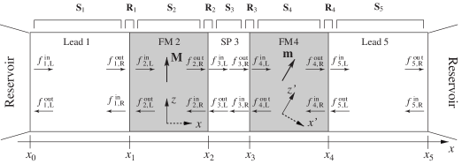
Figure 2: Scattering matrices. The center of the figure lists the incoming and outgoing distribution functions at each of the layers. The top lists the layer, $S_{n}$, and interface, $R_{n}$ scattering matrices that relate the distribution functions.

The eigensolutions are used to construct a scattering matrix which relates the boundary values of each layer. Figure 2 shows a schematic picture of a spin valve, where lead/FM/spacer/FM/lead are labeled layer 1 to layer 5, and $x_{0,1,2,3,4,5}$ denotes the $x$ coordinate of each interface. In Eq. (LABEL:eqn:FM-sol) and Eq. (20), we expand the distribution function in each layer using a set of eigensolutions. From these expansions we construct the (layer) scattering matrix for layer m, $\mathbb{S}_{m}$, which relates the incoming electron distribution functions $f_{\rm m,L/R}^{\rm in}$ and the outgoing ones $f_{\rm m,L/R}^{\rm out}$ at the left (L) and right (R) sides of the layer m (Figure 2):

$$\left[\begin{array}[]{c}f_{\rm m,L}^{\rm out}\\ f_{\rm m,R}^{\rm out}\end{array}\right]=\mathbb{S}_{m}\left[\begin{array}[]{c}f_{\rm m,L}^{\rm in}\\ f_{\rm m,R}^{\rm in}\end{array}\right].$$ (21)

Here, the matrices in the ferromagnet ($m=$ 2, 4) and non-magnet($m=$ 1, 3, 5) are respectively

$$\left[f_{\rm m,L}^{\rm in}\right]^{\rm T} = \left[f_{\rm m,L}^{\rm in,\uparrow},f_{\rm m,L}^{\rm in,\downarrow}\right]$$

$$\left[f_{\rm m,L}^{\rm in}\right]^{\rm T} = \left[f_{\rm m,L}^{\rm in,0},f_{\rm m,L}^{\rm in,x},f_{\rm m,L}^{\rm in,y},f_{\rm m,L}^{\rm in,z}\right].$$ (22)

and $f_{\rm m,L}^{\rm in,\uparrow}=f_{\rm m}^{\uparrow}(x_{m-1},{\bf k}_{i}^{+})$, and $f_{\rm m,R}^{\rm in,\uparrow}=f_{\rm m}^{\uparrow}(x_{m},{\bf k}_{i}^{-})$, etc. ${\bf k}_{i}^{\pm}$ is the electrons’ wave-vector on the Fermi surface with the (+/-) superscript indicating whether the electorn is right (+) or left (-) going. The superscripts “in” and “out” denote electrons going into or out of the layer. The definition in Eq. (22) generalizes in a straightforward manner for “R” and “out.”

From Eq. (LABEL:eqn:FM-sol), we can express the distribution function as $f_{\rm m}^{\sigma}(x,{\bf k}_{i})=\vec{F}^{\sigma}(x,{\bf k}_{i})\cdot\vec{\alpha}^{s}$ in the ferromagnetic layers (m = 2, 4), then

$$\left[\begin{array}[]{c}f_{\rm m,L}^{\rm out}\\ f_{\rm m,R}^{\rm out}\end{array}\right] = \left[\begin{array}[]{c}\vec{F}^{\uparrow}(x_{m-1},{\bf k}_{i}^{-})\\ \vec{F}^{\downarrow}(x_{m-1},{\bf k}_{i}^{-})\\ \vec{F}^{\uparrow}(x_{m},{\bf k}_{i}^{+})\\ \vec{F}^{\downarrow}(x_{m},{\bf k}_{i}^{+})\end{array}\right]\cdot\vec{\alpha}\equiv\vec{\bf F}_{m}^{\rm out}\cdot\vec{\alpha}$$ (29)

$$\left[\begin{array}[]{c}f_{\rm m,L}^{\rm in}\\ f_{\rm m,R}^{\rm in}\end{array}\right] = \left[\begin{array}[]{c}\vec{F}^{\uparrow}(x_{m-1},{\bf k}_{i}^{+})\\ \vec{F}^{\downarrow}(x_{m-1},{\bf k}_{i}^{+})\\ \vec{F}^{\uparrow}(x_{m},{\bf k}_{i}^{-})\\ \vec{F}^{\downarrow}(x_{m},{\bf k}_{i}^{-})\end{array}\right]\cdot\vec{\alpha}\equiv\vec{\bf F}_{m}^{\rm in}\cdot\vec{\alpha},$$ (36)

where $\vec{\bf F}_{m}^{\rm in}$ and $\vec{\bf F}_{m}^{\rm out}$ are both $2N\times 2N$ square matrices. Therefore, Eq. (21) implies that the layer scattering matrix for ferromagnetic layers (m = 2, 4) is

$$\mathbb{S}_{m}=\vec{\bf F}_{m}^{\rm out}\cdot\left[\vec{\bf F}_{m}^{\rm in}\right]^{-1}.$$ (37)

The layer scattering matrix for non-magnetic layers (m = 1, 3, 5) is constructed in a similar way using Eq. (20) as the expansion and Eq. (22) for m = 1, 3, 5.

3.4 Interface scattering matrix

Using the layer scattering matrix, we are able to relate the distribution function values at the two sides of a bulk layer. Next, we find an interface scattering matrix which connects the distribution functions across an interface. Right at the interface, the Boltzmann equation is not valid because the material properties vary rapidly. The distribution functions across the interface are related through the scattering matrix for the electron wave-functions at the interface.

Like the layer scattering matrix in Eq. (21), the interface scattering matrix $\mathbb{R}$ relates the incoming to the outgoing distribution functions. If the interface is specular, when electrons scatter from the interface, the component of the wave vector that is parallel to the interface is conserved. In this case, the interface scattering matrix is block diagonal, with non-zero elements only for those states with the same parallel wave vector. On the other hand, defect scattering at the interface couples states with different parallel wave vectors and the interface scattering matrix becomes dense. In the present work, we neglect defect scattering at the interfaces for simplicity. Interfacial defect scattering has been considered by several authors Dugaev:1995 ; Zhang:1996 ; Xia:2006 . Xia et al. Xia:2006 treated interdiffusion at Co/Cu interfaces with first principles calculations and found that such defects caused only minor changes in the average transport properties for these interfaces.

Consider an isolated interface between a non-magnet and a ferromagnet (NM/FM) and choose the spin quantization axis to be parallel to the magnetization of the ferromagnet. The interface between Lead 1 and FM2 in Figure 2 is such an interface if those two materials were extended to infinity. Suppose the wave-function for an electron on the Fermi surface in the corresponding NM is $\phi({\bf k}_{i})$, which is orthonormal to other states on the Fermi surface: $\langle\phi({\bf k}_{i})|\phi({\bf k}_{j})\rangle=\delta_{ij}$. The wave-function for an electron on the Fermi surface in the FM is $\psi_{\sigma}({\bf k}_{i})$, which is also orthonormal to other states on the Fermi surface: $\langle\psi_{\sigma}({\bf k}_{i})|\psi_{\sigma^{\prime}}({\bf k}_{j})\rangle=\delta_{ij}\delta_{\sigma\sigma^{\prime}}$.

In the non-magnet, the wave-function for an electron moving toward the interface with spin pointing in an arbitrary direction is written as a linear combination of spin-up and spin-down components:

$$\Phi_{\rm in}=\left[\begin{array}[c]{c}a\phi({\bf k}_{i}^{+})\\ b\phi({\bf k}_{i}^{+})\end{array}\right],$$ (38)

where $a$ and $b$ are the coefficients of the up and down spinor components. This incident state is scattered at the NM/FM interface, and the scattered states are

$$\Phi_{\rm ref} = \sum_{j}\left[\begin{array}[c]{c}aR^{\rm NN,\uparrow}_{ij}\phi({\bf k}_{j}^{-})\\ bR^{\rm NN,\downarrow}_{ij}\phi({\bf k}_{j}^{-})\end{array}\right]\quad\mbox{for}\quad x<0,$$ (41)

$$\Phi_{\rm tr} = \sum_{j}\left[\begin{array}[c]{c}aT^{\rm NF,\uparrow}_{ij}\psi_{\uparrow}({\bf k}_{j}^{+})\\ bT^{\rm NF,\downarrow}_{ij}\psi_{\downarrow}({\bf k}_{j}^{+})\end{array}\right]\quad\mbox{for}\quad x>0,$$ (44)

where $R^{\rm NN,\sigma}_{ij}$ and $T^{\rm NF,\sigma}_{ij}$ are the reflection and transmission amplitudes for electron from ${\bf k}_{i}$ to ${\bf k}_{j}$ for spin-up and spin-down electrons: $\sigma=\uparrow,\downarrow$.

The $2\times 2$ matrix distribution function is then defined by the outer product of the spinor coefficients. For instance, for the incident state

$$\hat{f}_{\rm in}=\left[\begin{array}[c]{cc}aa^{*}&ab^{*}\\ ba^{*}&bb^{*}\end{array}\right].$$ (45)

Straightforward algebra reveals

$$\hat{f}_{\rm ref}({\bf k}_{j}^{-}) = {\mathbf{R}_{ij}^{\rm NN}}^{\dagger}\hat{f}_{\rm in}({\bf k}_{i}^{+})\mathbf{R}_{ij}^{\rm NN}$$

$$\hat{f}_{\rm tr}({\bf k}_{j}^{+}) = {\mathbf{T}_{ij}^{\rm NF}}^{\dagger}\hat{f}_{\rm in}({\bf k}_{i}^{+})\mathbf{T}_{ij}^{\rm NF},$$ (46)

where the reflection matrix (NM to NM) and transmission matrix (NM to FM) are

$$\mathbf{R}_{ij}^{\rm NN} = \left[\begin{array}[c]{cc}R^{\rm NN,\uparrow}_{ij}&0\\ 0&R^{\rm NN,\downarrow}_{ij}\end{array}\right]$$ (49)

$$\mathbf{T}_{ij}^{\rm NF} = \left[\begin{array}[c]{cc}T^{\rm NF,\uparrow}_{ij}&0\\ 0&T^{\rm NF,\downarrow}_{ij}\end{array}\right].$$ (52)

Considering the electrons incident onto the interface from both sides of the interface, the scattering relationship Eq. (46) becomes

$$\hat{f}_{\rm N}({\bf k}_{j}^{-}) =\sum_{i}{\mathbf{R}_{ij}^{\rm NN}}^{\dagger}\hat{f}_{\rm N}({\bf k}_{i}^{+})\mathbf{R}_{ij}^{\rm NN}+\sum_{i}{\mathbf{T}_{ij}^{\rm FN}}^{\dagger}\hat{f}_{\rm F}({\bf k}_{i}^{-})\mathbf{T}_{ij}^{\rm FN},$$ (53a)

$$\hat{f}_{\rm F}({\bf k}_{j}^{+}) =\sum_{i}{\mathbf{R}_{ij}^{\rm FF}}^{\dagger}\hat{f}_{\rm F}({\bf k}_{i}^{-})\mathbf{R}_{ij}^{\rm FF}+\sum_{i}{\mathbf{T}_{ij}^{\rm NF}}^{\dagger}\hat{f}_{\rm N}({\bf k}_{i}^{+})\mathbf{T}_{ij}^{\rm NF}.$$ (53b)

The matrix forms of the distribution functions $\hat{f}$ in Eq. (53) are expanded using $\sigma_{\uparrow,\downarrow}$ in the FM or Pauli matrices $\sigma_{0,x,y,z}$ in the NM as in Eq. (8). We represent the distribution functions by their expansion components $f_{\uparrow,\downarrow}$ in the FM and $f_{0,x,y,z}$ in the NM as in Eq. (22). After this transformation, the scattering formula Eq. (53) is written as

$$\left[\begin{array}[]{c}f_{\rm N}^{\rm in}\\ f_{\rm F}^{\rm in}\end{array}\right]\equiv\left[\begin{array}[]{c}f_{\rm N}^{0}(x_{0},{\bf k}_{i}^{-})\\ f_{\rm N}^{x}(x_{0},{\bf k}_{i}^{-})\\ f_{\rm N}^{y}(x_{0},{\bf k}_{i}^{-})\\ f_{\rm N}^{z}(x_{0},{\bf k}_{i}^{-})\\ f_{\rm F}^{\uparrow}(x_{0},{\bf k}_{i}^{+})\\ f_{\rm F}^{\downarrow}(x_{0},{\bf k}_{i}^{+})\end{array}\right]=\mathbb{R}\left[\begin{array}[]{c}f_{\rm N}^{0}(x_{0},{\bf k}_{i}^{+})\\ f_{\rm N}^{x}(x_{0},{\bf k}_{i}^{+})\\ f_{\rm N}^{y}(x_{0},{\bf k}_{i}^{+})\\ f_{\rm N}^{z}(x_{0},{\bf k}_{i}^{+})\\ f_{\rm F}^{\uparrow}(x_{0},{\bf k}_{i}^{-})\\ f_{\rm F}^{\downarrow}(x_{0},{\bf k}_{i}^{-})\end{array}\right]\equiv\mathbb{R}\left[\begin{array}[]{c}f_{\rm N}^{\rm out}\\ f_{\rm F}^{\rm out}\end{array}\right],$$ (54)

where $\mathbb{R}$ is the interface scattering matrix for the distribution functions across the interface, and the matrix elements in $\mathbb{R}$ are obtained from the scattering matrices $\mathbf{R}$ and $\mathbf{T}$ in Eq. (52). Note the apparent reversal of “in” and “out” in Eq. (54) compared to that in in Eq. (21). The directions in and out are defined with respect to the layers, rather than the interfaces and the incoming distribution for one of the layers is the outgoing distribution for one of the interfaces.

3.5 System scattering matrix

With all the layer and interface scattering matrices $\mathbb{S}_{1,2,3,4,5}$ and $\mathbb{R}_{1,2,3,4}$ (see Figure 2), we are ready to construct a system-wide scattering matrix ${\mathbb{T}}$ that relates the incoming and outgoing distribution functions near the left and right reservoirs. The scattering matrix ${\mathbb{T}}$ is obtained by joining all the layer scattering matrices and interface scattering matrices in order: $\mathbb{T}=\mathbb{S}_{1}-\mathbb{R}_{1}-\mathbb{S}_{2}-\mathbb{R}_{2}-\mathbb{S}_{3}-\mathbb{R}_{3}-\mathbb{S}_{4}-\mathbb{R}_{4}-\mathbb{S}_{5}$.

The joining procedure is as follows. First we join $\mathbb{S}_{1}$ to $\mathbb{R}_{1}$ (see Figure 2), where $\mathbb{S}_{1}$ is the layer scattering matrix that covers the interval $[x_{0}^{+},x_{1}^{-}]$ (layer 1), and $\mathbb{R}_{1}$ is the interface scattering matrix that covers $[x_{1}^{-},x_{1}^{+}$] (the interface at $x_{1}$):

$$\left[\begin{array}[]{c}f_{\rm 1,L}^{\rm out}\\ f_{\rm 1,R}^{\rm out}\end{array}\right] = \left[\begin{array}[]{cc}\mathbb{S}_{1}^{\rm LL}&\mathbb{S}_{1}^{\rm LR}\\ \mathbb{S}_{1}^{\rm RL}&\mathbb{S}_{1}^{\rm Rb}\end{array}\right]\left[\begin{array}[]{c}f_{\rm 1,L}^{\rm in}\\ f_{\rm 1,R}^{\rm in}\end{array}\right]$$ (61)

$$\left[\begin{array}[]{c}f_{\rm 1,R}^{\rm in}\\ f_{\rm 2,L}^{\rm in}\end{array}\right] = \left[\begin{array}[]{cc}\mathbb{R}_{1}^{\rm LL}&\mathbb{R}_{1}^{\rm LR}\\ \mathbb{R}_{1}^{\rm RL}&\mathbb{R}_{1}^{\rm Rb}\end{array}\right]\left[\begin{array}[]{c}f_{\rm 1,R}^{\rm out}\\ f_{\rm 2,L}^{\rm out}\end{array}\right].$$ (68)

Here we have subdivided the distribution vectors (discretized functions) into two subvectors for the values on the left (L) and right (R). The $\mathbb{S}$ and $\mathbb{R}$ matrices are correspondingly subdivided into four submatrices labelled LL, LR, RL, and RR, where, for example, the LR submatrix connects incoming values on the right to outgoing values on the left. We denote the joint scattering matrix by $\mathbb{T}_{\rm li}$, where the subscript “l” denotes a lead, “i” denotes an NM/FM or FM/NM interface, “f” denotes a ferromagnet, and “n” denotes the non-magnetic spacer layer. $\mathbb{T}_{\rm li}$ covers $[x_{0}^{+},x_{1}^{+}]$ and relates $f_{\rm 1,L}^{\rm in/out}$ and $f_{\rm 2,L}^{\rm in/out}$:

$$\left[\begin{array}[]{c}f_{\rm 1,L}^{\rm out}\\ f_{\rm 2,L}^{\rm in}\end{array}\right]=\mathbb{T}_{\rm li}\left[\begin{array}[]{c}f_{\rm 1,L}^{\rm in}\\ f_{\rm 2,L}^{\rm out}\end{array}\right].$$ (69)

By eliminating the intermediate distribution functions $f_{\rm 1,R}^{\rm in/out}$ in Eq. (68), we have

$$\mathbb{T}_{\rm li}=\left[\begin{array}[]{cc}\mathbb{T}^{\rm LL}&\mathbb{T}^{\rm LR}\\ \mathbb{T}^{\rm RL}&\mathbb{T}^{\rm RR}\end{array}\right],$$ (70)

where

$$\mathbb{T}^{\rm LL} = \mathbb{S}_{1}^{\rm LL}+\mathbb{S}_{1}^{\rm LR}\mathbb{R}_{1}^{\rm LL}(1-\mathbb{S}_{1}^{\rm RR}\mathbb{R}_{1}^{\rm LL})^{-1}\mathbb{S}_{1}^{\rm RL}$$

$$\mathbb{T}^{\rm LR} = \mathbb{S}_{1}^{\rm LR}[1+\mathbb{R}_{1}^{\rm LL}(1-\mathbb{S}_{1}^{\rm RR}\mathbb{R}_{1}^{\rm LL})^{-1}\mathbb{S}_{1}^{\rm RR}]\mathbb{R}_{1}^{\rm LR}$$

$$\mathbb{T}^{\rm RL} = \mathbb{R}_{1}^{\rm RL}(1-\mathbb{S}_{1}^{\rm RR}\mathbb{R}_{1}^{\rm LL})^{-1}\mathbb{S}_{1}^{\rm RL}$$

$$\mathbb{T}^{\rm RR} = \mathbb{R}_{1}^{\rm RR}+\mathbb{R}_{1}^{\rm RL}(1-\mathbb{S}_{1}^{\rm RR}\mathbb{R}_{1}^{\rm LL})^{-1}\mathbb{S}_{1}^{\rm RR}\mathbb{R}_{1}^{\rm LR}.$$ (71)

The scattering matrices described here and the method of joining them is more complicated than approaches using transfer matrices, which relate the boundary values from one side to the other rather than outgoing to incoming boundary values. However, transfer matrix approaches become unstable as layers become thick and the present method does not.

Using the same procedure as above we can join $\mathbb{T}_{\rm li}$ with $\mathbb{S}_{2}$ and then with $\mathbb{R}_{2}$ to have a scattering matrix $\mathbb{T}_{\rm lifi}$ which covers $[x_{0}^{+},x_{2}^{+}]$. We continue to construct $\mathbb{T}_{\rm lif}$, $\mathbb{T}_{\rm lifi}$, $\mathbb{T}_{\rm lifin}$, $\mathbb{T}_{\rm lifini}$, $\mathbb{T}_{\rm lifinif}$, $\mathbb{T}_{\rm lifinifi}$, and $\mathbb{T}_{\rm lifinifil}$. When coming to the the spacer layer, the eigensolutions and the scattering matrix $\mathbb{S}_{3}$ use $z^{\prime}$-axis instead of the $z$-axis (which is used for $\mathbb{T}_{\rm lifi}$) as the spin quantization axis (see Figure 2). Therefore, we have to make an axis rotation at the spacer layer when joining $\mathbb{T}_{\rm lifi}$ with $\mathbb{S}_{3}$.

The distribution functions that $\mathbb{T}_{\rm lifi}$ and $\mathbb{S}_{3}$ relate are:

$$\left[\begin{array}[]{c}f_{\rm 1,L}^{\rm out}\\ f_{\rm 3,L}^{\rm in}\end{array}\right] = \mathbb{T}_{\rm lifi}\left[\begin{array}[]{c}f_{\rm 1,L}^{\rm in}\\ f_{\rm 3,L}^{\rm out}\end{array}\right]$$ (76)

$$\left[\begin{array}[]{c}f_{\rm 3,L}^{\rm out^{\prime}}\\ f_{\rm 3,R}^{\rm out^{\prime}}\end{array}\right] = \mathbb{S}_{3}\left[\begin{array}[]{c}f_{\rm 3,L}^{\rm in^{\prime}}\\ f_{\rm 3,R}^{\rm in^{\prime}}\end{array}\right],$$ (81)

The primed distribution functions are written using the $z^{\prime}$-axis as the spin quantization axis. To join $\mathbb{T}_{\rm lifi}$ with $\mathbb{S}_{3}$, we write $f_{\rm 3,L}^{\rm in/out}$ in terms of $f_{\rm 3,L}^{\rm in/out^{\prime}}$: $f_{\rm 3,L}^{\rm in/out}=\hat{}\mathbf{U}^{\dagger}f_{\rm 3,L}^{\rm in/out^{\prime}}$. $\hat{}\mathbf{U}$ is the component representation [Eq. (22)] of the unitary rotation matrix $\hat{U}$ in Eq. (8): $\hat{f}^{\prime}=\hat{U}\hat{f}\hat{U}^{\dagger}\Rightarrow f^{\prime}=\hat{}\mathbf{U}f$. Then

$$\left[\begin{array}[]{c}f_{\rm 1,L}^{\rm out}\\ \hat{}\mathbf{U}^{\dagger}f_{\rm 3,L}^{\rm in^{\prime}}\end{array}\right]=\mathbb{T}_{\rm lifi}\left[\begin{array}[]{c}f_{\rm 1,L}^{\rm in}\\ \hat{}\mathbf{U}^{\dagger}f_{\rm 3,L}^{\rm out^{\prime}}\end{array}\right]\Longrightarrow\left[\begin{array}[]{c}f_{\rm 1,L}^{\rm out}\\ f_{\rm 3,L}^{\rm in^{\prime}}\end{array}\right]=\mathbb{T}_{\rm lifi}^{\prime}\left[\begin{array}[]{c}f_{\rm 1,L}^{\rm in}\\ f_{\rm 3,L}^{\rm out^{\prime}}\end{array}\right],$$ (82)

with the rotated scattering matrix

$$\mathbb{T}_{\rm lifi}^{\prime}=\left[\begin{array}[]{cc}1&0\\ 0&\hat{}\mathbf{U}\end{array}\right]\mathbb{T}_{\rm lifi}\left[\begin{array}[]{cc}1&0\\ 0&\hat{}\mathbf{U}^{\dagger}\end{array}\right].$$ (83)

$\mathbb{T}_{\rm lifi}^{\prime}$ is joined with $\mathbb{S}_{3}$ using the same procedure as in Eq. (70) and becomes $\mathbb{T}_{\rm lifin}$. Continuing by joining $\mathbb{T}_{\rm lifin}$ to $\mathbb{R}_{3},\mathbb{S}_{4},\mathbb{R}_{4}$ and $\mathbb{S}_{5}$ gives a system wide scattering matrix $\mathbb{T}=\mathbb{T}_{\rm lifinifil}$ that relates the distribution functions near the left reservoir and the right reservoir:

$$\left[\begin{array}[]{c}f_{1}(x_{0},{\bf k}_{i}^{-})\\ f_{5}^{\prime}(x_{5},{\bf k}_{i}^{+})\end{array}\right]\equiv\left[\begin{array}[]{c}f_{\rm 1,L}^{\rm out}\\ f_{\rm 5,R}^{\rm out^{\prime}}\end{array}\right]=\mathbb{T}\left[\begin{array}[]{c}f_{\rm 1,L}^{\rm in}\\ f_{\rm 5,R}^{\rm in^{\prime}}\end{array}\right]\equiv\mathbb{T}\left[\begin{array}[]{c}f_{1}(x_{0},{\bf k}_{i}^{+})\\ f_{5}^{\prime}(x_{5},{\bf k}_{i}^{-})\end{array}\right].$$ (84)

Eq. (84) is a condition on the boundary values of the distribution functions for an arbitrary solution of the Boltzmann equation in the multilayer.

In the case that the two leads (layer 1 and layer 5) are semi-infinite, we need a system scattering matrix $\mathbb{T}$ that covers the interval $[x_{1}^{-},x_{4}^{+}]$:

$$\left[\begin{array}[]{c}f_{1}(x_{1},{\bf k}_{i}^{-})\\ f_{5}^{\prime}(x_{4},{\bf k}_{i}^{+})\end{array}\right]=\mathbb{T}\left[\begin{array}[]{c}f_{1}(x_{1},{\bf k}_{i}^{+})\\ f_{5}^{\prime}(x_{4},{\bf k}_{i}^{-})\end{array}\right].$$ (85)

Eq. (84) and Eq. (85) each have a total of $8N$ unknown coefficients in the expansions of $f_{1}$ and $f_{5}$ but only $4N$ equations. To solve this problem, we study the boundary conditions, which apply restrictions on the distribution functions $f_{1}$ and $f_{5}$, and so reduce the number of unknowns in the expansions.

3.6 Boundary conditions

By examining the properties of the leads and reservoirs, we can restrict the form of the distribution functions $f_{1}$ and $f_{5}$ in the leads, such that the number of unknown coefficients in the expansions equals the number of equations in Eq. (84) or Eq. (85). Thus, we can uniquely determine the distribution functions from Eq. (84) and Eq. (85). We treat semi-infinite leads and finite leads differently, and separate the discussion into two cases: 1) the leads are semi-infinite: the left/right lead extends to the left/right infinitely, and 2) both leads have finite length before connecting to reservoirs.

3.6.1 Semi-infinite leads

If the leads are semi-infinite, the distribution function $f_{1}$ in the left lead (layer 1) includes only the exponential eigensolutions with $\lambda_{n}>0$. Then from Eq. (20), we have

$$f_{1}^{0}(x,{\bf k}_{i}) =\alpha_{1}^{0}F_{1}^{0}(x,{\bf k}_{i})+F_{2}^{0}(x,{\bf k}_{i})+\mathop{\sum_{n=3}^{N}}_{\lambda_{n}>0}\alpha_{n}^{0}F_{n}^{0}(x,{\bf k}_{i}),$$ (86a)

$$f_{1}^{x,y,z}(x,{\bf k}_{i}) =\mathop{\sum_{n=1}^{N}}_{\lambda_{n+N}>0}\alpha_{n}^{x,y,z}F_{n}^{x,y,z}(x,{\bf k}_{i}).$$ (86b)

We set $\alpha_{2}^{0}=1$ to fix the current, because $F_{2}$ is the current carrying term. Due to the $x$-translational invariance of the exponential eigensolutions, half of the eigenvalues $\lambda_{n}$ are positive and half are negative for charge transport and spin transport, respectively. Therefore there are $2N$ unknown $\alpha_{n}^{0,x,y,z}$ in total, $N/2$ for each component of $0,x,y$, and $z$.

Similarly, the distribution function $f_{5}^{\prime}$ in the right lead (layer 5) includes only the exponential eigensolutions with $\lambda_{n}<0$:

$${f_{5}^{\prime}}^{0}(x,{\bf k}_{i}) =\beta_{2}^{0}F_{2}^{0}(x,{\bf k}_{i})+\mathop{\sum_{n=3}^{N}}_{\lambda_{n}<0}\beta_{n}^{0}F_{n}^{0}(x,{\bf k}_{i}),$$ (87a)

$${f_{5}^{\prime}}^{\tau}(x,{\bf k}_{i}) =\mathop{\sum_{n=1}^{N}}_{\lambda_{n+N}<0}\beta_{n}^{\tau}F_{n}^{\tau}(x,{\bf k}_{i}).$$ (87b)

where $\tau=x,y,z$. The choice $\beta_{1}^{0}=0$ sets the potential at the right lead to be zero. Eq. (87) also has $2N$ unknowns, $\beta_{n}^{\tau}$, $\tau=0,x,y,z$, in total.

Plugging Eq. (86) and Eq. (87) into Eq. (85), we have $4N$ equations with $4N$ unknowns, the expansion coefficients $\alpha_{n}$’s and $\beta_{n}$’s can be solved. This gives the distribution functions in the left and right leads. The distribution function values inside the spin valve are calculated from the boundary values using the appropriate scattering matrices, as will be shown later.

3.6.2 Finite leads

In actual spin valve samples, the leads are usually short, after which the sample connects to essentially bulk material, here referred to as reservoirs. Electrons that enter the reservoir are much less likely to scatter back into the sample than to stay in the reservoir until they are thermalized. This means that the reservoirs behave as perfect absorbers. The distribution of the electrons coming out of the reservoir is characteristic of the bulk, independent of the distribution of electrons coming in. The connection between the reservoirs and leads has been studied in more detail by Berger Berger:2004 and Hamerle et al. Hamrle:2005 . When the leads have finite length and are connected to electron reservoirs, the exponential eigensolutions have no singularities and all of them should be included. In such a case, the form of the distribution functions is constrained by the following properties of a reservoir: the electrons leaving the reservoir have a bulk-like distribution function and the electrons with arbitrary distribution function can be absorbed by the reservoir. Based on these two properties of reservoirs, we propose that the distribution function near the reservoirs should satisfy: (1) for the electrons going from the reservoir to the lead, the distribution function is bulk-like, namely $f_{\rm 1,L}^{\rm in}$ and $f_{\rm 5,R}^{\rm in^{\prime}}$ are spin independent and have contributions only from $F_{1}^{0}$ and $F_{2}^{0}$ in Eq. (19); (2) for the electrons going from the lead to the reservoir, the distribution function has whatever structure it wishes, namely $f_{\rm 1,L}^{\rm out}$ and $f_{\rm 5,R}^{\rm out^{\prime}}$ have contributions from all $F_{n}^{0,x,y,z}$.

To determine the form of the distribution functions near the reservoirs, let us first use $F_{p}^{0,x,y,z}$ to denote the eigensolutions with positive eigenvalues: $\lambda_{p}>0$; and use $F_{q}^{0,x,y,z}$ to denote the eigensolutions with negative eigenvalues: $\lambda_{q}<0$. We construct a new set of basis functions $G_{n}^{0,x,y,z}$ using linear combinations of the old basis functions $F_{n}^{0,x,y,z}$ such that,

$$G_{1,2}^{0,x,y,z} =F_{1,2}^{0,x,y,z},$$ (88a)

$$G_{p}^{0,x,y,z}(x_{0},{\bf k}_{i}^{+}) =0,$$ (88b)

$$G_{q}^{0,x,y,z}(x_{5},{\bf k}_{i}^{-}) =0.$$ (88c)

Essentially, $G_{p}$ is obtained by using the linear combination of $F_{1}(x_{0},{\bf k}_{i}^{+})$ and $F_{q}(x_{0},{\bf k}_{i}^{+})$ to cancel $F_{p}(x_{0},{\bf k}_{i}^{+})$, and similarly $G_{q}$ is obtained by using $F_{1}(x_{5},{\bf k}_{i}^{-})$ and $F_{p}(x_{5},{\bf k}_{i}^{-})$ to cancel $F_{q}(x_{5},{\bf k}_{i}^{-})$.

$G_{1,2}$ and $G_{p}$ form the basis for the electrons that have bulk-like right-going behavior at $x=x_{0}$, and $G_{1,2}$ and $G_{q}$ form the basis for electrons that have bulk-like left-going behavior at $x=x_{5}$. The distribution functions that satisfy the requirements (1) and (2) in the leads are constructed as the following:

$$f_{1}^{0}(x,{\bf k}_{i}) =\alpha_{1}^{0}G^{0}_{1}(x,{\bf k}_{i})+G^{0}_{2}(x,{\bf k}_{i})+\sum_{p}\alpha_{p}^{0}G^{0}_{p}(x,{\bf k}_{i}),$$ (89a)

$$f_{1}^{x,y,z}(x,{\bf k}_{i}) =\sum_{p}\alpha_{p}^{x,y,z}G^{x,y,z}_{p}(x,{\bf k}_{i}),$$ (89b)

$${f^{\prime}}_{5}^{0}(x,{\bf k}_{i}) =\beta_{2}^{0}G^{0}_{2}(x,{\bf k}_{i})+\sum_{q}\beta_{q}^{0}G^{0}_{q}(x,{\bf k}_{i}),$$ (89c)

$${f^{\prime}}_{5}^{x,y,z}(x,{\bf k}_{i}) =\sum_{q}\beta_{q}^{x,y,z}G^{x,y,z}_{q}(x,{\bf k}_{i}).$$ (89d)

In these equations, $\alpha_{2}^{0}=1$ fixes the current, and $\beta_{1}^{0}=0$ fixes the chemical potential at the right boundary to be zero. Since the indexes $p$ and $q$ each take $(N-2)/2$ values for the 0-component and $N/2$ values for the $\{x,y,z\}$-components, the total number of unknown coefficients in Eq. (89) is $4N$. Therefore, by plugging Eq. (89) into Eq. (84), the coefficients $\alpha_{n}^{s},\beta_{n}^{s}$ can be determined.

3.7 System distribution function

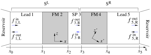
Figure 3: Back-propagation matrices.

Once we have the distribution function values at the boundaries, either near the lead/FM interface for the semi-infinite lead case or near the reservoir for the finite lead case, we can calculate the distribution function values everywhere inside the spin valve using the scattering matrices. For example, assume the scattering matrices $\mathbb{S}^{L}$ covers the interval $[x_{0}^{+},x_{3}^{-}]$ and $\mathbb{S}^{R}$ covers the interval $[x_{3}^{-},x_{5}^{-}]$:

$$\left[\begin{array}[]{c}f_{\rm 1,L}^{\rm out}\\ f_{\rm 3,R}^{\rm out^{\prime}}\end{array}\right] = \left[\begin{array}[]{cc}\mathbb{S}^{L}_{\rm LL}&\mathbb{S}^{L}_{\rm LR}\\ \mathbb{S}^{L}_{\rm RL}&\mathbb{S}^{L}_{\rm RR}\end{array}\right]\left[\begin{array}[]{c}f_{\rm 1,L}^{\rm in}\\ f_{\rm 3,R}^{\rm in^{\prime}}\end{array}\right]$$ (96)

$$\left[\begin{array}[]{c}f_{\rm 3,R}^{\rm in^{\prime}}\\ f_{\rm 5,R}^{\rm out^{\prime}}\end{array}\right] = \left[\begin{array}[]{cc}\mathbb{S}^{R}_{\rm LL}&\mathbb{S}^{R}_{\rm LR}\\ \mathbb{S}^{R}_{\rm RL}&\mathbb{S}^{R}_{\rm RR}\end{array}\right]\left[\begin{array}[]{c}f_{\rm 3,R}^{\rm out^{\prime}}\\ f_{\rm 5,R}^{\rm in^{\prime}}\end{array}\right].$$ (103)

$f_{\rm 3,R}^{\rm in/out^{\prime}}$ can be solved from Eq. (103), but the equations in Eq. (103) are redundant, so we choose the half of the equations that use the incoming boundary values rather than the outgoing ones, i.e.,

$$f_{\rm 3,R}^{\rm out^{\prime}} =\mathbb{S}^{L}_{\rm RL}f_{\rm 1,L}^{\rm in}+\mathbb{S}^{L}_{\rm RR}f_{3,R}^{\rm in^{\prime}},$$ (104a)

$$f_{\rm 3,R}^{\rm in^{\prime}} =\mathbb{S}^{R}_{\rm LL}f_{\rm 3,R}^{\rm out^{\prime}}+\mathbb{S}^{R}_{\rm LR}f_{5,R}^{\rm in^{\prime}}.$$ (104b)

From these equations, we can calculate $f_{\rm 3,R}^{\rm in/out^{\prime}}$. Similarly, we can calculate the distribution function value elsewhere using a different pair of scattering matrices $\mathbb{S}^{L}$ and $\mathbb{S}^{R}$.

3.8 Transport properties

With the distribution functions in hand, it is straightforward to calculate transport properties $h(\bf k)$ by integrating over the whole Fermi surface:

$$h=\int_{\rm FS}h({\bf k})d\vec{k}`.$$ (105)

Using Eq. (9), the integrations for spin density and spin current are discretized as

$$\mbox{spin density:}\qquad n_{m}^{s}(x) =\sum_{i=1}^{N}w_{i}f^{s}_{m}(x,{\bf k}_{i}),$$ (106a)

$$\mbox{spin current:}\qquad\vec{j}_{m}^{s}(x) =\sum_{i=1}^{N}w_{i}{\bf v}_{i}f^{s}_{m}(x,{\bf k}_{i}),$$ (106b)

where $s=0,x,y,z$ for $m=1,3,5$ (non-magnetic layers), and $s=\uparrow,\downarrow$ for $m=2,4$ (ferromagnetic layers). The spin current at $x=x_{3}^{-}$ is written in the $x^{\prime}$-$z^{\prime}$ frame:

$${\bf Q}(x_{3}^{-})=j_{3}^{x}(x_{3}^{-})\hat{\bf x}^{\prime}+j_{3}^{z}(x_{3}^{-})\hat{\bf z}^{\prime},$$ (107)

where the $j_{3}^{z}(x_{3}^{-})$ is the longitudinal piece parallel to the right FM layer’s magnetization ($z^{\prime}$ direction), and $j_{3}^{x}(x_{3}^{-})$ is the piece perpendicular to $z^{\prime}$-axis. From Ref. Stiles:2002b we know that the perpendicular spin current is absorbed at the NM/FM interface, therefore the spin-transfer torque acting on the right FM layer is

$${\bf N}_{\rm st}=j_{3}^{x}(x_{3}^{-})\hat{\bf x}^{\prime}.$$ (108)

4 Applications

In this section, we apply our numerical method to calculate the spin-transfer torque acting on the right ferromagnetic layer of a model spin valve. We compare the results with equivalent calculations using the drift-diffusion approach and Slonczewski’s hybrid theory. First, we describe the approximations we make to simplify the calculation so as to focus on the differences between the different approaches.

4.1 Approximations and their rationale

Compared with the drift-diffusion method and circuit theory, the most important feature of the Boltzmann method is its treatment of electrons in the bulk moving in different directions. In circuit theory, the average over the Fermi surface, the spin accumulation, is used to characterize the electrons inside that node (here a layer). In this treatment all of the electrons inside a node are effectively aligned. In the drift diffusion approximation, the distribution is modeled by its first moment, the spin accumulation, and second moment with respect to velocity, the spin current. This allows for greater flexibility in describing the distribution function, but clearly if higher moments are important, neglecting them will lead to errors. In a Boltzmann equation treatment of the transport the distribution function is allowed its full flexibility.

To study the different approaches we consider a simple model in which we ignore the actual shape and/or size of the Fermi surfaces and assume that the Fermi surfaces in both the non-magnet and the ferromagnet (both spin-up and spin-down) are perfectly spherical and are the same size. We use different mean free paths to distinguish the differences between the electrons in the non-magnet and the ferromagnet: $l_{\rm N}$ for non-magnet, $l_{\rm F}^{\uparrow,\downarrow}$ for spin-up and spin-down electrons in ferromagnet. The choice of identical and spherical Fermi surfaces makes finding a wave vector mesh particularly simple. Since the problem is azimuthally symmetric, there are no contributions to the distribution function that are not azimuthally symmetric so that only polar variation need be considered. We choose Gauss-Legendre sampling for the polar direction with typically 40 mesh points.

For the interface scattering coefficients in Eq. (52), we treat the case of ideal interfaces with no defect scattering. Consider an electron with wave-vector $k_{x}$ incident on an interface. With the Fermi surface assumption made in the previous paragraph, the wave-vectors for the reflected and transmitted electrons are $-k_{x}$ and $k_{x}$, respectively. The matrix elements of the reflection and transmission matrices $\mathbf{R}$ and $\mathbf{T}$ in Eq. (52) are calculated in Ref. Stiles:2000 . To allow for finite and spin-dependent interface resistance in the equal-Fermi-surface model, we assume $\delta$-function scattering at the interface to give the following transmission and reflection probabilities:

$$|R_{ij}^{\rm NN,\sigma}|^{2}=|R_{ij}^{\rm FF,\sigma}|^{2} ={\alpha_{\sigma}\over\alpha_{\sigma}+(k_{i}^{x})^{2}}\delta_{k_{i}^{x},-k_{j}^{x}},$$ (109a)

$$|T_{ij}^{\rm NF,\sigma}|^{2}=|T_{ij}^{\rm FN,\sigma}|^{2} ={(k_{i}^{x})^{2}\over\alpha_{\sigma}+(k_{i}^{x})^{2}}\delta_{k_{i}^{x},k_{j}^{x}},$$ (109b)

where $\sigma=\uparrow$ or $\downarrow$, and $k_{i}^{x}$ is a discretization of $k_{x}$. The parameter $\alpha_{\sigma}$ is proportional to the square root of the strength of the $\delta$-function-like interface potential. This can be read off from the horizontal axis in Fig. 1 of Ref. Stiles:2000 using experimental spin dependent interface resistance data.

We also use the relaxation-time approximation: $P_{ij}^{\sigma}=P^{\sigma}=A_{\rm FS}/\tau_{\sigma}$ and $P_{ij}^{\rm sf}=P^{\rm sf}=A_{\rm FS}/\tau_{\rm sf}$, where $A_{\rm FS}$ is the area of the Fermi surface. In this limit, the current carrying eigensolution $F_{2}^{\sigma}$ in Eq. (17) reduces to $F_{2}^{\sigma}(x,{\bf k}_{i})=x+v_{i}^{x}l^{\sigma}/v_{F}$, where $l^{\sigma}$ is the mean free path for different spins and $v_{F}$ is the Fermi velocity.

Table 1: Material parameters used in the Boltzmann calculation.

Parameter	Material	Value	Units	Reference
$l$	Cu	110	nm	Stiles:2002a
$l_{\rm sf}$	Cu	450	nm	Bass:1999
$l^{\uparrow}$	Co	16.25	nm	Stiles:2002a
$l^{\downarrow}$	Co	6.01	nm	Stiles:2002a
$l_{\rm sf}$	Co	59	nm	Yang:1994
$\alpha_{\uparrow}$	Co/Cu	0.051		Stiles:2002a
$\alpha_{\downarrow}$	Co/Cu	0.393		Stiles:2002a

Using the algorithm described above in Sec. 2 and the approximations discussed above (equal, spherical Fermi surfaces), we calculated the spin-transfer torque for the spin valve shown in Figure 1. For the rest of this paper, we assume the non-magnetic and ferromagnetic layers are composed of Cu and Co, respectively. The results are quite similar if Cu and Co are replaced by other non-magnetic and ferromagnetic metal. The input values in the Boltzmann calculation are listed in Table 1.

4.2 Results and Comparisons

In this section we test the drift-diffusion approach and Slonczewski’s hybrid theory by comparing the results with those found with the Boltzmann equation. The spin-transfer torque acting on the right ferromagnet layer ($\bf m$ layer in Figure 1) in a spin valve can generally be written in the following form Slonczewski:1996 :

$${\bf N}_{\rm st}^{\rm R}(\theta)=\eta(\theta){\hbar I\over 2e}~{}\hat{\bf m}\times(\hat{\bf m}\times\hat{\bf M}),$$ (110)

where the cross product has magnitude of $\sin\theta$. In Slonczewski’s hybrid theory, Xiao:2004 ; Slonczewski:2002

$$\eta(\theta)={q_{+}\over A+B\cos\theta}+{q_{-}\over A-B\cos\theta}.$$ (111)

The parameters $A,B$, and $q_{\pm}$ are calculated using the material parameters and geometries as shown in Ref. Xiao:2004 . An equivalent spin-transfer torque formula was obtained by Manschot, et al., Manschot:2004a independently.

As discussed above in Sec. 4.1, the drift diffusion approximation assumes that the distribution function has a simple form consisting of a uniform expansion and a contribution proportional to the velocity. Thus, we can expect that the drift-diffusion approximation breaks down when the variation of the distribution function over the Fermi surface is more complicated. There are three situations where more complicated behavior is introduced. The first is when the transmission through the interface depends strongly on wave vector as is typically the case Stiles:1996 . In the immediate vicinity of the interface, the wave-vector dependence of the transmission gives the distribution function a complicated variation over the Fermi surface. This variation includes contributions that decay on the order of the mean free path, see Eq. (15). If the interfaces are separated by more than this length, the strong variation decays between the interfaces, and the two approaches can be brought into agreement through an appropriate choice of an effective interface resistance in the drift diffusion approach. However, when the interfaces are closer, the interaction of these exponential contributions between interfaces complicate the transport. Evaluating the importance of these effects requires a calculation using realistic band structures, which is beyond the present calculations. We instead evaluate the other two situations where such difficult calculations are not necessary.

The second situation in which the distribution function has a complicated angular dependence is when the spacer layer is thin compared to its mean free path and the magnetizations are not collinear. Figure 4 compares the angular dependence of the torque calculated with the drift diffusion approximation to the torques calculated with the Boltzmann equation. In these calculations, the reflection at the interfaces has been set to zero so that the complications described in the previous paragraph do not play a role. Inset (b) in Figure 4 shows that the torques agree when the spacer layer is very thick, and inset (a) shows that when they are thin, there are significant differences. The main panel shows the variation of the maximum of the torque curves as a function of thickness. The difference between the curves gives the corrections due to the complicated angular dependence of the distribution function.

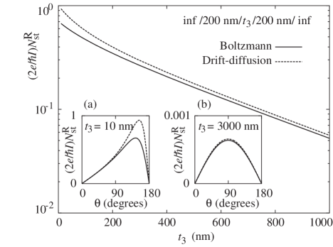
Figure 4: Spin-transfer torque at the right interface of the spacer layer in a spin valve with semi-infinite leads. Solid curves are calculated from the Boltzmann equation, dashed curves are from the drift-diffusion method. The two insets show the angular dependence of the torque for two specific thicknesses, $t_{3}=$ 10 nm (a) and 3000 nm (b). The main panel shows the thickness dependence of the maximum values as a function of angle for the two approaches. The legend gives the thicknesses of the layers (inf=infinite).

The torques decrease with thickness for two reasons. The large length scale decay is set by the spin diffusion length. When the layer is thicker than its spin diffusion length, spin-flip scattering leads to a significant decrease in the polarization of the current that crosses from one side to the other. For spacer layers thinner than their spin diffusion length, but longer than their mean free paths, the polarization of the current depends on the ratio of the effective polarized resistance to the effective unpolarized resistance. For these structures, in which the ferromagnetic layers are thicker than their spin diffusion length, the polarization of the current decays roughly like one over the thickness of the spacer layer.

The final situation, in which the drift-diffusion approach is not adequate to describe the full angular dependence of the distribution function, is at the interfaces between the leads and the reservoirs. Typically, in the drift-diffusion approach, the spin accumulation is set to zero at this point and the spin current is allowed to vary. The argument is roughly that the large total density of states there compared to in the leads forces the spin accumulation to be small. In Sec. 3.6.2, we described how the greater flexibility available in the Boltzmann equation allows the implementation of boundary conditions that treat the reservoir as an absorber. In Figure 5, we show the differences that can result from the differences in the boundary conditions. Both calculations show that the angular variation in the torque depends strongly on the length of the leads. However, the Boltzmann equation results are not as sensitive as those from the drift diffusion calculation. In fact, the drift diffusion calculation gives both the parallel and antiparallel states as unstable for an asymmetric enough junction.

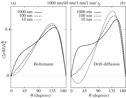
Figure 5: Spin-transfer torque at the right interface of the spacer layer in a spin valve. The left panel is calculated using the Boltzmann equation, the right panel using the drift-diffusion method. The legend gives the thicknesses of the layers.

The results described above show that the drift diffusion approach does not work when the layers are thin. Slonczewski Xiao:2004 ; Slonczewski:2002 , developed a simple hybrid theory that overcomes some of these difficulties. In particular, it treats the left going and right going electrons in the spacer layer separately. This overcomes the errors illustrated in Figure 4. The theory then treats the transport in the rest of the system with an approach closely related to circuit theory Brataas:2000 ; Brataas:2001 . The result is an analytic expression for the torque, Eq. (111). Here, we compare this hybrid theory with the Boltzmann equation to test its validity. In addition, we explore the systematic behavior of the spin-transfer torque as a function of the spin valve geometry. Figure 6 shows the angular dependence of the spin-transfer torque acting on the right FM (Co) layer for a spin valve with geometry:

$$\rm Cu(5~{}nm)/Co(40~{}nm)/Cu(t_{3})/Co(1~{}nm)/Cu(180~{}nm).$$

The spacer layer thickness $t_{3}$ varies from 1 nm to 160 nm. The magnitude of the spin-transfer torque reduces as spacer layer thickness $t_{3}$ increases. Features of the torque are discussed in Ref. Xiao:2004 .

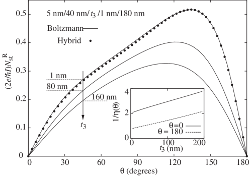
Figure 6: Spin-transfer torque at the right interface of the spacer layer in a spin valve with layer thicknesses 5 nm/40 nm/$t_{3}$/1 nm/180 nm with $t_{3}=1$ nm, 80 nm, and 160 nm. The solid curves are calculated from the Boltzmann equation. Solid circles are calculated by from the hybrid theory. The latter do not depend on $t_{3}$. The inset shows the $t_{3}$ dependence of $1/\eta(\theta)$ for $\theta=0^{\circ}$ and $180^{\circ}$ for this geometry. The legend gives the thicknesses of the layers.

In Slonczewski’s hybrid theory Xiao:2004 ; Slonczewski:2002 , scattering in the spacer layer is ignored. This means the spacer layer is treated as a thin film. In the case $t_{3}=1$ nm, the spacer layer thickness satisfies the condition of the hybrid theory. If we fit the spin-transfer torque curve calculated from the Boltzmann equation using the spin-transfer torque formula Eq. (110) from the hybrid theory (see Figure 6 for the fit), we find that the fitted interface resistance values agree with the experimental values within 15 %. This is very good agreement considering the experimental values themselves are accurate only within 10 % to 20 %. However, if the spacer layer thickness becomes comparable to the mean free path in Cu, the torque curves (the solid curve in Figure 6 with $t_{3}=80$ nm and 160 nm) cannot be fit by the hybrid theory for any values of the interface resistances.

The inset figure in Figure 6 shows how $1/\eta(0^{\circ})$ (solid line) and $1/\eta(180^{\circ})$ (dash line) vary with $t_{3}$ in the Boltzmann calculation. These quantities are related to the critical current for initiating a magnetization switching: from parallel (P) to antiparallel (AP) $J_{\rm P\rightarrow AP}\propto 1/\eta(0^{\circ})$ and from antiparallel to parallel $J_{\rm AP\rightarrow P}\propto 1/\eta(180^{\circ})$. So the curves in the inset figure of Figure 6 also show that the critical currents vary almost linearly with the spacer layer thickness $t_{3}$, and both curves have similar slopes. Experimental measurements show the critical currents increasing with spacer layer thickness Albert:2002 .

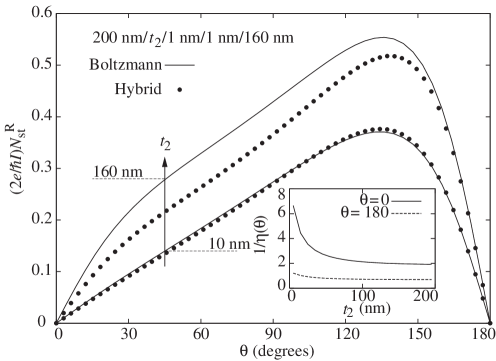
Figure 7: Spin-transfer torque at the right interface of the spacer layer in a spin valve with layer thicknesses 200 nm/$t_{2}$/1 nm/1 nm/160 nm with $t_{2}=10$ nm and 160 nm. Solid curves are calculated from the Boltzmann equation, solid circles are from the hybrid theory. The inset shows the $t_{2}$ dependence of $1/\eta(\theta)$ for $\theta=0^{\circ}$ and $180^{\circ}$. The legend gives the thicknesses of the layers.

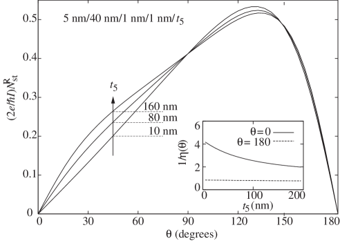
Figure 8: Spin-transfer torque at the right interface of the spacer layer in a spin valve with layer thicknesses 5 nm/40 nm/1 nm/1 nm/$t_{5}$ with $t_{5}=10$ nm, 80 nm, and 160 nm. All solid curves are calculated from the Boltzmann equation. The inset shows the $t_{5}$ dependence of $1/\eta(\theta)$ for $\theta=0^{\circ}$ and $180^{\circ}$ for this geometry. The legend gives the thicknesses of the layers.

We have seen in Figure 6 that Slonczewski’s hybrid theory fails when the spacer layer is thick. The breakdown of the hybrid theory is also seen in Figure 7, where we show how the spin-transfer torque curve changes with the thickness of the left ferromagnetic layer $t_{2}$. The input values in the hybrid theory here in Figure 7 are the same as those used in Figure 6. In the case $t_{2}=10$ nm, which is small compared to the spin flip length $l_{\rm sf}^{F}=59$ nm in the ferromagnet, the hybrid theory and the Boltzmann calculation agree with each other very well. When $t_{2}=160$ nm, $t_{2}$ becomes comparable to or larger than $l_{\rm sf}^{F}$, the hybrid theory starts to fail because an approximation of the hybrid theory does not hold when $t_{2}\gtrsim l_{\rm sf}^{F}$. This approximation assumes the spin currents at two sides of the thick ferromagnetic layer are equal: $Q(x_{1})\simeq Q(x_{2})$ (see Figure 2). But in this case of $t_{2}\gtrsim l_{\rm sf}^{F}$, $Q(x_{1})$ depends on $t_{2}$ in a non-trivial way.

Next, we study a spin valve with geometry:

$$\rm Cu(5~{}nm)/Co(40~{}nm)/Cu(1~{}nm)/Co(1~{}nm)/Cu(t_{5}),$$

where the right lead length $t_{5}$ varies from 10 nm to 160 nm. Figure 8 shows how the spin-transfer torque curve acting on the second (thin) Co layer changes when we vary $t_{5}$. A second bump around $\theta=30^{\circ}$ appears in Figure 8 as $t_{5}$ becomes large. From the spin-transfer torque formula Eq. (110) and Eq. (111) in the hybrid theory, we see that the second bump corresponds to the $q_{-}$ term in Eq. (111). The value of $q_{-}$ is typically close to zero and negligible, but it becomes prominent when the spin valve is highly asymmetric. By asymmetry, we mean that the left and right sides of the spacer layer have different spin dependent properties. For instance, for a spin valve with the geometry

$$\rm Cu(5~{}nm)/Co(40~{}nm)/Cu(1~{}nm)/Co(1~{}nm)/Cu(160~{}nm),$$

the left side of the spacer layer has 5 nm Cu, and 40 nm Co, and two Cu/Co interfaces, which can be considered mostly ferromagnetic, because both Co and Cu/Co interfaces have spin dependent resistances. However, on the right side of the spacer layer, there is only 1 nm of Co, while there are 160 nm Cu and two Cu/Co interfaces. So the 160 nm Cu dilutes the ferromagnetic character of the Co bulk and the Cu/Co interfaces and makes the right side of the spacer layer more like a non-magnet. This asymmetry of the spin valve – ferromagnet-like on the left and non-magnet-like on the right – leads to the emergence of the second bump in Figure 8.

5 Summary

In summary, we developed a complete numerical algorithm to solve the Boltzmann equation in multilayer heterostructures using a scattering matrix formalism. This method solves the spin-dependent Boltzmann equation in a non-magnet and a ferromagnet and matches the bulk solutions using an interface scattering matrix for the distribution functions. The final solution for the distribution function is found by imposing boundary conditions, either from infinite leads or from the electron reservoirs. Our interest in using this method is to calculate spin-transfer torque in a spin valve structure. The results were found to agree with the Slonczewski’s hybrid theory for geometries typically encountered in experiments but not when layer thicknesses become large compared to mean free paths. The drift-diffusion method agrees poorly with the Boltzmann calculation due to the extreme approximations it makes.

One of us (J.X.) is grateful for support from the Department of Energy under Grant No. DE-FG02-04ER46170.

References

- (1) J.C. Slonczewski, J. Magn. Magn. Mater. 159, L1 (1996)
- (2) L. Berger, Phys. Rev. B 54, 9353 (1996)
- (3) J.A. Katine, F.J. Albert, R.A. Buhrman, E.B. Myers, D.C. Ralph, Phys. Rev. Lett. 84, 3149 (2000)
- (4) S. Urazhdin, N.O. Birge, W.P. Pratt, Jr., J. Bass, Phys. Rev. Lett. 91, 146803 (2003)
- (5) S.I. Kiselev, J.C. Sankey, I.N. Krivorotov, N.C. Emley, R.J. Schoelkopf, R.A. Buhrman, D.C. Ralph, Nature 425, 380 (2003)
- (6) W.H. Rippard, M.R. Pufall, S. Kaka, S.E. Russek, T.J. Silva, Phys. Rev. Lett. 92, 27201 (2004)
- (7) A. Fert, V. Cros, J. M. George, J. Grollier, H. Jaffrès, A. Hamzić, A. Vaurès, G. Faini, J. Ben Youssef, and, H. Le Gall J. Magn. Magn. Mater. 272-76, 1706 (2004)
- (8) J.Z. Sun, Phys. Rev. B 62, 570 (2000)
- (9) D.H. Hernando, Y.V. Nazarov, A. Brataas, G.E.W. Bauer, Phys. Rev. B 62, 5700 (2000)
- (10) X. Waintal, E.B. Myers, P.W. Brouwer, D.C. Ralph, Phys. Rev. B 62, 12317 (2000)
- (11) M.D. Stiles, A. Zangwill, Phys. Rev. B 66, 14407 (2002)
- (12) Z. Li, S. Zhang, Phys. Rev. B 68, 24404 (2003)
- (13) Y.B. Bazaliy, B.A. Jones, S.C. Zhang, Phys. Rev. B 69, 94421 (2004)
- (14) M.D. Stiles, A. Zangwill, J. Appl. Phys. 91, 6812 (2002)
- (15) J. Xiao, A. Zangwill, M.D. Stiles, Phys. Rev. B 70, 172405 (2004)
- (16) D.M. Edwards, F. Federici, J. Mathon, A. Umerski, Phys. Rev. B 71, 054407 (2005)
- (17) L. Berger, IEEE Trans. Magn. 34, 3837 (1998)
- (18) J. Grollier, V. Cros, H. Jaffrès, A. Hamzić, J. M. George, G. Faini, J. Ben Youssef, H. Le Gall, and A. Fert, Phys. Rev. B 67, 174402 (2003)
- (19) M.D. Stiles, J. Xiao, A. Zangwill, Phys. Rev. B 69, 54408 (2004)
- (20) J. Barnas, A. Fert, M. Gmitra, I. Weymann, and V. K. Dugaev, Phys. Rev. B 72, 024426 (2005)
- (21) A. Brataas, Y.V. Nazarov, G.E.W. Bauer, Phys. Rev. Lett. 84, 2481 (2000)
- (22) A. Brataas, Y.V. Nazarov, G.E.W. Bauer, Euro. Phys. J. B 22, 99 (2001)
- (23) P. Zahn, I. Mertig, M. Richter, and H. Eschrig, Phys. Rev. Lett. 75, 2996 (1995)
- (24) P. Zahn, J. Binder, and I. Mertig, Phys. Rev. B 72, 174425 (2005)
- (25) J.C. Slonczewski, J. Magn. Magn. Mater. 247, 324 (2002)
- (26) D.R. Penn, M.D. Stiles, Phys. Rev. B 59, 13338 (1999)
- (27) W.H. Press, B.P. Flannery, S.A. Teukolsky, W.T. Vetterling, Numerical Recipes (Cambridge University Press, 1986)
- (28) V. K. Dugaev, V. I. Litvinov, and P. P. Petrov Phys. Rev. B 52, 5306 (1995)
- (29) Shufeng Zhang and Peter M. Levy Phys. Rev. Lett. 77, 916 (1996)
- (30) K. Xia, M. Zwierzycki, M. Talanana, P. J. Kelly, and G. E. W. Bauer Phys. Rev. B 73, 064420 (2006)
- (31) L. Berger, J. Magn. Magn. Mater. 278, 185 (2004)
- (32) J. Hamrle, T. Kimura, T. Yang, Y. Otani, J. Appl. Phys. 98, 064301 (2005)
- (33) M.D. Stiles, D.R. Penn, Phys. Rev. B 61, 3200 (2000)
- (34) J. Bass, W.P. Pratt, Jr., J. Magn. Magn. Mater. 200, 274 (1999)
- (35) Q. Yang, P. Holody, S.F. Lee, L.L. Henry, R. Loloee, P.A. Schroeder, J. W. P. Pratt, J. Bass, Phys. Rev. Lett. 72, 3274 (1994)
- (36) J. Manschot, A. Brataas, G.E.W. Bauer, Phys. Rev. B 69, 92407 (2004)
- (37) M. D. Stiles, J. Appl. Phys. 79, 5805 (1996)
- (38) F.J. Albert, N.C. Emley, E.B. Myers, D.C. Ralph, R.A. Buhrman, Phys. Rev. Lett. 89, 226802 (2002)