Density of near-extreme events

Abstract

We provide a quantitative analysis of the phenomenon of crowding of near-extreme events by computing exactly the density of states (DOS) near the maximum of a set of independent and identically distributed random variables. We show that the mean DOS converges to three different limiting forms depending on whether the tail of the distribution of the random variables decays slower than, faster than, or as a pure exponential function. We argue that some of these results would remain valid even for certain correlated cases and verify it for power-law correlated stationary Gaussian sequences. Satisfactory agreement is found between the near-maximum crowding in the summer temperature reconstruction data of western Siberia and the theoretical prediction.

Extreme value statistics (EVS) EVT , —the statistics of the maximum or the minimum value of a set of random observations,— has seen a recent resurgence of interests due to its applications found in diverse fields such as physics physics , engineering engineering , computer science KM , finance finance , hydrology hydrology , and atmospheric sciences climate . In particular, for independent and identically distributed (i.i.d.) observations from a common probability density function (PDF) $p(X)$, the EVS is governed by one of the three well known limit laws EVT , namely, (a) Fréchet, (b) Gumbel, or (c) Weibull, depending on whether the tail of $p(X)$ is, (a) power-law, (b) faster than any power-law but unbounded, or (c) bounded, respectively. Recently, these same limiting laws have also been observed in a seemingly different problem concerning the level density of a Bose gas and integer partition problem comtet .

While EVS is very important, an equally important issue concerns the near-extreme events near-maxima , —i.e., how many events occur with their values near the extreme? In other words, whether the global maximum (or minimum) value is very far from others (is it lonely at the top?), or there are many other events whose values are close to the maximum value. This issue of the crowding of near-extreme events arises in many problems. For instance, in disordered systems, the low temperature properties are governed by the spectral density function of the excited states near the ground state. In the study of weather and climate extremes, an important question is: how often do extreme temperature events such as heat waves and cold waves occur? While for an insurance company, it is very important to safeguard itself against excessively large claims, it is equally or may be more important to guard itself from unexpectedly high number of them. In many of the optimization problems finding the exact optimal solution is extremely hard and only practical solutions available are the near-optimal ones optimization . In these situations, the prior knowledge about the crowding of the solutions near the optimal one is very much desirable.

In this Letter, we study quantitatively the phenomenon of the crowding of events near the extreme value for i.i.d. random variables, and find rather rich and often universal behavior. In general, the events that occur in nature are correlated. However, when the correlations among them are not very strong, then their EVS converges to that of the i.i.d. random variables berman . This is why the limiting laws of EVS of the i.i.d. random variables are very useful. Here we consider i.i.d. random variables in the similar spirit of the random-energy model derrida for disordered systems, —which despite its simplicity that the energy levels are i.i.d. random variables, has been successful in capturing many qualitative features of complex spin-glass systems. Moreover, we provide an example of a power-law correlated case, where the behavior of near-extreme events converges to that of the i.i.d. random variables. In addition, by comparing the near-maximum crowding in the reconstructed summer temperature data of western Siberia against the prediction from the i.i.d. random variables, we find satisfactory agreement.

We start with a sequence of $N$ i.i.d. random observations $\{X_{1},X_{2},\ldots X_{N}\}$, drawn from a common PDF $p(X)$. Let $X_{\max}$ be the maximum of the sequence, —i.e., $X_{\max}=\max(X_{1},X_{2},\ldots X_{N})$. A natural measure of the crowding of events near $X_{\max}$, is the density of states (DOS) with respect to the maximum

$$\rho(r,N)=\frac{1}{N}\sum_{\{X_{i}\neq X_{\max}\}}^{N-1}\delta\left[r-(X_{\max}-X_{i})\right],$$ (1)

where $r$ is measured from the maximum value, and we do not count $X_{\max}$ itself, —i.e., $\int_{0}^{\infty}\rho(r,N)\,dr=1-1/N$. Clearly, $\rho(r,N)$ fluctuates from one realization of the random sequence to another, and one is interested in knowing whether its statistical properties show any general limiting behavior, in the same sense, as one finds for the EVS. Note that, even though the random variables are independent, the different terms in Eq. (1) become correlated through their common maximum $X_{\max}$.

We find that the mean DOS $\overline{\rho(r,N)}$ displays rather rich limiting behavior, as $N\rightarrow\infty$. If the tail of the parent distribution $p(X)$ of the random variables decays slower than a pure exponential function, the behavior of $\overline{\rho(r,N)}$ is governed by the corresponding extreme value distribution. On the other hand, when the tail of $p(X)$ is faster than a pure exponential, it is related to the parent distribution itself. In the borderline case when $p(X)$ has a pure exponential tail, $\overline{\rho(r,N)}$ is entirely different.

To find $\overline{\rho(r,N)}$, first consider Eq. (1) for a given value of the maximum at $X_{\max}=x$. Then the rest of the $(N-1)$ variables are distributed independently according to the common conditional PDF $p_{\text{cond}}(X,x)=p(X)/\int_{-\infty}^{x}p(y)\,dy$. Hence the conditional mean DOS, from Eq. (1), is $\overline{\rho_{\text{cond}}(r,N,x)}=[(N-1)/N]\,p_{\text{cond}}(x-r,x)$. For a set of $N$ i.i.d. random variables, the PDF of their maximum value $X_{\max}=x$ is

$$p_{\max}(x,N)=Np(x)\left[\int_{-\infty}^{x}p(y)\,dy\right]^{N-1}.$$ (2)

Thus, $\overline{\rho(r,N)}=\int_{-\infty}^{\infty}\overline{\rho_{\text{cond}}(r,N,x)}\,p_{\max}(x,N)\,dx$. Upon substituting the expressions for $\overline{\rho_{\text{cond}}(r,N,x)}$ and $p_{\max}(x,N)$, a little algebra shows that

$$\overline{\rho(r,N)}=\int_{-\infty}^{\infty}p(x-r)\,p_{\max}(x,N-1)\,dx.$$ (3)

This is the key result, which is valid for all $N$. We next analyze its limiting behavior for large $N$.

For i.i.d. random variables, it is known that $p_{\max}(x)$ has a limiting distribution EVT :

$$b_{N}\,p_{\max}(x=a_{N}+b_{N}z,N)\xrightarrow{N\rightarrow\infty}f(z).$$ (4)

The non-universal scale factors $a_{N}$ and $b_{N}$ depend explicitly on the parent distribution $p(X)$ and $N$. However, the scaling function $f(z)$ is universal and belongs to (a) Fréchet, (b) Gumbel, or (c) Weibull, depending only on the tail of $p(X)$. For example, if $p(X)\sim\exp(-X^{\delta})$ for large $X$, then $a_{N}\sim(\ln N)^{1/\delta}$ and $b_{N}\sim\delta^{-1}(\ln N)^{1/\delta-1}$ for large $N$, and the scaling function is the universal Gumbel PDF $f(z)=\exp\left[-z-\exp(-z)\right]$. Note that, as $N\rightarrow\infty$, for $\delta<1$, $b_{N}\rightarrow\infty$, whereas $b_{N}\rightarrow 0$ for $\delta>1$. In fact, this large $N$ behavior of $b_{N}$ is not restricted to only this specific tail of $p(X)$, but is more generic: for any slower than $\exp(-X)$ tail of $p(X)$, as $N$ increases $b_{N}$ also increases, whereas for any faster than $\exp(-X)$ tail, $b_{N}$ decreases as $N$ increases. This is indeed responsible for the generic limiting behavior of $\overline{\rho(r,N)}$.

When $p(X)$ has a slower than exponential tail, so that $b_{N}\rightarrow\infty$ as $N\rightarrow\infty$, it is useful to make a change of variable $x=a_{N}+b_{N}z$ in Eq. (3). Then one immediately realizes that $p(b_{N}z+a_{N}-r)$ is highly localized, in the limit $N\rightarrow\infty$, compared to $f(z)$, —i.e., $b_{N}p(b_{N}z+a_{N}-r)\rightarrow\delta(z-[r-a_{N}]/b_{N})$. Therefore, in the scaling region of order $b_{N}$, around $r=a_{N}$

$$\overline{\rho(r,N)}\xrightarrow{N\rightarrow\infty}\frac{1}{b_{N}}f\left(\frac{r-a_{N}}{b_{N}}\right).$$ (5)

On the other hand, if the tail of $p(X)$ is faster than exponential, so that $b_{N}\rightarrow 0$ as $N\rightarrow\infty$, the PDF of the maximum becomes highly localized near $x=a_{N}$, —i.e., $p_{\max}(x,N)\rightarrow\delta(x-a_{N})$. Therefore, Eq. (3) yields

$$\overline{\rho(r,N)}\xrightarrow{N\rightarrow\infty}p(a_{N}-r).$$ (6)

In EVS, the convergence towards the limiting distribution is usually very slow slow-convergence . Therefore, it is instructive to check how $\overline{\rho(r,N)}$ approaches the limiting form for large $N$. For this purpose, now we consider explicit forms of $p(X)$, such that $\overline{\rho(r,N)}$ can be computed to high accuracy for any given $N$ by numerically integrating Eq. (3), and also the explicit forms for $a_{N}$ and $b_{N}$ as a function of $N$ can be obtained. The mean number of events close to the maximum, for a finite but large sample of size $N$, is proportional to $\overline{\rho(0,N)}$. In certain cases, $r=0$ is part of the scaling function and $\overline{\rho(0,N)}$ can be obtained from the scaling form of $\overline{\rho(r,N)}$ by putting $r=0$. However, sometimes $r=0$ is not part of the scaling regime and $\overline{\rho(0,N)}$ has to be computed separately from Eq. (3). For simplicity, we consider only positive random variables.

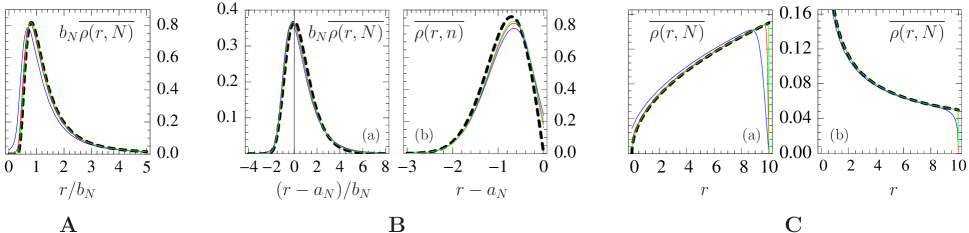
Figure 1: (Color online). A: $\overline{\rho(r,N)}$ for $N=10^{2}$ (blue), $10^{3}$ (red) and $10^{4}$ (green), for the power-low distribution $p(X)=\alpha\exp(-X^{-\alpha})X^{-(1+\alpha)}$, with $\alpha=2$. The dashed (black) line plots the Fréchet distribution $f_{1}(r/b_{N})$. B: $\overline{\rho(r,N)}$ for exponential decay $p(X)=\delta X^{\delta-1}\exp(-X^{\delta})$. (a) For $\delta=1/2$, with $N=10^{3}$ (blue), $10^{5}$ (red) and $10^{7}$ (green). The dashed (black) line plots the Gumbel distribution $f_{2}([r-a_{N}]/b_{N})$. (b) For $\delta=2$, with $N=10^{3}$ (blue), $10^{6}$ (red) and $10^{9}$ (green). The dashed (black) line plots $p(a_{N}-r)$. C: $\overline{\rho(r,N)}$ for bounded distribution, $p(X)=\beta a^{-\beta}(a-X)^{\beta-1}$ for $X<a$ and $p(X)=0$ for $X\geq a$, where $a=10$. (a) For $\beta=3/2$, with $N=10^{2}$ (blue), $10^{3}$ (red) and $10^{4}$ (green). (b) For $\beta=1/2$, with $N=10$ (blue), $10^{2}$ (red) and $10^{3}$ (green). The dashed (black) lines plot $p(a-r)$.

A. Power-law tail.— Consider $p(X)=\frac{\alpha\exp(-X^{-\alpha})}{X^{1+\alpha}}$, where $\alpha>0$. In this case, $a_{N}=0$ and $b_{N}=N^{1/\alpha}$. Therefore, limiting $\overline{\rho(r,N)}$ is given by Eq. (5), with $f(z)$ belonging to the Fréchet class:

$$f(z)\equiv f_{1}(z)=\frac{\alpha\exp\left[-z^{-\alpha}\right]}{z^{1+\alpha}},\quad z\geq 0.$$ (7)

Figure. 1A compares this limiting form with the results obtained from Eq. (3) by evaluating the integration numerically. Here, $r=0$ is away from the scaling regime. Thus, $\overline{\rho(0,N)}$ is obtained directly from Eq. (3),

$$\overline{\rho(0,N)}\xrightarrow{N\rightarrow\infty}\frac{\alpha\Gamma(2+1/\alpha)}{N^{1+1/\alpha}}.$$ (8)

B. Faster than power-law, but unbounded tail.— Consider $p(X)=\delta X^{\delta-1}\exp(-X^{\delta})$, where $\delta>0$. In this case $a_{N}=(\ln N)^{1/\delta}$ and $b_{N}=\delta^{-1}(\ln N)^{1/\delta-1}$. For very large and very small $r$, the large $N$ forms of the mean DOS have same forms for all $\delta$, —i.e., $\overline{\rho(r,N)}\sim Np(r)$ for $r\gg a_{N}$, and $\overline{\rho(r,N)}\approx p(a_{N}-r)$ for $r\ll a_{N}$. Thus, at $r=0$

$$\overline{\rho(0,N)}\xrightarrow{N\rightarrow\infty}p(a_{N})=\frac{\delta}{N}(\ln N)^{1-1/\delta},$$ (9)

for all $\delta$. However, the scaling behaviors of $\overline{\rho(r,N)}$ are very different for the three cases: $\delta<1$, $\delta=1$, and $\delta>1$.

Case I: $\delta<1$. As $N\rightarrow\infty$, $b_{N}\rightarrow\infty$. Therefore, in the scaling regime around $r=a_{N}$, —which, however, becomes larger as $N$ increases, as $b_{N}$ becomes larger— the limiting $\overline{\rho(r,N)}$ is again given by Eq. (5), but now $f(z)$ belongs to the Gumbel class:

$$f(z)\equiv f_{2}(z)=\exp\left[-z-\exp(-z)\right].$$ (10)

Figure. 1B (a) compares the limiting form with the results obtained from Eq. (3) by numerical integration.

Case II: $\delta=1$. In this case $b_{N}=1$. In this borderline case neither of the limiting forms, —i.e., Eq. (5) or (6), are reached in the large $N$ limit. Instead, we find a completely different behavior: $\overline{\rho(r,N)}=g(r-a_{N})$, where the scaling function

$$g(z)=e^{z}\left[1-\left(1+e^{-z}\right)e^{-e^{-z}}\right].$$ (11)

Case III: $\delta>1$. As $N\rightarrow\infty$, $b_{N}\rightarrow 0$. Thus, $\overline{\rho(r,N)}$ now converges to the other form given by Eq. (6), which is compared in Fig. 1B (b), with the results obtained from Eq. (3) by evaluating the integration numerically.

C. Bounded tail.— Consider $p(X)=\beta a^{-\beta}(a-X)^{\beta-1}$ for $0<X<a$, where $\beta>0$, and $p(X)=0$ otherwise. In this case, $a_{N}=a$ and $b_{N}=aN^{-1/\beta}$. Therefore, again $\overline{\rho(r,N)}$ now converges to the other form given by Eq. (6). The comparison with Eq. (3) is illustrated in Fig. 1C. Again, $N$ dependence of $\overline{\rho(0,N)}$ for large $N$, does not follow from the limiting $\overline{\rho(r,N)}$. This is obtained directly from Eq. (3),

$$\overline{\rho(0,N)}\xrightarrow{N\rightarrow\infty}\frac{(\beta/a)\Gamma(2-1/\beta)}{N^{1-1/\beta}},~{}\text{for}~{}\beta>1/2.$$ (12)

To summarize the explicit results: When the tail of $p(X)$ is either power-law or bounded, the convergence of $\overline{\rho(r,N)}$ to the respective limits given by Eqs. (5) and (6) are fast, as can be seen from Figs. 1A and 1C respectively. However, in the intermediate situation —i.e., when $p(X)$ decays faster than power-law but not bounded, — the convergence is slow, as can be seen from Figs. 1B (a) and 1B (b). In other words, the more $p(X)$ deviates from $\exp(-X)$ in either direction (slower and faster), $\overline{\rho(r,N)}$ converges more quickly (with increasing $N$) to its limiting form. As $N$ increases, the mean number of events close to the maximum, which is proportional to $\overline{\rho(0,N)}$, decreases faster for $p(X)$ with a broader tail [cf. Eqs. (8), (9) and (12)]. This is also evident from the small $r$ behavior of $\overline{\rho(r,N)}$ in the scaling regime, —i.e., from the peak to the left in Figs. 1A and 1B (a): For $p(X)$ with a power-law tail, $\overline{\rho(r,N)}$ has an essential singular behavior $\exp(-N/r^{\alpha})$ for small $r$ [cf. Eq. (7)], and for a stretched-exponential tail (B with $\delta<1$), as $r$ decreases from $a_{N}$ in the scaling regime $\overline{\rho(r,N)}$ decreases super-exponentially $\exp(-\exp([a_{N}-r]/b_{N}))$ [cf. Eq. (10)]. On the contrary, for $p(X)$ having faster than $\exp(-X)$ tail, there is crowding near the maximum value ($r=0$) [Figs. 1B (b) and 1C].

Another measure of the loneliness of the maximum is the gap between the maximum and the next highest value. Let $Q(\epsilon|N)$ be the PDF of the gap being $\epsilon$. Clearly

$$Q(\epsilon|N)=N\int_{-\infty}^{\infty}p(z+\epsilon)\,p_{\max}(z,N-1)\,dz.$$ (13)

In particular, when $p(X)\sim\exp(-X^{\delta})$ for large $X$, we find the limiting form

$$Q(\epsilon|N)\xrightarrow{N\rightarrow\infty}\frac{1}{b_{N}}\exp(-\epsilon/b_{N}).$$ (14)

Thus, the typical gap is of the order $b_{N}$, which increases (decreases) as $N$ increases for $\delta<1$ ($\delta>1$), —consistent with the results obtained form the study of mean DOS.

So far, we have considered the case of i.i.d. random variables. What would happen if the random variables are correlated? For short-ranged correlation, one expects the results from i.i.d. random variables to hold. However, for a stationary Gaussian sequence (SGS), this holds even for long-range (e.g. power-law) correlation. More precisely, for SGS a rigorous theorem berman states: if the correlator $C(n)\equiv\overline{X_{i}X_{i+n}}$ satisfies either $\lim_{n\rightarrow\infty}C(n)\ln n=0$ or $\sum_{n=1}^{\infty}C^{2}(n)<\infty$, then the limiting distribution of the maximum [cf. Eq. (4)] is Gumbel [cf. Eq. (10)], and $a_{N}$ and $b_{N}$ are same as those in the case of independent Gaussian random variables. Based on this theorem, one therefore predicts that $\overline{\rho(r,N)}$ for large $N$, should be independent of the correlation function $C(n)$ and hence would be the same as that of Gaussian i.i.d. random variables. We have indeed verified this prediction for SGS’s with a power-law correlation $C(n)=(1+n^{2})^{-\gamma/2}$, which are generated using numerical simulation. We compute $\overline{\rho(r,N)}$ from these sequences for three different values of $N$ and for each $N$ two different values of $\gamma$, and compare with the one obtained by numerically integrating Eq. (3) for same $N$ and using $p(X)=\exp(-X^{2}/2)/\sqrt{2\pi}$, —this is shown in Fig. 2. While for smaller $N$ [cf. Fig. 2 (a)] they differ, for larger $N$ [cf. Fig. 2 (c)] the difference becomes unnoticeable.

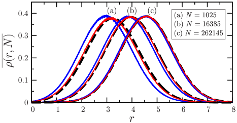
Figure 2: (Color online). $\overline{\rho(r,N)}$ for stationary Gaussian random sequence with a correlator $C(n)=(1+n^{2})^{-\gamma/2}$, where $\gamma=0.5$ (blue) and $\gamma=1$ (red) obtained from numerical simulation, and for Gaussian i.i.d. random variables (black dashed) obtained by numerical integration of Eq. (3). The three sets of curves (a), (b) and (c) correspond three different values of $N$.

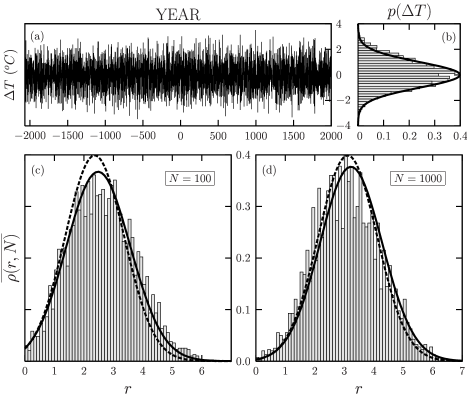
Figure 3: (a) Yamal peninsula June-July mean temperature anomaly ($\Delta T$) reconstruction series yamal_data . (b) The histogram plots the distribution $\Delta T$ of the data shown in (a). The solid line represents $p(\Delta T)=\exp(-\Delta T^{2}/2)/\sqrt{2\pi}$. In (c) and (d), the histograms plot the mean DOS relative to the maximum (excluding the maximum), computed by dividing the data into blocks, with each block consists of $N$ years. Solid lines are calculated using the exact numerical integration in Eq. (3). The dashed lines represent $p(a_{N}-r)$, where $a_{N}=(2\ln N)^{1/2}-(2\ln N)^{-1/2}(\ln\ln N+\ln 4\pi)/2$.

How well do the mathematical results describe real data? That is what we check last in this Letter, by comparing against the reconstructed Yamal multimillennial summer temperature data by Hantemirov and Shiyatov yamal_data . The reconstructed data-set consists of yearly mean summer temperature anomalies ($\Delta T)$, of Yamal Peninsula of western Siberia, relative to the mean of the full reconstructed series for 4000 years (2000 BC to AD 1996), which is shown in Fig. 3 (a). We divide the full time series into blocks of $N$ years, and for each block: (I) find the maximum value of $\Delta T$, and then (II) with respect to this maximum, compute $\rho(r,N)$ using Eq. (1). Finally, we find $\overline{\rho(r,N)}$, by taking average over all the blocks. The histograms in Fig. 3 (c) and (d) illustrate $\overline{\rho(r,N)}$, computed by dividing the full series into $40$-blocks with $100$ years of data in each block, and $4$-blocks with $1000$ years of data in each block respectively. Now to compare with our results, we first compute the distribution of $\Delta T$ from the full time series, which is illustrated in Fig. 3 (b) by histogram, along with the solid line given by the Gaussian distribution. In Fig. 3 (c) and (d), the solid lines are computed using the Gaussian distribution from Eq. (3), by performing exact numerical integration, with $N=100$ and $N=1000$ respectively. The dashed lines correspond to the limiting form $p(a_{N}-r)$, obtained in Eq. (6) for large $N$. The agreements between them (dashed and solid lines) are satisfactory.

We acknowledge the support of the Indo-French Centre for the Promotion of Advanced Research under Project 3404-2.

References

- (1) R.A. Fisher and L.H.C. Tippet, Proc. Cambridge Philos. Soc. 24, 180 (1928); E.J. Gumbel, Statistics of Extremes (Columbia University Press, NY, 1958); J. Galambos, The Asymptotic Theory of Extreme Order Statistics (John Wiley & Sons, NY, 1978).
- (2) J.-P. Bouchaud and M. Mézard, J. Phys A 30, 7997 (1997); D.S. Dean and S.N. Majumdar, Phys. Rev. E 64, 046121 (2001); G. Györgyi, P.C.W. Holdsworth, B. Portelli, and Z. Rácz, Phys. Rev. E 68, 056116 (2003); S.N. Majumdar and P.L. Krapivsky, Physica A 318, 161 (2003); J.F. Eichner, J.W. Kantelhardt, A. Bunde, and S. Havlin, Phys. Rev. E 73, 016130 (2006); E. Bertin and M. Clusel, J. Phys. A 39, 7607 (2006);
- (3) A.N. Norris, J. Mech. Materials Struct. 1, 793 (2006); A. Cazzani and M. Rovati, Int. J. Solids Struct. 42, 5057 (2005); M. Hayes and A. Shuvalov, J. appl. mech. 65, 786 (1998).
- (4) S.N. Majumdar and P.L. Krapivsky, Phys. Rev. E 65, 036127 (2002).
- (5) P. Embrechts, C. Klüppelberg, and T. Mikosch, Modelling Extremal Events for Insurance and Finance (Springer, Berlin, 1997).
- (6) R.W. Katz, M.B. Parlange, and P. Naveau, Advances in Water Resources 25, 1287 (2002).
- (7) D.R. Easterling et al., Science 289, 2068 (2000); S. Redner and M.R. Petersen, Phys. Rev. E 74, 061114 (2006).
- (8) A. Comtet, P. Leboeuf, and S.N. Majumdar, Phys. Rev. Lett. 98, 070404 (2007).
- (9) A.G. Pakes and F.W. Steutel, Aust. J. Stat. 39, 179 (1997); A.G. Pakes and Y. Li, Stat. Probab. Lett. 40, 395 (1998).
- (10) D.S. Dean, D. Lancaster, and S.N. Majumdar, Phys. Rev. E 72, 026125 (2005).
- (11) S.M. Berman, Ann. Math. Stat. 35, 502 (1964); J. Pickands, Trans. Am. Math. Soc. 145, 75 (1969).
- (12) B. Derrida, Phys. Rev. Lett. 45, 79 (1980).
- (13) G. Györgyi, N.R. Moloney, K. Ozogány, and Z. Raćz, Phys. Rev. E 75, 021123 (2007).
- (14) R.M. Hantemirov and S.G. Shiyatov, Holocene, 12, 717 (2002). Data obtained from IGBP PAGES/WDC for Paleoclimatology, http://www.ncdc.noaa.gov/paleo/pubs/hantemirov2002/