Unitary polarized Fermi gases

Abstract

Although recent theoretical and experimental progress have considerably clarified pairing mechanisms in spin 1/2 fermionic superfluid with equally populated internal states, many open questions remain when the two spin populations are mismatched. We show here that, taking advantage of the universal behavior characterizing the regime of infinite scattering length, the macroscopic properties of these systems can be simply and quantitatively understood in the regime of strong interactions.

1 Introduction

Pairing lies at the core of the standard Bardeen-Cooper-Schrieffer mechanism for metal superconductivity, and the very natural question to know whether it could survive population imbalances between the two spin states naturally arose very soon after its development [1, 2]. It was pointed out that pairing was indeed robust to some amount of mismatch between the chemical potentials of the two species, but the fate of the system after the critical imbalance is reached has long been a mystery. The absence of clear answer to this problem was due in particular to the absence of an experimental system on which the various scenarios envisioned could be tested: existence of a spatially modulated order parameter (Fulde, Ferrel, Larkin and Ovshinikov, or FFLO, phases) [3, 4, 5], or the extension to trapped systems[6, 7, 8, 9], deformed Fermi surfaces [10], interior gap superfluidity [11], phase separation between a normal and a superfluid state through a first order phase transition [12, 13, 14, 15], BCS quasi-particle interactions [16] or onset of p-wave pairing [17]. When the strength of the interactions is varied, a complicated phase diagram mixing several of these scenarios is expected [18, 19, 20].

This issue was revived by the possibility of obtaining fermionic superfluids with ultra cold atoms [21, 22, 23, 24, 25, 26], where spin imbalance could be controlled and maintained for a long time. This led to a series of experiments performed at MIT [27, 28] and Rice [29, 30] which clearly demonstrated a phase separation between regions characterized by different polarizations (i.e. spin population imbalances, by analogy with magnetism). The number of phases obtained by the two groups is however different. In Rice experiment, the cloud is constituted of a core where both spin populations are equal, surrounded by a shell of majority atoms only while at MIT a third phase mixing both species with unequal densities is intercalated between the previous ones, a discrepancy which is not yet fully explained [31, 32, 32, 33, 34, 35, 36, 37, 38].

In what follows we wish to explore the various consequences of these experiments. By contrast to most recent works on the subject, we would like to avoid the use of BCS mean field, which is known to give good qualitative insight to the problem under study, but fails when precise quantitative estimates are needed. Our scheme is based on a combination of exact variational analysis and Monte-carlo simulations. We will demonstrate that, in agreement with MIT experiments, three phases are expected in homogeneous systems. To compare with experimental results, we will make use of Local Density Approximation (LDA) which leads to quantitative agreement with MIT’s data. Finally, following [31], we will show how Rice’s apparently contradictory results can be interpreted as a breakdown of local density approximation in elongated traps.

2 Universal phase diagram of a homogeneous system

Let us first consider an ensemble of spin 1/2 fermions of mass $m$ trapped in a box of volume $V$. In the s-wave approximation, the hamiltonian $\widehat{H}$ is given by

$$\widehat{H}=\sum_{\bm{k},\sigma}\epsilon_{\bm{k}}\widehat{a}^{\dagger}_{\bm{k},\sigma}\widehat{a}_{\bm{k},\sigma}+\frac{g_{b}}{V}\sum_{\bm{k},\bm{k}^{\prime},\bm{q}}\widehat{a}^{\dagger}_{\bm{k}+\bm{q},\uparrow}a^{\dagger}_{\bm{k}^{\prime}-\bm{q},\downarrow}\widehat{a}_{\bm{k}^{\prime},\downarrow}\widehat{a}_{\bm{k},\uparrow},$$ (1)

where $\epsilon_{\bm{k}}=\hbar^{2}k^{2}/2m$, $\widehat{a}_{\bm{k},\sigma}$ annihilates a particle of spin $\sigma$ and momentum $\bm{k}$ and $g_{b}$ is the coupling constant characterizing s-wave interactions between atoms. This choice of interaction potential is singular and yields unphysical results and to get rid of the divergencies resulting by the zero range of the potential, we introduce an ultraviolet cut-off $q_{c}$ in momentum space (or equivalently, we work on a lattice of step $1/q_{c}$). When $q_{c}$ goes to infinity, the Lippmann-Schwinger formula obtained by the resolution of the two-body problem yields the following relationship between the bare coupling constant and the scattering length $a$

$$\frac{1}{g_{b}}=\frac{m}{4\pi\hbar^{2}a}-\frac{1}{V}\sum_{\bm{k}}\frac{1}{\epsilon_{\bm{k}}},$$ (2)

where the sum over $\bm{k}$ is restricted to $k<q_{c}$.

To anticipate the analysis of inhomogeneous systems, we work in the grand canonical ensemble, where the atom numbers fluctuate and only their expectation values are kept constant. Introducing the chemical potentials $\mu_{\uparrow,\downarrow}$ as Lagrange multipliers associated with the constraints on atom numbers, we need to find the ground state of the grand potential $\widehat{\Omega}$ given by

$$\widehat{\Omega}=\widehat{H}-\mu_{\uparrow}\widehat{N}_{\uparrow}-\mu_{\downarrow}\widehat{N}_{\downarrow}.$$ (3)

In what follows, we replace the minimization condition on $\Omega=\langle\widehat{\Omega}\rangle$ by a maximization problem on the pressure $P$, using the thermodynamical relation $\Omega=-PV$. Moreover, we assume $\mu_{\uparrow}>\mu_{\downarrow}$ and we restrict ourselves to the unitary limit where $a=\infty$. This choice of scattering length leads to a deep simplification of the formalism, due to the universality characterizing this regime. Indeed, from dimensional analysis [39], we can show that for an arbitrary scattering length, the pressure $P$ of a given phase is given by some relation

$$P(m,\hbar,a,\mu_{\uparrow},\mu_{\downarrow})=P_{0}(\mu_{\uparrow},\hbar,m)f(\mu_{\downarrow}/\mu_{\uparrow},1/k_{\rm F\uparrow}a),$$

where $P_{0}$ is the pressure of an ideal Fermi gas with chemical potential $\mu_{\uparrow}$ and $k_{F\uparrow}$ is the Fermi wave vector associated with $\mu_{\uparrow}$. At unitarity, $1/k_{\rm F}a=0$ and $f$ is therefore function of $\eta=\mu_{\downarrow}/\mu_{\uparrow}$ yielding the universal relation

$$\frac{P}{P_{0}}=g(\eta),$$ (4)

where $g(\mu_{\downarrow}/\mu_{\uparrow})=f(\mu_{\downarrow}/\mu_{\uparrow},0).$

Although the general minimization of the grand potential is an extremely challenging and still open problem, we first note that two exact eigenstates of the system can be found.

1. Fully polarized ideal gas. If we consider a fully polarized system containing no minority atom, the interaction term in $\widehat{H}$ disappears, and we are left with a pure ideal gas of majority atoms. The pressure of this normal phase is simply the Fermi pressure, and we have in particular $P/P_{0}=1$.

2. Fully paired superfluid. Let $|{\rm SF}\rangle_{\mu}$ be the ground state of the balanced potential $\widehat{\Omega}^{\prime}=\widehat{H}-\mu(\widehat{N}_{\uparrow}+\widehat{N}_{\downarrow})$. Since $\widehat{\Omega}^{\prime}$ commutes with the atom number operators, $|{\rm SF}\rangle_{\mu}$ can be chosen as an eigenstate of both $\widehat{N}_{\uparrow,\downarrow}$, with $\widehat{N}_{\uparrow}|{\rm SF}\rangle_{\mu}=\widehat{N}_{\downarrow}|{\rm SF}\rangle_{\mu}$. Going back to the unbalanced problem, we write $\widehat{\Omega}$ as

   $$\widehat{\Omega}=\widehat{H}+\frac{\mu_{\uparrow}+\mu_{\downarrow}}{2}(\widehat{N}_{\uparrow}+\widehat{N}_{\downarrow})+\frac{\mu_{\uparrow}-\mu_{\downarrow}}{2}(\widehat{N}_{\uparrow}-\widehat{N}_{\downarrow}).$$ (5)

   We see readily that for $\mu=(\mu_{1}+\mu_{2})/2$ we have $\widehat{\Omega}|{\rm SF}\rangle_{\mu}=\widehat{\Omega}^{\prime}|{\rm SF}\rangle_{\mu}$, which proves that $|{\rm SF}\rangle_{\mu}$ is also an eigenstate of the imbalanced grand potential. The pressure in this superfluid phase can be calculated using known results for the unitary balanced superfluid for which the universal relationship between chemical potential and density reads

   $$\mu_{\uparrow}=\mu_{\downarrow}=\xi\frac{\hbar^{2}}{2m}(6\pi^{2}n_{\uparrow})^{2/3},$$ (6)

   where $\xi\sim 0.42$ is a universal number that was evaluated both experimentally [24, 41, 40, 42, 29] and theoretically [43, 44, 45, 14]. Integrating Gibbs-Duhem identity (see appendix), one then obtains for the imbalanced system

   $$P_{\rm SF}=\frac{1}{15\pi^{2}}\left(\frac{m}{\xi\hbar^{2}}\right)^{3/2}(\mu_{\uparrow}+\mu_{\downarrow})^{5/2},$$ (7)

   hence $P_{\rm SF}/P_{0}=(1+\eta)^{5/2}/(2\xi)^{3/2}.$

The variation of the pressure versus $\eta$ is displayed in Fig. 1. We see that for small imbalances, i.e. $\eta$ smaller than $\eta_{c}=(2\xi)^{3/5}-1\sim-0.10$, the fully paired superfluid is more stable than the fully paired normal phase, confirming the stability of pairing against a small mismatch of the Fermi surfaces. The experimental results presented in ref. [28] suggest that the two classes of states we have until now restricted ourselves are not sufficient to fully capture the physics of imbalanced systems. In particular, a mixed normal phase, containing atoms of both species in unequal proportions, must be taken into account. A sketch of $g(\eta)$ for this intermediate phase is shown in Fig 1. On this more general phase diagram, the parameters $\eta_{\alpha}$ and $\eta_{\beta}$ are of special importance, since they characterize the phase transitions between the three different phases. A glance at Fig. 1 shows that they must satisfy the inequality

$$\eta_{\alpha}<\eta_{c}<\eta_{\beta},$$

and the next section is devoted to an improvement of these bounds.

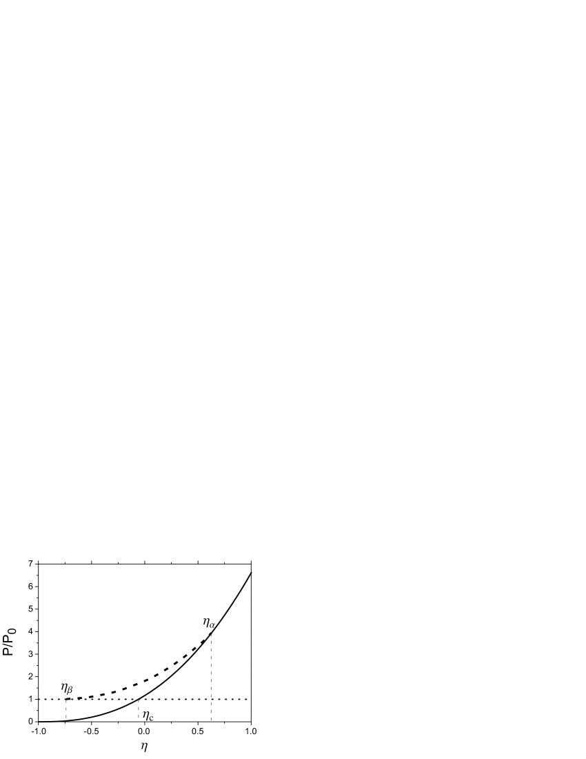
Figure 1: Sketch of the grand potential $\Omega$ as a function of $\eta=\mu_{\downarrow}/\mu_{\uparrow}$. $\Omega$ is normalized to the grand potential $\Omega_{0}$ of the pure ideal gas of chemical potential $\mu_{\uparrow}$. Full line: paired superfluid; dotted line: fully polarized normal phase; dashed line: intermediate mixed phase. $\eta_{\alpha}$ and $\eta_{\beta}$ designate the critical values for the two transitions between the superfluid/mixed phase and the mixed phase/fully polarized Fermi gas.

3 The N+1 body problem

Theoretically, the existence of the intermediate phase can be demonstrated by the study of the N+1 body problem, in other word the study of the ground state of the majority Fermi sea in the presence of a single minority atom. This particular system corresponds to an intermediate phase with $\eta\rightarrow\eta_{\beta}^{+}$ and we will prove that it yields the inequality $\eta_{\beta}<\eta_{c}$.

To address the N+1 body problem, we use a variational scheme, that we will compare to recent predictions based on Monte-Carlo simulations [46]. Let us consider the following trial state $|\psi\rangle$

$$|\psi\rangle=\phi_{0}|{\rm FS}\rangle+\sum_{\bm{k},\bm{q}}\phi_{\bm{k},\bm{q}}|\bm{k},\bm{q}\rangle,$$

where $|{\rm FS}\rangle$ is a spin up Fermi sea plus a spin down impurity with 0 momentum, and $|\bm{k},\bm{q}\rangle$ is the perturbed Fermi sea with a spin up atom with momentum $\bm{q}$ (with $q$ lower than $k_{F}$) excited to momentum $\bm{k}$ (with $k>k_{F}$). To satisfy momentum conservation, the impurity acquires a momentum $\bm{q}-\bm{k}$.

The energy of this state with respect to the non interacting ground state is $\langle\widehat{H}\rangle=\langle\widehat{H}_{0}\rangle+\langle\widehat{V}\rangle$, with

$$\langle\psi|\widehat{H}_{0}|\psi\rangle=\sum_{\bm{k},\bm{q}}|\phi_{\bm{k},\bm{q}}|^{2}(\epsilon_{\bm{k}}+\epsilon_{\bm{q}-\bm{k}}-\epsilon_{\bm{q}}),$$

and

$$\langle\psi|\widehat{V}|\psi\rangle=\frac{g_{B}}{V}\left(\sum_{\bm{q}}|\phi_{0}|^{2}+\sum_{\bm{k},\bm{k}^{\prime},\bm{q}}\phi_{\bm{k}^{\prime},\bm{q}}\phi^{*}_{\bm{k},\bm{q}}+\sum_{\bm{k},\bm{q},\bm{q}^{\prime}}\phi_{\bm{k},\bm{q}}\phi^{*}_{\bm{k},\bm{q}^{\prime}}+\sum_{\bm{q},\bm{k}}(\phi^{*}_{0}\phi_{\bm{k},\bm{q}}+\phi_{0}\phi^{*}_{\bm{k},\bm{q}})\right),$$

where $\epsilon_{\bm{k}}=\hbar^{2}k^{2}/2$, and the sums on $q$ and $k$ are implicitly limited to $q<k_{F}$ and $k>k_{F}$. As we will check later, $\phi_{\bm{k},\bm{q}}\sim 1/k^{2}$ for large momenta (see below, eqn. (10)), in order to satisfy the short range behavior $1/r$ of the pair wave function in real space. This means that most of the sums on $\bm{k}$ diverge for $k\rightarrow\infty$. This singular behavior is regularized by the renormalization of the coupling constant $g_{B}$ using the Lippman-Schwinger formula. It implies that $g_{B}$ vanishes for large cutoff, thus yielding a finite energy. However, it must be noted that the third sum in $\langle\psi|\widehat{V}|\psi\rangle$ is convergent and when multiplied by $g_{B}$ will give a zero contribution to the final energy and can therefore be omitted in the rest of the calculation.

The minimization of $\langle\widehat{H}\rangle$ with respect to $\phi_{0}$ and $\phi_{\bm{k},\bm{q}}$ is straightforward and yields the following set of equations

$$\frac{g_{B}}{V}\sum_{\bm{q}}\phi_{0}+\frac{g_{B}}{V}\sum_{\bm{q},\bm{k}}\phi_{\bm{k},\bm{q}} = E\phi_{0}{}$$ (8)

$$(\epsilon_{\bm{k}}+\epsilon_{\bm{q}-\bm{k}}-\epsilon_{\bm{q}})\phi_{\bm{k},\bm{q}}+\frac{g_{B}}{V}\sum_{\bm{k}^{\prime}}\phi_{\bm{k}^{\prime},\bm{q}}+\frac{g_{B}}{V}\phi_{0} = E\phi_{\bm{k},\bm{q}},$$ (9)

where $E$ is the Lagrange multiplier associated to the normalization of $|\psi\rangle$, and can also be identified with the trial energy. Let us introduce $\chi(\bm{q})=\phi_{0}+\sum_{\bm{k}}\phi_{\bm{k},\bm{q}}$. We see from eqn. 9 that

$$\phi_{\bm{k},\bm{q}}=-\frac{g_{B}}{V}\frac{\chi({\bm{q}})}{\epsilon_{\bm{k}}+\epsilon_{\bm{q}-\bm{k}}-\epsilon_{\bm{q}}-E}.$$ (10)

As expected, we note here the $1/\epsilon_{\bm{k}}\sim 1/k^{2}$ dependence for large $k$. Inserting this expression in the definition of $\chi$, we obtain

$$\chi(\bm{q})=\phi_{0}-\frac{g_{B}}{V}\sum_{\bm{k}}\frac{\chi(\bm{q})}{\epsilon_{\bm{k}}+\epsilon_{\bm{q}-\bm{k}}-\epsilon_{\bm{q}}-E},$$

that is

$$\chi(\bm{q})=\frac{\phi_{0}/g_{B}}{\frac{1}{g_{B}}+\frac{1}{V}\sum_{k>k_{F}}\frac{1}{\epsilon_{\bm{k}}+\epsilon_{\bm{q}-\bm{k}}-\epsilon_{\bm{q}}-E}}$$

Finally, eqn. (8) can be recast as $E\phi_{0}/g_{B}=\sum_{q<k_{F}}\chi(\bm{q})/V$, that is, using the explicit expression for $\chi(\bm{q})$:

$$E=\frac{1}{V}\sum_{q<k_{F}}\frac{1}{\frac{1}{g_{B}}+\frac{1}{V}\sum_{k>k_{F}}\frac{1}{\epsilon_{\bm{k}}+\epsilon_{\bm{q}-\bm{k}}-\epsilon_{\bm{q}}-E}}.$$

We get rid of the bare coupling constant $g_{B}$ by using the Lippman-Schwinger equation, which finally yields the following implicit equation for $E$

$$E=\frac{1}{V}\sum_{q<k_{F}}\frac{1}{\frac{m}{4\pi\hbar^{2}a}-\frac{1}{V}\sum_{k<k_{F}}\frac{1}{2\epsilon_{\bm{k}}}+\frac{1}{V}\sum_{k>k_{F}}\left(\frac{1}{\epsilon_{\bm{k}}+\epsilon_{\bm{q}-\bm{k}}-\epsilon_{\bm{q}}-E}-\frac{1}{2\epsilon_{\bm{k}}}\right)}.$$ (11)

Before addressing the unitary limit case, let us show that this formula allows us to recover the known exact results in the limit of small scattering lengths where the denominator is dominated by the $1/a$ term. The correction to the energy is therefore

$$E\sim\frac{1}{V}\sum_{q<k_{F}}\frac{4\pi\hbar^{2}a}{m}=\frac{4\pi\hbar^{2}a}{m}\frac{N}{V}$$

where $N$ is the total number of majority atoms. We thus see that the trial state recovers the mean-field prediction for low interactions. For $a\rightarrow 0^{+}$ (BEC regime), a little more involved calculation allows one to recover the classical molecular binding energy $E\sim-\hbar^{2}/ma^{2}$. Finally in the case of the unitary regime relevant to experiments, eqn. (11) is solved numerically and yields $E\sim-0.3\hbar^{2}k_{F}^{2}/m$, that is $\eta_{\beta}<-0.60$, a value remarkably close to that obtained in Monte-Carlo simulations [46].

4 Trapped system and comparison with MIT experiment

The model presented in the previous section adresses only the situation of a homogeneous system and to compare with experiments, we need to extend the formalism developed in the previous section to the case of trapped systems. To this purpose we make use of the Local Density Approximation (LDA), in which we assume that the chemical potential of species $\sigma$ varies as

$$\mu_{\sigma}(\bm{r})=\mu_{\sigma}^{0}-V(\bm{r}),$$ (12)

where $V$ is the trapping potential. From this relation, we see that varying $r$ is equivalent to varying the chemical potentials of the two species, and in particular their ratio $\eta(r)$ The two phase transitions described in the previous section will happen for radii $r=R_{\alpha,\beta}$ such that $\mu_{\downarrow}({R_{\alpha,\beta}})/\mu_{\uparrow}({R_{\alpha,\beta}})=\eta_{\alpha,\beta}$. Moreover, since the outer rim is constituted by a normal ideal gas, the boundary $R_{\uparrow}$ of the majority component is given by the condition $\mu_{\uparrow}(R_{\uparrow})=0$.

In an isotropic harmonic trap, we can combine these three relations to eliminate the parameters $\mu_{\sigma}^{(0)}$, thus obtaining the general relation relating the three radii $R_{\alpha,\beta,\uparrow}$:

$$\left(\frac{R_{\alpha}}{R_{\uparrow}}\right)^{2}=\frac{(R_{\beta}/R_{\uparrow})^{2}-q}{1-q},$$ (13)

where $q=(\eta_{\alpha}-\eta_{\beta})/(1-\eta_{\beta})$. One striking consequence of this equation is the prediction of a threshold at which $R_{\alpha}$ vanishes, corresponding to the disappearance of the fully paired superfluid. This transition happens when the ratio $(R_{\beta}/R_{\uparrow})^{2}$ reaches the critical value $q$. From the upper and lower bounds obtained for $\eta_{\alpha}$ and $\eta_{\beta}$, we see that $q>0.30$.

This prediction of LDA is remarkably well verified in MIT’s experiments [28] for which the three phases discussed above were indeed observed, and eq. (13) could be tested experimentally (Fig. 2). On this graph, we see that for large imbalance, the linear scaling predicted by eq. (13) is indeed satisfied, with $q\sim 0.32$, in agreement with the lower bound obtained earlier. The deviation from theory observed for $(R_{\beta}/R_{\uparrow})^{2}\gtrsim 0.5$ is not yet fully understood. However, it must be noted that the discrepancy takes place in a regime of low imbalance, where the phase transitions take place in the tail of the density distribution. In these regions of low density, we may observe a breakdown of the LDA, or of the hydrodynamical expansion that was used to infer the experimental radii.

The value $q\sim 0.32$ obtained from the comparison with experimental data can help us improve the bounds for $\eta_{\alpha,\beta}$. Indeed, this relation fixes the relative values of $\eta_{\alpha}$ and $\eta_{\beta}$. When combined with the bounds found in the previous section, we obtain indeed

$$-0.62 <\eta_{\beta}< -0.60$$ (14)

$$-0.10 <\eta_{\alpha}< -0.088$$ (15)

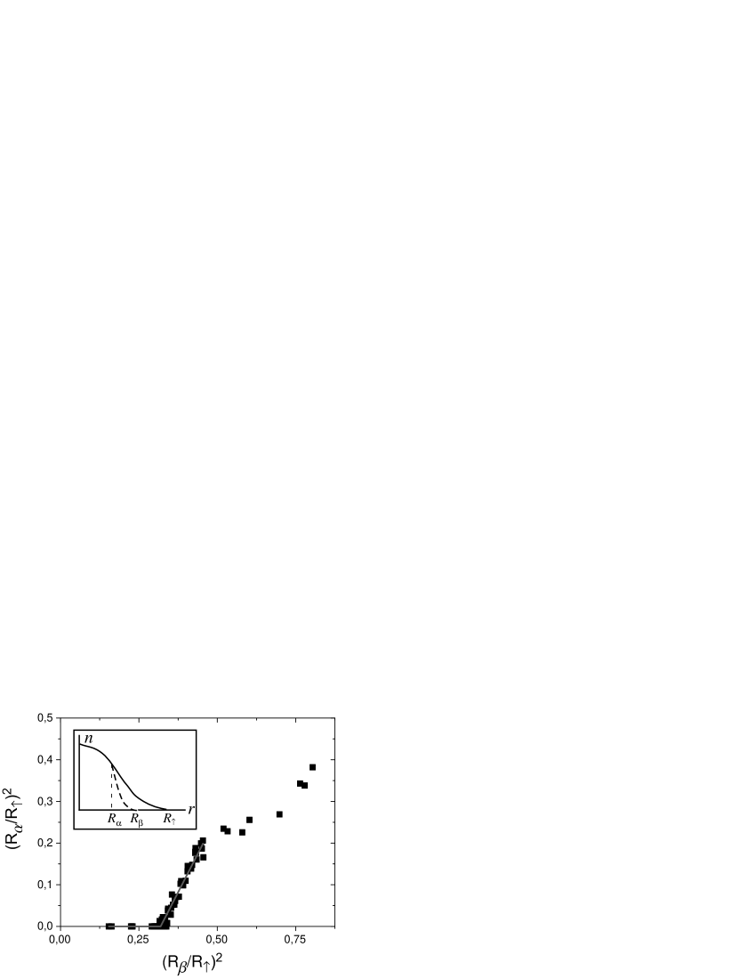
Figure 2: Comparison of equation (13) with experimental data from MIT. A fit to the data yields $q\sim 0.32$. Inset: sketch of the density profile. The full (resp. dashed) line corresponds to the density of the majority (resp. minority) component. $R_{\alpha}$ marks the end of the superfluid region, $R_{\beta}$ that of the mixture and $R_{\uparrow}$ is the frontier of the majority cloud.

From the previous analysis, we see that the combination of theoretical arguments and analysis of experimental data allows for a precise determination of the thresholds of the different phase transitions. Knowing the values of $\eta_{\alpha,\beta}$ as well as the exact equation of state in the fully polarized and fully paired phases, we can even obtain some upper and lower bounds for the equation of state of the mixed phase, using the concavity of the grand potential [36].

5 Elongated systems and Rice’s experiment

Surprisingly, similar experiments performed at Rice University showed no evidence of an intermediate phase, but rather the coexistence of the fully paired and fully polarized phases only. Measurements of the axial radii of the two phases from ref. [29] are presented in Fig. 3 and can be compared with the model presented above when omitting the intermediate mixed phase [37]. In these conditions, the inner superfluid region is now defined by the condition $\mu_{\downarrow}(\bm{r})/\mu_{\uparrow}(\bm{r})<\eta_{c}$ and is bounded by the radius $R_{\downarrow}$ defined by

$$R_{\downarrow}^{2}=\frac{2}{m\bar{\omega}^{2}}\left(\frac{\mu_{\downarrow}^{0}-\eta_{\rm c}\mu_{\uparrow}^{0}}{1-\eta_{\rm c}}\right).$$ (16)

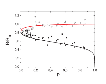
Figure 3: Rice’s radius measurement and comparison with a two phase model. The radius $R_{i}$ is scaled in units of the Thomas Fermi radius of an ideal gas with a the same atom number $N_{i}$.

Atoms of the minority species are located in the paired superfluid phase only. We thus have

$$N_{\downarrow}=\int_{r<R_{\downarrow}}n_{\downarrow}(\bm{r})\,d^{3}\bm{r}=\frac{2}{3\pi\xi^{3/2}}\left(\frac{\mu_{\uparrow}^{0}+\mu_{\downarrow}^{0}}{\hbar\bar{\omega}}\right)^{3}g(R_{\downarrow}/\bar{R}),$$ (17)

where $\bar{R}^{2}=(\mu_{\uparrow}^{0}+\mu_{\downarrow}^{0})/m\bar{\omega}^{2}$ and

$$g(x)=\frac{x\,{\sqrt{1-x^{2}}}\,\left(-3+14\,x^{2}-8\,x^{4}\right)+3\,\arcsin(x)}{48}.$$ (18)

Excess atoms of the majority species are located between $r=R_{\downarrow}$ and $r=R_{\uparrow}$ such that $m\bar{\omega}^{2}R_{\uparrow}^{2}/2=\mu_{\uparrow}^{0}$. The number of excess atoms is therefore $N_{\uparrow}-N_{\downarrow}=\int_{R_{\downarrow}}^{R_{\uparrow}}n_{1}(\bm{r})\,d^{3}\bm{r}$, hence

$$N_{\uparrow}-N_{\downarrow}=\frac{2}{3\pi}\left(\frac{2\mu_{\uparrow}^{0}}{\hbar\bar{\omega}}\right)^{3}(g(1)-g(R_{\downarrow}/R_{\uparrow})).$$ (19)

Dividing by (19) by (17) yields the implicit equation for $\eta_{0}=\mu^{0}_{\downarrow}/\mu_{\uparrow}^{0}$ as a function of $N_{\uparrow}/N_{\downarrow}$

$$\frac{N_{\uparrow}}{N_{\downarrow}}=1+\xi^{3/2}\frac{8}{(1+\eta_{0})^{3}}\frac{g(1)-g(R_{\downarrow}/R_{\uparrow})}{g(R_{\downarrow}/\bar{R})}.$$ (20)

Equation (20) is solved numerically and the value obtained for $\eta_{0}$ is then used to calculate the radii $R_{\uparrow}$ and $R_{\downarrow}$. The predicted evolution of the $R_{i}$ versus the population imbalance $P=(N_{\uparrow}-N_{\downarrow})/(N_{\uparrow}+N_{\downarrow})$ is shown in Fig. 2. To follow Ref. [29], we have normalized each $R_{i}$ to the Thomas-Fermi radius $R_{\rm TF}$ associated to an ideal gas containing $N_{i}$ atoms. The agreement with the experimental data is quite good as soon as $P\gtrsim 0.1$, a remarkable result, since the model presented here contains no adjustable parameter, as soon as the value of $\xi$ is known.

Despite this remarkable agreement, this simple two phase+local density approximation model fails to captures all experimental features. In particular, a qualitative discrepancy occurs in the comparison between the theoretical and integrated density profiles. Indeed, as shown in [47], LDA at unitarity implies a constant density difference in the paired superfluid region, in contradiction with experimental data. One solution to this problem was presented in [32, 31]. In these papers, it is noted that in the presence of phase transitions, the description of the sharp frontier separating to adjacent phases involves the introduction of density gradient terms in the energy. When the interface in thin enough, they can be encapsulated in a new surface tension energy term reading [31]

$$\Omega_{\rm ST}=\int_{\cal S}\gamma(\mu_{\uparrow\downarrow}(\bm{r}))d^{2}S,$$

where $\cal S$ is the interface between the two phases, and $\gamma$ is the surface tension constant, which should dimensionally vary as

$$\gamma=\lambda\frac{m\mu^{2}_{\uparrow}}{\hbar^{2}}.$$

Here, $\lambda$ is a numerical factor that will be determined by comparison with experiments and we have used the fact that at the coincidence between the phases, the ratio $\mu_{\downarrow}/\mu_{\uparrow}$ is fixed and equal to $\eta_{c}$, meaning that the two chemical potentials are no longer independent. We can minimize the total grand potential $\Omega=\Omega_{\rm bulk}+\Omega_{\rm ST}$, where $\Omega_{\rm bulk}=-\int\left(P_{\rm N}+P_{\rm SF}\right)d^{3}r$ is the bulk contribution to the energy. Following [31] we simplify the analysis by assuming that the interfaces are ellipsoidal, and for $\lambda\sim 10^{-4}$ one obtains the results presented in Fig. 4, which coincides with experimental data. The absence of capillary effects at MIT can be explained by a smaller trap aspect ratio and a larger atom number of atoms compared with Rice’s experimental situation, as shown by a simple scaling argument [31].

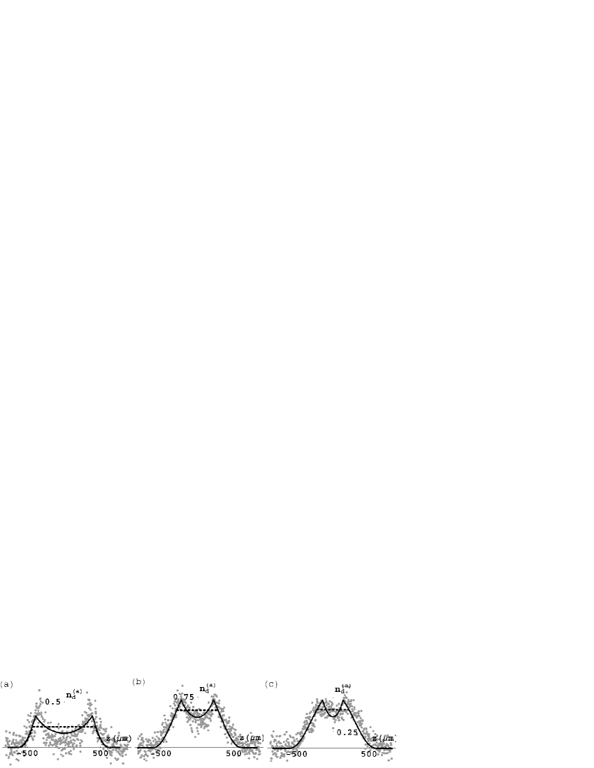
Figure 4: Integrated density difference in Rice experiments, and comparison with the surface tension model (data from [31]). Dashed line, LDA prediction: the density difference is flat in the superfluid region, in contradiction with experimental date. Full line: Two phase model incorporating surface tension effect. The same surface tension parameter $\lambda=\sim 10^{-4}$ is used for all three graphs.

6 Conclusion

The formalism presented here allows for a simple and quantitative description of macroscopic properties of polarized Fermi gases in the regime of strong interaction. This analysis is nevertheless far from being complete, since it does not give any information on the superfluid nature of the various phases. For instance, the mixed region of the phase diagram may contain superfluid and normal subdomains, the transition between this two regimes being characterized by a universal number $\eta_{\gamma}\in[\eta_{\beta},\eta_{\alpha}]$. The quantitative understanding of these superfluid properties will require beyond mean-field theories, such as the Monte-Carlo calculations of [46].

7 Acknowledgments

The author gratefully acknowledges support by the IFRAF institute and the ACI Nanosciences 2004 NR 2019. The author thanks the ENS ultracold atoms group, S. Stringari, C. Lobo, A. Recati, A. Bulgac, E.A. Mueller, X. Leyronas, C. Mora and R. Combescot for stimulating discussions. Laboratoire Kastler Brossel is a research unit No. 8552 of CNRS, ENS, and Université Paris 6.

8 Appendix: thermodynamical relations for the grand potential

Let us consider a homogeneous many-body system characterized by a hamiltonian $\widehat{H}_{0}$ and containing particles of $p$ different species labelled by $i=1..p$. In the grand canonical ensemble, one looks for the ground state of this system by letting the atom numbers fluctuate, but keeping the expectation values $\langle\widehat{N}_{i=1..p}\rangle$ fixed. This therefore requires to find the ground state of the grand potential $\widehat{\Omega}(\mu_{i})=\widehat{H}-\sum_{i=1}^{p}\mu_{i}\widehat{N}_{i}$, where the $\mu_{i}$ are Lagrange multiplier that we interpret as chemical potentials.

Let $|\psi(\mu_{i},V)\rangle$ be the ground state of the grand potential, we set $\Omega(\mu_{i},V)=\langle\psi(\mu_{i},V)|\widehat{\Omega}|\psi(\mu_{i},V)\rangle$. Using Hellman-Feynman relation, we can write that

$$\frac{\partial\Omega}{\partial\mu_{i}}=\langle\psi(\mu_{i},V)|\frac{\partial\widehat{\Omega}}{\partial\mu_{i}}|\psi(\mu_{i},V)\rangle=-\langle\widehat{N}_{i}\rangle,$$ (21)

from which we deduce that

$$d\Omega=\sum_{i}-N_{i}d\mu_{i}+\frac{\partial\Omega}{\partial V}dV.$$ (22)

By definition, and by analogie with classical thermodynamics, we identify $\partial_{V}\Omega$ with $-P$, the pressure in the system.

Let us now us the extensivity of the potential: when the volume is multiplied by some scaling factor $\lambda$, $\Omega$ is multiplied by the same factor. In other words, we have $\Omega(\lambda V,\mu_{i})=\lambda\Omega(V,\mu_{i})$. Taking $\lambda=1/V$, we get $\Omega(V,\mu_{i})=V\Omega(1,\mu_{i})$. Differentiating this with respect to $V$, we note that $\Omega(1,\mu_{i})=-P$, hence

$$\Omega=-PV$$ (23)

From this equation, we see that the minimum grand potential is state has also the highest pressure. $P$ can moreover be calculated by differentiating $\Omega$ and using equations (23) and (22). We then obtain the Gibbs-Duhem relation

$$dP=\sum_{i}n_{i}d\mu_{i},$$ (24)

where $n_{i}=N_{i}/V$ is the density of species $i$. From equation (24), we see that the pressure (hence the grand potential) can be obtained simply from the knowledge of the equation of state $n_{i}(\mu_{j})$.

8.1 Concavity

Since, by definition, $|\psi(\mu_{i})\rangle$ is the ground state of $\widehat{\Omega}(\mu_{i})$, we have for any $\delta\mu_{i}$

$$\langle\psi(\mu_{i}+\delta\mu_{i})|\widehat{\Omega}(\mu_{i})|\psi(\mu_{i}+\delta\mu_{i})\rangle\geq\langle\psi(\mu_{i})|\widehat{\Omega}(\mu_{i})|\psi(\mu_{i})\rangle$$ (25)

Moreover, if one notes that $\widehat{\Omega}(\mu_{i})=\widehat{\Omega}(\mu_{i}+\delta\mu_{i})+\sum_{j}\delta\mu_{j}\widehat{N}_{j}$, we see that for any $\delta\mu_{i}$

$$\Omega(\mu_{i}+\delta\mu_{i})+\sum_{j}\delta\mu_{j}N_{j}(\mu_{i}+\delta\mu_{i})\geq\Omega(\mu_{i})$$ (26)

Finally, recalling that $N_{i}=\partial_{\mu_{i}}\Omega$ and after expansion of equation (26) to second order in $\delta\mu_{i}$, we obtain

$$\frac{\partial^{2}\Omega}{\partial\mu_{i}\partial\mu_{j}}\delta\mu_{i}\delta\mu_{j}\leq 0,$$ (27)

hence proving the concavity of the grand-potential (or conversely the convexity of the pressure).

References

- [1] \BYA. M. Clogston \INPhys. Rev. Lett.91962266.
- [2] \BYB.S. Chandrasekhar \INAppl. Phys. Lett.119627.
- [3] \BYG. Sarma \INJournal of Physics and Chemistry of Solids2419631029.
- [4] \BYP. Fulde, R. A. Ferrell \INPhys. Rev.1351964A550.
- [5] \BYJ. Larkin, Y. N. Ovchinnikov \INSov. Phys. JETP201965762.
- [6] \BYR. Combescot \INEurophys. Lett.552001150.
- [7] \BYC. Mora \atqueR. Combescot \INPhys. Rev. B.712005214504.
- [8] \BYP. Castorina, M. Grasso, M. Oertel, M. Urban, \atqueD. Zappalà \INPhys. Rev. A722005025601.
- [9] \BYT. Mizushima, K. Machida, \atqueM. Ichioka \INPhys. Rev. Lett.942005060404; \BYT. Mizushima, K. Machida, \atqueM. Ichioka \INPhys. Rev. Lett.952005117003; \BYK. Machida, T. Mizushima, \atqueM. Ichioka \INPhys. Rev. Lett.972006120407.
- [10] \BYA. Sedrakian, J. Mur-Petit, A. Polls, \atqueH. Müther \INPhys. Rev. A722005013613.
- [11] \BYW.V. Liu \atqueF. Wilczek \INPhys. Rev. Lett.902003047002.
- [12] \BYP.F. Bedaque, H. Caldas, \atqueG. Rupak \INPhys. Rev. Lett.912003247002.
- [13] \BYH. Caldas \INPhys. Rev. A692004063602.
- [14] \BYJ. Carlson \atqueS. Reddy \INPhys. Rev. Lett.952005060401.
- [15] \BYT.D. Cohen \INPhys. Rev. Lett. 952005120403.
- [16] \BYT.-L. Ho \atqueH. Zai preprint cond-mat/0602568.
- [17] \BYA. Bulgac, Michael McNeil Forbes, \atqueA. Schwenk \INPhys. Rev. Lett.972006020402.
- [18] \BYC.H. Pao, Shin-Tza Wu \atqueS.-K. Yip \INPhys. Rev. B732006132506.
- [19] \BYD.T Son \atqueM.A. Stephanov \INPhys.Rev. A742006013614.
- [20] \BYD.E. Sheehy \atqueL. Radzihovsky \INPhys. Rev. Lett.962006060401.
- [21] \BYS. Jochim, M. Bartenstein, A. Altmeyer, G. Hendl, S. Riedl, C. Chin, J. Hecker Denschlag, \atqueR. Grimm \INScience30220032101.
- [22] \BYM.W. Zwierlein, C.A. Stan, C.H. Schunck, S.M.F. Raupach, S. Gupta, Z. Hadzibabic \atqueW. Ketterle \INPhys. Rev. Lett.912003250401.
- [23] \BYM. Greiner, C. A. Regal, \atqueD. S Jin \INNature4262003537.
- [24] \BYT. Bourdel, L. Khaykovich, J Cubizolles, J. Zhang, F. Chevy, M. Teichmann, L. Tarruell, S.J.J.M.F. Kokkelmans \atqueC. Salomon \INPhys. Rev. Lett.932004050401.
- [25] \BYJ. Kinast, S. L. Hemmer, M. E. Gehm, A. Turlapov, \atqueJ. E. Thomas \INPhys. Rev. Lett.922004150402.
- [26] \BYG. B. Partridge, K. E. Strecker, R. I. Kamar, M. W. Jack \atqueR. G. Hulet \INPhys. Rev. Lett.952005020404.
- [27] \BYM.W. Zwierlein, A. Schirotzek, C.H. Schunck, \atqueW. Ketterle \INScience3112006492.
- [28] \BYM. W. Zwierlein, C. H. Schunck, A. Schirotzek, \atqueW. Ketterle \INNature442200654.
- [29] \BYG.B. Partridge, W. Li , R.I. Kamar, Y.-A. Liao, R.G. Hulet \INScience3112006503.
- [30] \BYG. B. Partridge, Wenhui Li, Y. A. Liao, R. G. Hulet, M. Haque, H. T. C. Stoof \INPhys. Rev. Lett.972006190407.
- [31] \BYT. N. De Silva \atqueE. Mueller \INPhys. Rev. Lett.972006070402.
- [32] \BYA. Imambekov, C. J. Bolech, M. Lukin, E. Demler \INPhys. Rev. A742006053626.
- [33] \BYP. Pieri, G.C. Strinati \INPhys. Rev. Lett.962006150404.
- [34] \BYW. Yi \atqueL.-M. Duan \INPhys. Rev. A732006031604.
- [35] \BYM. Haque, \atqueH.T.C. StoofPhys. Rev. A742006011602.
- [36] \BYA. Bulgac, M. McNeil Forbes preprint cond-mat/0606043.
- [37] \BYF. Chevy \INPhys. Rev. Lett.962006130401.
- [38] \BYF. Chevy preprint cond-mat/0605751.
- [39] \BYA. Vaschy \INAnn. Tél12189225
- [40] \BYK. M. O’Hara, S. L. Hemmer, M. E. Gehm, S. R. Granade, J. E. Thomas\INScience29820022179.
- [41] \BYM. Bartenstein, A. Altmeyer, S. Riedl, S. Jochim, C. Chin, J. H. Denschlag, R. Grimm \INPhys. Rev. Lett.922004120401.
- [42] \BYJ. Kinast, A. Turlapov, J. E. Thomas, Q. Chen, J. Stajic, \atqueK. Levin \INScience30720051296.
- [43] \BYJ. Carlson, S.-Y. Chang, V. R. Pandharipande, K. E. Schmidt \INPhys. Rev. Lett.912003050401.
- [44] \BYA. Perali, P. Pieri, G. C. Strinati \INPhys. Rev. Lett.932004100404.
- [45] \BYG. E. Astrakharchik, J. Boronat, J. Casulleras, S. Giorgini\INPhys. Rev. Lett.932004200404.
- [46] \BYC. Lobo, A. Recati, S. Giorgini, S. Stringari \INPhys. Rev. Lett.972006200403
- [47] \BYT. N. De Silva, E. J. Mueller \INPhys. Rev. A73 051602(R)2006.