Griffiths singularities and algebraic order in the exact solution of an Ising model on a fractal modular network

Abstract

We use an exact renormalization-group transformation to study the Ising model on a complex network composed of tightly-knit communities nested hierarchically with the fractal scaling recently discovered in a variety of real-world networks. Varying the ratio $K/J$ of of inter- to intra-community couplings, we obtain an unusual phase diagram: at high temperatures or small $K/J$ we have a disordered phase with a Griffiths singularity in the free energy, due to the presence of rare large clusters, which we analyze through the Yang-Lee zeros in the complex magnetic field plane. As the temperature is lowered, true long-range order is not seen, but there is a transition to algebraic order, where pair correlations have power-law decay with distance, reminiscent of the $XY$ model. The transition is infinite-order at small $K/J$, and becomes second-order above a threshold value $(K/J)_{m}$. The existence of such slowly decaying correlations is unexpected in a fat-tailed scale-free network, where correlations longer than nearest-neighbor are typically suppressed.

I Introduction

Many real-world networks have modular structure GirvanNewman ; Ravasz ; NewmanGirvan ; Radicchi : their nodes are organized into tightly-knit communities where the node-node connections are dense, with sparser connections in-between communities. This structure is often hierarchically nested, with groups of communities themselves organized into higher level modules. Given the relevance of modularity to features like functional units in metabolic networks Ravasz , it is not surprising that community structure has become one of the most intensely studied aspects of complex networks. Recently, Song, Havlin and Makse Song1 ; Song2 discovered that certain modular networks also possess another remarkable characteristic: fractal scaling, where the hierarchy of modules shows a self-similar nesting at all length scales. Examples of such fractal networks include the WWW, the actor collaboration network, protein interaction networks in E. coli, yeast, and humans, the metabolic pathways in a wide variety of organisms Song1 , and genetic regulatory networks in S. cerevisiae and E. coli Yook .

Despite the widespread occurrence of fractal topologies, little is yet known about the nature of cooperative behavior on these networks, or even more generally on how modular structure affects collective ordering or correlations among interacting objects. In particular the Ising model has been investigated extensively on non-fractal scale-free networks Aleksiejuk ; Bianconi ; Dorogov0 ; Leone ; Igloi ; Goltsev ; Indekeu ; Giuraniuc1 ; Giuraniuc2 , but only recently has a form of community structure been included: an Ising ferromagnet was studied on two weakly coupled Barabasi-Albert scale-free networks with a varying density of inter-network links Suchecki , finding stable parallel and antiparallel orderings of the two communities at low temperatures. It would be interesting to examine a system with a large number of interacting communities, capturing more fully the complex modular organization of real-world examples. In this paper, we introduce a hierarchical lattice BerkerOstlund ; KaufmanGriffiths1 ; KaufmanGriffiths2 network model exhibiting a nested modular structure with fractal scaling. Hierarchical lattices (part of a broader class of deterministically constructed networks Barabasi ; Comellas ; RavaszBarabasi ; Andrade ; Doye ; Zhang1 ; ZhangComellas ; ZhangRong ; Zhang2 ; Zhang3 ) have been the focus of increasing attention recently Dorogov2 ; HinczewskiBerker ; Rozenfeld ; Zhang , since they can be tailored to exhibit various features—including scale-free degree distributions, small-world behavior, and fractal structure—for which exact analytical expressions can be derived. The explicit results from such deterministic models can serve as a testing ground for approximate phenomenological approaches, and a starting point for extensions incorporating additional realistic features like randomness Zhang .

Here we exploit another advantage of such lattices: the ferromagnetic Ising model can be solved through an exact renormalization-group (RG) transformation. Varying the strength of interactions between communities, we find an unusual combination of thermodynamic properties. At high temperatures or weak inter-community coupling the system is disordered, but the free energy as a function of magnetic field $H$ is nonanalytic at $H=0$. This is due to the presence of rare large communities, similar to the Griffiths singularity in bond-diluted ferromagnets below the percolation threshold Griffiths : there the system is partitioned into disjoint clusters of connected sites, and the small probability of arbitrarily large clusters leads to an analogous nonanalyticity in the free energy above $T_{c}$. As we lower the temperature in our network, true long-range order is never achieved at $T>0$, even for the strongest inter-community coupling. Surprisingly, we find instead a low-temperature phase with algebraic order, just as in the $XY$ model: the magnetization is zero, but there is power-law decay of pair correlations with distance, and the thermodynamic functions throughout the entire phase behave as if at a critical point.

The organization of the paper is as follows: in Sec. II we describe the network’s construction (Sec. II.A) and summarize its topological properties (Sec. II.B), including its community structure and fractal scaling characteristics. Sec. III examines thermodynamic properties of the Ising model on the network, derived from an exact renormalization-group approach (Sec. III.A). We discuss the phase diagram and critical behavior in Sec. III.B, and then focus on two particularly interesting aspects of the results: the presence of Griffiths singularities in the free energy (Sec. III.C), and the nature of long-range pair correlations in the low-temperature phase (Sec. III.D). We present our conclusions in Sec. IV, and note that the behavior described here is characteristic of a broader class of hierarchical lattice complex networks—a fact that will be explored in future studies.

II Network Properties

II.1 Construction procedure

Our lattice has two types of bonds, depicted as solid and dashed lines respectively. At each construction step, every solid bond is replaced by the connected cluster on the right of Fig. 1(a), and this procedure is iterated $t$ times. The initial $t=0$ lattice is two sites connected by a single solid bond. Fig. 1(b) shows the network at $t=4$. All results quoted below are for the infinite lattice limit, $t\to\infty$.

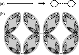
Figure 1: (a) Construction of the hierarchical lattice. (b) The lattice after $t=4$ steps in the construction. Communities at the $n=0,1,2$ levels of the hierarchy are shown with white, dark gray, and light gray backgrounds respectively.

II.2 Topological characteristics

Size of network: The total number of sites $N=\frac{2}{3}(4^{t}+2)$, the total number of bonds $N_{b}=\frac{1}{3}(4^{t+1}-1)$, and the diameter of the network (the maximum possible shortest-path distance between any two sites) is $D=2^{t+1}-1$.

Degree distribution: The probability $P(k)$ of finding a node with degree $k$ is zero except for $k=2^{m}+1$ for some integer $m\geq 1$, where $P(k)=3\cdot 4^{-m}$. The scale-free exponent $\gamma$ is calculated from the cumulative distribution $P_{\text{cum}}(k)\equiv\sum_{k^{\prime}=k}^{\infty}P(k^{\prime})\sim k^{1-\gamma}$. For large $k$ we find $P_{\text{cum}}(k)\approx k^{-2}$, so $\gamma=3$.

Community structure: We can define several levels of hierarchical modular organization, labeled by integer $n$: at the lowest level ($n=0$) we have clusters of solid bonds (shown with white background in Fig. 1(b)), with the dashed bonds acting as inter-community links; at the next level $(n=1)$ we can group together those communities which correspond to a single solid-bond cluster at the $(t-1)$th construction step (dark gray background in the figure); the $n=2$ level communities are outlined in light gray. In general, for a lattice after $t$ construction steps, a community at the $n$th level of the hierarchy evolved from a single solid-bond cluster at step $t-n$.

Fractal scaling: Adapting the analysis in Refs. Song1 ; Song2 , we can characterize the fractal topology of the network through two exponents $d_{B}$, $d_{k}$, defined as follows. At the $n$th level, all communities have the same diameter, $\ell_{B}=2^{\,n+2}-2$ (for $n<t-1$). Thus at each level the communities form a “box covering” of the entire network with boxes of the same $\ell_{B}$. The scaling of the number of boxes $N_{B}(\ell_{B})$ required to cover the network for a given $\ell_{B}$ defines the fractal dimension $d_{B}$, namely $N_{B}(\ell_{B})/N\sim\ell_{B}^{-d_{B}}$. In our case we have $N_{B}(\ell_{B})/N=4^{-n-1}\approx 4\ell_{B}^{-2}$ for large $n$, yielding $d_{B}=2$. Similarly the degree exponent $d_{k}$ of the boxes is defined through $k_{B}(\ell_{B})/k_{\text{hub}}\sim\ell_{B}^{-d_{k}}$, where $k_{B}(\ell_{B})$ is the number of outgoing links from the box as a whole, and $k_{\text{hub}}$ the degree of the most connected node inside the box. For boxes with large $k_{\text{hub}}$ we get a scaling $k_{B}(\ell_{B})/k_{\text{hub}}\approx 2\ell_{B}^{-1}$, giving $d_{k}=1$. As with all the real-world fractal networks examined in Refs. Song1 ; Song2 , the scale-invariance of the probability distribution is related to the fractal scaling of the network through the exponent relation $\gamma=1+d_{B}/d_{k}$, which is satisfied for $d_{B}=2$, $d_{k}=1$, and $\gamma=3$.

Modularity: The strength of community structure—the extent to which nodes inside communities are more tightly knit than an equivalent random network model—is quantified through the modularity NewmanGirvan $Q=\sum_{s}\left[l_{s}/N_{b}-(d_{s}/2N_{b})^{2}\right]$, where the sum runs over all communities, and $l_{s}$, $d_{s}$ are the total number of bonds and total sum of node degrees for the $s$th community. In our case each level $n$ in the hierarchy describes a different partition of the network into communities, and we find the corresponding modularity $Q=1-4^{-n-1}$. Thus $Q$ increases from $3/4$ at $n=0$ to the maximum possible value 1 as $n\to\infty$, showing that the modular structure becomes ever more pronounced as we go to higher levels.

Distribution of shortest-paths: We define $N_{\ell}$ as the total number of site pairs $(i,j)$ whose shortest-path distance along the lattice $\ell_{ij}=\ell$. The distance $\ell$ can take on values between 1 and $D$. $N_{\ell}$ has a non-trivial dependence on $\ell$, but satisfies the scaling form $N_{\ell}=2^{3t}f_{t}(\ell/D)$, where the function $f_{t}(\ell/D)$ approaches 0 for $\ell$ close to $1$ or $D$, and $f_{t}(\ell/D)\sim\text{O}(10^{-1})$ for $1\ll\ell\ll D$. The average shortest-path length $\bar{\ell}=\frac{2}{N(N-1)}\sum_{\ell=1}^{D}\ell N_{\ell}\sim D\sim N^{1/2}$, so the network is not small-world.

III Ising Model on the Network

III.1 Renormalization-group transformation

Let us now turn to the Hamiltonian for our system,

$$-\beta{\cal H}=J\sum_{\langle ij\rangle_{s}}s_{i}s_{j}+K\sum_{\langle ij\rangle_{d}}s_{i}s_{j}+H\sum_{i}s_{i}\,,$$ (1)

where $s_{i}=\pm 1$, $J,K>0$, and $\langle ij\rangle_{s}$, $\langle ij\rangle_{d}$ denote sums over nearest-neighbor pairs on the solid and dashed bonds respectively. The ratio of inter- to intra-community coupling is parametrized by $K/J$. The RG transformation is the reverse of the construction step: the two center sites in every cluster like the one on the right of Fig. 1(a) are decimated, giving an effective interaction between the two remaining sites. The renormalized Hamiltonian $-\beta{\cal H}^{\prime}$ has the same form as Eq. (1), but with interaction constants $J^{\prime},K^{\prime},H^{\prime}$. Two additional terms also appear: a magnetic field counted along the solid bonds, $H_{B}^{\prime}\sum_{\langle ij\rangle_{s}}(s_{i}+s_{j})$, and an additive constant per solid bond $G^{\prime}$. The renormalized interaction constants are given by:

$$\begin{split}J^{\prime}&=(1/4)\ln\left(R_{1}R_{2}/R_{3}^{2}\right),\quad K^{\prime}=K,\quad H^{\prime}=H,\\ H_{B}^{\prime}&=(1/4)\ln\left(R_{1}/R_{2}\right),\quad G^{\prime}=(1/4)\ln\left(R_{1}R_{2}R_{3}^{2}\right),\end{split}$$ (2)

where:

$$\begin{split}R_{1}&=w^{-4}xy^{-2}+2x^{-1}z^{4}+w^{4}xy^{2}z^{8},\\ R_{2}&=w^{-4}xy^{2}+2x^{-1}z^{-4}+w^{4}xy^{-2}z^{-8},\\ R_{3}&=x^{-1}w^{-4}+x^{-1}w^{4}+xy^{-2}z^{-4}+xy^{2}z^{4},\end{split}$$ (3)

and $w=e^{J}$, $x=e^{K}$, $y=e^{H}$, $z=e^{H_{B}}$. Under renormalization a nonzero site magnetic field $H$ induces a bond magnetic field $H_{B}$, while $H^{\prime}=H$ since the site field at the edge sites in each cluster is unaffected by the decimation of the center sites BOP . This transformation is exact, preserving the partition function $Z^{\prime}=Z$, and we iterate it to obtain the RG flows, yielding the global phase diagram of the system. Thermodynamic densities, corresponding to averages of terms in the Hamiltonian, transform under RG according to a conjugate recursion relation BOP . Iterating this along the flow trajectories until a fixed point is reached, we can directly calculate the magnetization $M=\frac{1}{N}\sum_{i}\langle s_{i}\rangle$, internal energy per site $U=\frac{1}{N}\langle\cal H\rangle$, and their derivatives $\chi=\frac{\partial M}{\partial H}$, $C=\frac{\partial U}{\partial T}$.

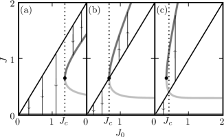
Figure 2: Renormalization-group flows in the closed subspace $H=H_{B}=0$ for three cases of the inter-community coupling strength $K/J$: (a) $K/J=0.75$, below the threshold value $(K/J)_{m}=\ln\left(\frac{1}{11}(43+24\sqrt{3})\right)/\ln(2+\sqrt{3})\approx 1.549$; (b) $K/J=(K/J)_{m}$; (c) $K/J=3>(K/J)_{m}$. In each case, the diagonal straight line represents the initial condition $J=J_{0}=1/T$, the thin vertical lines with arrows are sample flows, and the thick gray lines represent fixed points, with dark gray corresponding to stable fixed points, and light gray corresponding to unstable fixed points. The point where the light and gray curves meet is marginally stable. The dashed line marks the critical $J_{c}$ separating the disordered phase, flowing to the phase sink $J^{\ast}=0$, and the algebraically ordered phase, flowing to a line of finite temperature fixed points $J^{\ast}(J_{0})$ (the dark gray curve).

We are also interested in the pair correlation $G_{ij}=\langle s_{i}s_{j}\rangle-\langle s_{i}\rangle\langle s_{j}\rangle$ for arbitrary sites $i$, $j$ in the network. Since our lattice is highly inhomogeneous, $G_{ij}$ is not a simple function of $\ell_{ij}$. However, following the analysis in Ref. Dorogov1 , we can define an average correlation $G(\ell)=\frac{1}{N_{\ell}}\sum_{\{(i,j):\ell_{ij}=\ell\}}G_{ij}$, where the sum is over all pairs $(i,j)$ satisfying $\ell_{ij}=\ell$. While $G(\ell)$ cannot be directly calculated from the RG flows, we can determine its long-distance scaling properties. Moreover, the average correlation for a certain subset of pairs in the lattice can be explicitly calculated: at the $n$th level of the hierarchy, let site $i$ be a hub of a community, and $j$ be a site at the very edge of the same community, separated by a distance $\ell_{n}=2^{n+1}-1$. Denote the average of $G_{ij}$ restricted to this subset as $G_{\text{hub}}(\ell_{n})$. After $n$ RG steps, such pairs $(i,j)$ become nearest-neighbors along a solid bond, and thus we can obtain their thermodynamic average through the conjugate recursion relation BOP . The number of such pairs is $2^{2t-2n-1}$. For $1\ll\ell_{n}\ll D$, compared to the overall number of pairs with the same separation, $N_{\ell_{n}}\sim 2^{3t}$, the subset forms a vanishingly small fraction of the total in the $t\to\infty$ limit.

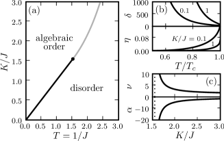
Figure 3: (a) Phase diagram. The black and gray curves represent infinite- and second-order transitions respectively. (b,c) Critical exponents. The dotted line marks $(K/J)_{m}$.

III.2 Phase diagram and critical properties

Fig. 2 depicts various cases for the renormalization-group flows, and the corresponding phase diagram in terms of temperature $T=1/J$ versus $K/J$ at $H=0$ is shown in Fig. 3(a). The two phases, both with $M=0$, are (1) a disordered phase where pair correlations decay exponentially, $G(\ell)\sim\exp(-\ell/\xi)$ with a finite correlation length $\xi$; (2) a phase with algebraic order, $\xi=\infty$, characterized by power-law decay of correlations, $G(\ell)\sim\ell^{-\eta(T,K/J)}$. Since this latter phase flows under RG to a line of finite-temperature fixed points (the dark gray curves in Fig. 2), a different fixed point for every value of $T$ and $K/J$, we have a varying exponent $\eta(T,K/J)$. Fig. 3(b) plots $\eta$ for $K/J=0.1$ and $1$, and we note that $\eta\to 0$ for $T\to 0$, as the system asymptotically approaches true long range order at $T=0$. Strengthening inter-community coupling has a similar effect, with $\eta$ decreasing for larger $K/J$.

For $K/J$ below a threshold value $(K/J)_{m}\equiv\ln\left(\frac{1}{11}(43+24\sqrt{3})\right)/\ln(2+\sqrt{3})\approx 1.549$, the phase transition is infinite order: as $T\to T_{c}^{+}$ we have exponential singularities of the Berezinskii-Kosterlitz-Thouless Berezinskii ; KosterlitzThouless (BKT) form, just like in the $XY$ model. $\xi\sim e^{A/\sqrt{t}}$ and the singular part of the specific heat $C_{\text{sing}}\sim e^{-B/\sqrt{t}}$, where $t\equiv(T-T_{c})/T_{c}$ and the constants $A,B>0$. It is interesting to note that for $K/J=1$, our Hamiltonian can be mapped by duality transformation to the Ising model on the small-world hierarchical lattice of Ref. HinczewskiBerker (the $p=1$ lattice). On this dual network a similar BKT transition occurs, though with the algebraic order in the high temperature phase (much as the Villain version of the $XY$ model is dual to a discrete Gaussian model describing roughening, with the low and high-temperature properties reversed ChuiWeeks ). BKT singularities have also been observed in an Ising and Potts system on an inhomogeneous growing network Bauer ; Khajeh . For $K/J>(K/J)_{m}$, on the other hand, the phase transition is second-order: $\xi\sim t^{-\nu}$, $C_{\text{sing}}\sim t^{-\alpha}$ for exponents $\alpha$, $\nu$, plotted as a function of $K/J$ in Fig. 3(c). Thus with increasing $K/J$ the system almost looks like an ordinary second-order Ising transition: a critical $T_{c}$ below which we have something very close to long-range order, since $\eta$ is nearly zero.

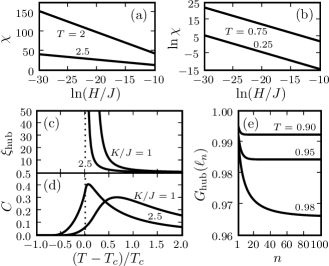
Figure 4: (a) Magnetic susceptibility $\chi$ at $K/J=1$ for $T=2,\,2.5>T_{c}$. (b) $\chi$ at $K/J=1$ for $T=0.75,\,0.25<T_{c}$. (c,d) Hub correlation length $\xi_{\text{hub}}$ and specific heat $C$ at $K/J=1,\,2.5$. (d) Hub correlation function $G_{\text{hub}}(\ell_{n})$, where $\ell_{n}=2^{n+1}-1$, at $K/J=1$ for $T=0.90,\,0.95,\,0.98<T_{c}$.

III.3 Griffiths singularities

The disordered phase in our network differs in one important aspect from a conventional paramagnetic phase: $M\sim H(1-\ln H)$ for small $H$, leading to a divergence in the susceptibility, $\chi\sim-\ln H$. We see this in Fig. 4(a) for $T=2$, $2.5$, and $K/J=1$. As mentioned above, the mechanism for this nonanalyticity at $H=0$ is similar to the one behind the Griffiths singularity in random ferromagnets. We can understand it through the distribution of Yang-Lee zeros YangLee of the partition function in the complex magnetic field plane. Introducing the variable $z=e^{-2H}$, the Yang-Lee theorem states that the zeros of $Z$ lie on the unit circle $z=e^{i\theta}$ in the complex $z$ plane. If $g(\theta)$ is the density of these zeros (a continuous distribution in the thermodynamic limit), then for a regular ferromagnet above $T_{c}$ we have $g(\theta)=0$ for a finite range of $\theta$ near the real axis $\theta=0$, so that $Z$ is analytic at $H=0$. However in our case $g(\theta)$ “pinches” the real axis: $g(0)=0$ but $g(\theta\neq 0)>0$. Since $g(\theta)$ is related to the magnetization through $g(\theta)=\frac{1}{2\pi}\lim_{r\to 1^{-}}\text{Re}\,M(z=re^{i\theta})$, we can deduce from the observed singularity that $g(\theta)\sim\theta$ for small $\theta$. The dominant contributions to this $g(\theta)$ come from large communities, centered at hubs with degree $k=2^{m}+1$ for $m\gg 1$, despite their small probability $P(k)=3\cdot 4^{-m}$.

We can see these contributions explicitly for the $K/J=0$ case, adapting arguments used to derive scaling forms for $g(\theta)$ in disordered ferromagnets BrayHuifang ; Chan . The system in this case is a disjoint set of solid-bond clusters, with the probability of a randomly chosen site being part of a cluster of size $N_{m}=2^{m-1}+1$ given by $P_{m}=3(2+2^{m})/2^{2m+1}$ (for $m\geq 2$). The average magnetization per site of such of cluster is easily calculated analytically, and takes the following approximate form for small $H$,

$$M_{m}\approx\tanh(Hf_{m}(J))\,,$$ (4)

where

$$\begin{split}&f_{m}(J)\\ &=1+\frac{N_{m}-1}{N_{m}}\tanh(2J)\left(2+(N_{m}-2)\tanh(2J)\right)\,.\end{split}$$ (5)

The $Hf_{m}(J)$ term in Eq. (4) can be interpreted as the effective field felt by the cluster, with the function $f_{m}(J)$ varying between $1$ at $J=0$ and $N_{m}$ at $J=\infty$. In the large $m$ limit $f_{m}(J)\to N_{m}\tanh^{2}(2J)$ for all $J>0$. To find $g_{m}(\theta)$, the cluster’s contribution to the overall $g(\theta)$, we plug in a small complex magnetic field $H=\frac{1}{2}(\epsilon-i\theta)$, corresponding to $z=(1-\epsilon)e^{i\theta}$, and take the real part of the resulting magnetization: $g_{m}(\theta)=\frac{1}{2\pi}\lim_{\epsilon\to 0}\text{Re}\,M_{m}(H=\frac{1}{2}(\epsilon-i\theta))$. This gives

$$g_{m}(\theta)=\lim_{\epsilon\to 0}\frac{1}{2\pi}\frac{\sinh(\epsilon f_{m}(J))}{\cos(\theta f_{m}(J))+\cosh(\epsilon f_{m}(J))}\,.$$ (6)

This expression is dominated by high, narrow peaks at $\theta=(2n+1)\pi/f_{m}(J)$, $n=0,1,\ldots$, and we can write it as a sum of delta functions in the small $\epsilon$ limit,

$$\begin{split}g_{m}(\theta)&\approx\lim_{\epsilon\to 0}\frac{1}{\pi}\sum_{n=0}^{\infty}\frac{\epsilon f_{m}(J)}{f_{m}^{2}(J)\left(\theta-\frac{(2n+1)\pi}{f_{m}(J)}\right)^{2}+\epsilon^{2}f_{m}^{2}(J)}\\ &=\sum_{n=0}^{\infty}\frac{1}{f_{m}(J)}\,\delta\left(\theta-\frac{(2n+1)\pi}{f_{m}(J)}\right)\,.\end{split}$$ (7)

Thus the total $g(\theta)$ for the system is

$$g(\theta)=\sum_{m=2}^{\infty}\sum_{n=0}^{\infty}\frac{P_{m}}{f_{m}(J)}\,\delta\left(\theta-\frac{(2n+1)\pi}{f_{m}(J)}\right)\,.$$ (8)

For small $\theta$, the nonzero contributions to $g(\theta)$ come from $m$ values where $f_{m}(J)=(2n+1)\pi/\theta$ for some $n$. Since $f_{m}(J)\approx N_{m}\tanh^{2}(2J)$ for large $m$, these are the contributions of clusters with large size $N_{m}\propto 1/\theta$, with a corresponding probability $P_{m}\approx 3/4N_{m}$. Eq. (8) becomes

$$g(\theta)\approx\sum_{m,n}\frac{3\theta^{2}\tanh^{2}(2J)}{4(2n+1)^{2}\pi^{2}}\,\delta\left(\theta-\frac{(2n+1)\pi}{N_{m}\tanh^{2}(2J)}\right)\,.$$ (9)

As $m\to\infty$ the delta function peaks become densely spaced, and from Eq. (9) it is evident for small $\theta$ that $g(\theta)$ scales like $g(b\theta)=bg(\theta)$ for any constant $b$, consistent with the observation of $g(\theta)\sim\theta$ deduced from the singularity in $M$. Thus we see this behavior is directly related to the presence of large communities around highly connected hubs, which have a scale-free distribution $P_{m}\sim N_{m}^{-1}$.

In comparison, for bond-diluted ferromagnets below the percolation threshold large connected clusters are exponentially rare, the resulting $g(\theta)\sim e^{-A(T)/|\theta|}$, and the Griffiths singularity is much weaker, leading to a finite $\chi$ at $H=0$ Harris . Turning now to the algebraic phase for $T<T_{c}$, here $M$ and $\chi$ behave as if at a critical point: $M\sim H^{1/\delta(T,K/J)}$, $\chi\sim H^{1/\delta(T,K/J)-1}$ as $H\to 0$. Fig. 4(b) shows $\chi$ for $K/J=1$, $T=0.75$, $0.25$, and Fig. 3(b) plots the exponent $\delta(T,K/J)$ for $K/J=0.1$ and $1$. The corresponding scaling of the density of zeros is $g(\theta)\sim\theta^{1/\delta(T,K/J)}$ near $\theta=0$.

III.4 Pair correlations

Finally, we consider the behavior of the hub correlation function $G_{\text{hub}}(\ell_{n})$. For $T>T_{c}$, we find an exponential decay with $\ell_{n}$, which we characterize by a correlation length $\xi_{\text{hub}}$. The divergence of $\xi_{\text{hub}}$ as $T\to T_{c}^{+}$ is shown in Fig. 4(c) for $K/J=1$, $2.5$. Like the overall pair correlation length $\xi$, $\xi_{\text{hub}}$ diverges with a BKT form for $K/J<(K/J)_{m}$ and as a power law for $K/J>(K/J)_{m}$. The onset of the rapid increase in $\xi_{\text{hub}}$ coincides with the position of the peak in the specific heat $C$, plotted in Fig. 4(d). Just like in the $XY$ model BerkerNelson , $C$ is smooth at $T_{c}$ for all $K/J$, and the peak occurs at $T>T_{c}$, corresponding to the onset of short-range order in the system. For $T<T_{c}$, $G_{\text{hub}}(\ell_{n})$ has a surprising behavior: as seen in Fig. 4(e), it approaches a nonzero limit as $\ell_{n}\to\infty$, a signature of long-range order. However, since $G_{\text{hub}}(\ell_{n})$ describes only a subset of pairs, a vanishingly small fraction of the total for large $\ell_{n}$, the long-range ordering of these pairs is compatible with $M$ being zero. The presence of such long correlations in the algebraic phase, and the overall slow power-law decay of $G(\ell)$ with $\ell$, is remarkable given that for “fat-tailed” scale-free networks (i.e. with $\gamma\leq 3$) pair correlations longer than nearest-neighbors are typically suppressed: one can prove that $G(\ell>1)=0$ at $H=0$ in the thermodynamic limit, if $\chi(H=0)$ is finite Dorogov1 . In our case $\chi(H=0)=\infty$ at all $T$, the proof does not apply, and we see that this fractal modular lattice is an important exception to the general expectation of weakened pair correlations on networks Dorogov1 .

IV Conclusions

In conclusion, we have introduced a hierarchical lattice network with the modular structure and fractal scaling characteristic of a wide array of real-world networks. The Ising model on this lattice—solved through an exact RG transformation—exhibits an interesting transition. A disordered phase with Griffiths singularities gives way at low temperatures to algebraic order: the system behaves as if at criticality for a broad range of parameters, and we find power-law decay of pair correlations, unexpected for this type of scale-free network.

The thermodynamic phenomena observed here are not confined to one particular network. In fact, we can consider the much larger class of hierarchical lattices that form scale-free networks on which the Ising model exhibits a standard order-disorder transition: these include fractal lattices on which Migdal-Kadanoff recursion relations are exact Migdal ; Kadanoff , related hybrid lattices Erbas , and their duals HinczewskiBerker2 . In all these cases we can modify the connected graph which defines the lattice construction step as follows: replace a subset of the bonds in the graph with dashed bonds (which remain unaltered as we iterate the construction) in such a way that the graph would break into two or more disjoint pieces if the dashed bonds were cut. The Ising model on the resulting hierarchical lattice will no longer flow under renormalization to an ordered fixed point at low temperatures, but rather to a continuous line of fixed points, yielding an algebraically ordered phase. And the power-law distribution of highly connected hubs in such networks will lead to Griffiths singularities in the disordered phase. Conversely the duals of such networks—which have infinite fractal dimension and show small-world scaling—have algebraic order at high temperatures. Recent studies have highlighted the diversity of structural properties in families of hierarchical lattice networks Rozenfeld ; Zhang —the ability to tune degree exponents, fractal dimensionality, and other topological aspects of these networks by varying the defining graph. The structural richness of these networks is manifested through unusual phase transitions and critical phenomena, already apparent even in a simple system like the Ising model. The use of renormalization-group methods to characterize cooperative behavior on this broad class of networks, both in the pure case and in the presence of bond randomness HinczewskiBerker , will be the subject of future work.

I thank A.N. Berker, T. Garel, and H. Orland for useful discussions.

References

- (1) M. Girvan and M.E.J. Newman, Proc. Natl. Acad. Sci. U.S.A. 99, 7821 (2002).
- (2) E. Ravasz, A.L. Somera, D.A. Mongru, Z.N. Oltvai, and A.-L. Barabási, Science 297, 1551 (2002).
- (3) M.E.J. Newman and M. Girvan, Phys. Rev. E 69, 026113 (2004).
- (4) F. Radicchi, C. Castellano, F. Cecconi, V. Loreto, and D. Parisi, Proc. Natl. Acad. Sci. U.S.A. 101, 2658 (2004).
- (5) C. Song, S. Havlin, and H.A. Makse, Nature 433, 392 (2005)
- (6) C. Song, S. Havlin, and H.A. Makse, Nature Physics 2, 275 (2006).
- (7) S.-H. Yook, F. Radicchi, and H. Meyer-Ortmanns, Phys. Rev. E 72, 045105(R) (2005).
- (8) A. Aleksiejuk, J.A. Hołyst, and D. Stauffer, Physica A 310, 260 (2002).
- (9) G. Bianconi, Phys. Lett. A 303, 166 (2002).
- (10) S.N. Dorogovtsev, A.V. Goltsev, and J.F.F. Mendes, Phys. Rev. E 66, 016104 (2002).
- (11) M. Leone, A. Vázquez, A. Vespignani, and R. Zecchina, Eur. Phys. J. B 28, 191 (2002).
- (12) F. Iglói and L. Turban, Phys. Rev. E 66, 036140 (2002).
- (13) A.V. Goltsev, S.N. Dorogovtsev, and J.F.F. Mendes, Phys. Rev. E 67, 026123 (2003).
- (14) J.O. Indekeu, Physica A 333, 461 (2004).
- (15) C.V. Giuraniuc, J.P.L. Hatchett, J.O. Indekeu, M. Leone, I. Pérez Castillo, B. Van Schaeybroeck, and C. Vanderzande, Phys. Rev. Lett. 95, 098701 (2005).
- (16) C.V. Giuraniuc, J.P.L. Hatchett, J.O. Indekeu, M. Leone, I. Pérez Castillo, B. Van Schaeybroeck, and C. Vanderzande, Phys. Rev. E 74, 036108 (2006).
- (17) K. Suchecki and J.A. Hołyst, Phys. Rev. E 74, 011122 (2006).
- (18) A.N. Berker and S. Ostlund, J. Phys. C 12, 4961 (1979).
- (19) M. Kaufman and R.B. Griffiths, Phys. Rev. B 24, 496 (1981)
- (20) M. Kaufman and R.B. Griffiths, Phys. Rev. B 30, 244 (1984).
- (21) A.-L. Barabási, E. Ravasz, and T. Vicsek, Physica A 299, 559 (2001).
- (22) F. Comellas and M. Sampels, Physica A 309, 231 (2002).
- (23) E. Ravasz, A.-L. Barabási, Phys. Rev. E 67, 026112 (2003).
- (24) J.S. Andrade, Jr., H.J. Herrmann, R.F.S. Andrade, and L.R. da Silva, Phys. Rev. Lett. 94, 018702 (2005).
- (25) J.P.K. Doye and C.P. Massen, Phys. Rev. E 71, 016128 (2005).
- (26) Z. Zhang, L. Rong, and S. Zhou, cond-mat/0512145.
- (27) Z. Zhang, F. Comellas, G. Fertin, and L. Rong, J. Phys. A: Math. Gen. 39, 1811 (2006).
- (28) Z. Zhang, L. Rong, and C. Guo, Physica A 363, 567 (2006).
- (29) Z. Zhang, L. Rong, and S. Zhou, Phys. Rev. E 74, 046105 (2006).
- (30) Z. Zhang, S. Zhou, and Z. Shen, cond-mat/0612624.
- (31) S.N. Dorogovtsev, A.V. Goltsev, and J.F.F. Mendes, Phys. Rev. E 65, 066122 (2002).
- (32) M. Hinczewski and A.N. Berker, Phys. Rev. E 73, 066126 (2006).
- (33) H. Rozenfeld, S. Havlin, and D. ben-Avraham, cond-mat/0612330.
- (34) Z. Zhang, S. Zhou, and T. Zou, cond-mat/0612427.
- (35) R.B. Griffiths, Phys. Rev. Lett. 23, 17 (1969).
- (36) S.R. McKay and A.N. Berker, Phys. Rev. B 29, 1315 (1983).
- (37) S.N. Dorogovtsev, A.V. Goltsev, and J.F.F. Mendes, Phys. Rev. E 72, 066130 (2005).
- (38) V.L. Berezinskii, Sov. Phys. JETP 32, 493 (1971).
- (39) J.M. Kosterlitz and D.J. Thouless, J. Phys. C 6, 1181 (1973).
- (40) S.T. Chui and J.D. Weeks, Phys. Rev. B 14, 4978 (1976).
- (41) M. Bauer, S. Coulomb, and S.N. Dorogovtsev, Phys. Rev. Lett. 94, 200602 (2005).
- (42) E. Khajeh, S.N. Dorogovtsev, and J.F.F. Mendes, cond-mat/0701156.
- (43) C.N. Yang and T.D. Lee, Phys. Rev. 87, 404 (1952); 87, 410 (1952).
- (44) A.J. Bray and D. Huifang, Phys. Rev. B 40, 6980 (1989).
- (45) P.Y. Chan, N. Goldenfeld, and M. Salamon, Phys. Rev. Lett. 97, 137201 (2006).
- (46) A.B. Harris, Phys. Rev. B 12, 203 (1975).
- (47) A.N. Berker and D.R. Nelson, Phys. Rev. B 19, 2488 (1979).
- (48) A.A. Migdal, Zh. Eksp. Teor. Fiz. 69, 1457 (1975) [Sov. Phys. JETP 42, 743 (1976)].
- (49) L.P. Kadanoff, Ann. Phys. (N.Y.) 100, 359 (1976).
- (50) A. Erbaş, A. Tuncer, B. Yücesoy, and A.N. Berker, Phys. Rev. E 72, 026129 (2005).
- (51) M. Hinczewski and A.N. Berker, Phys. Rev. B 72, 144402 (2005).