Magnetization dynamics in the single-molecule magnet Fe₈ under pulsed microwave irradiation

Abstract

We present measurements on the single molecule magnet Fe₈ in the presence of pulsed microwave radiation at 118 GHz. The spin dynamics is studied via time resolved magnetization experiments using a Hall probe magnetometer. We investigate the relaxation behavior of magnetization after the microwave pulse. The analysis of the experimental data is performed in terms of different contributions to the magnetization after-pulse relaxation. We find that the phonon bottleneck with a characteristic relaxation time of $\sim 10-100$ ms strongly affects the magnetization dynamics. In addition, the spatial effect of spin diffusion is evidenced by using samples of different sizes and different ways of the sample’s irradiation with microwaves.

I Introduction

Single molecule magnets (SMMs) have attracted much interest in recent years because of their unique magnetic properties. Having a regular structure, a well defined spin ground state and magnetic anisotropy they exhibit quantum phenomena even at macroscopic scales.novak:1995 ; friedman:1996 ; thomas:1996 Features such as quantum tunneling between spin states, interference between tunneling paths or blocking of the spin orientation at very low temperature show the quantum nature of SMMs. barco:2004 ; sorace:2003 ; wernsdorfer:science1999 ; wernsdorfer:2002a ; wernsdorfer:2000 In addition SMMs are supposed to be good candidates for data storage or quantum computing. leuenberger:2001

Recent works in the field of SMMs focused on spin dynamics and interactions with millimeter-wave radiation. The aima are to control the spin orientation in the sample and to selectively induce transitions between spin states. The crucial point for any application of SMMs is the knowledge of the spin relaxation time and the spin decoherence time. Therefore, various experiments have been performed in studying spin dynamics in SMMs in the presence of microwaves. Most measurements are based on standard electron paramagnetic resonance (EPR) techniques zipse:2003 or on optical spectroscopy mukhin:2001 , while others are based on magnetization measurements of the sample. In measuring the absorption of the microwaves via the decrease of magnetization we can obtain information about both the magnetization of the sample and EPR-like spectra. This technique also allows the precise control over the excitation of the sample and makes it possible to quantify the nonresonant heating.petukhov:2005 The magnetization sensor can be either a Hall magnetometer sorace:2003 ; bal:epl2005 , a micrometer sized superconducting quantum inference device (SQUID) wernsdorfer:2004 , a standard SQUID cage:2005 or an inductive pickup loop bal:2004 . Differences in these techniques lie mainly in the rapidity and sensitivity of the measurement, in the possibility of applying magnetic fields, and in the compatibility with microwaves.

In this paper we study the spin dynamics of the single-molecule magnet $Fe_{8}O_{2}(OH)_{12}(tacn)_{6}$, hereafter called Fe₈. This molecule contains eight Fe(III) ions with spins s=5/2. These spins are strongly superexchange coupled forming a spin ground state $S=10$ and the spin dynamics can be described assuming the giant spin model by an effective Hamiltonian barra:1996

$$\mathcal{H}=-DS_{z}^{2}+E(S_{x}^{2}-S_{y}^{2})+\mathcal{O}(4)-g\mu_{B}\vec{S}\cdot\vec{H}$$ (1)

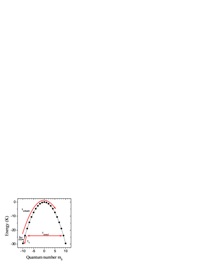
Figure 1: Spin states and energy barrier of the Fe₈ system. For an excited spin there are various processes relevant for spin dynamics.

$\vec{H}$ is the applied magnetic field, $\mathcal{O}(4)$ contains fourth order terms of spin operators and $g\approx 2$ represents the gyromagnetic factor. The anisotropy parameters $D=0.275$ K and $E=0.046$ K have been determined by various experimental methods. wernsdorfer:science1999 Classical EPR techniques, frequency domain magnetic resonance spectroscopy and neutron spectroscopy are complementary methods and give similar results. barra:1996 ; mukhin:2001 ; caciuffo:1998 ; park:2002 The nondiagonal terms in the Hamiltonian are responsible for the tunneling processes between spin states, whereas $D$ defines the anisotropy barrier of approximately 25 K as can be seen in Fig. 1.

In terms of the spin dynamics the giant spin model reveals various relaxation processes that are important for the evolution of the spin system in the time domain. As sketched in Fig. 1 the main parameters of the spin system are the spin relaxation time $\tau_{1}$ (time scale $\sim 10^{-7}~{}s$), the excitation over the barrier by a thermally activated multistep Orbach process with time constant $\tau_{orbach}$ (time scale $\sim 10^{-8}~{}s\times e^{\Delta E/k_{\rm B}T}$) where $\Delta E$ is the barrier height) and the tunnel probability between degenerated states with time constant $\tau_{tunnel}$ (time scale $\sim 10^{4}~{}s$ for the ground state tunneling).barra:1996 ; sangregorio:1997 The use of a large crystal of the single molecule magnet Fe₈ and, in consequence, the interactions between molecules make it necessary to introduce spin-phonon and spin-spin interactions. Effects such as spin decoherence (typical time scale $\tau_{2}\sim 10^{-9}~{}s$), phonon bottleneck (typical time scale $\tau_{ph}\sim 10^{0}~{}s$) or spin diffusion ($\tau_{diff}$) have to be taken into account for a complete description of the spin dynamics.Chiorescu:PRL2000 ; abragam

In this paper, a series of measurements on the SMM Fe₈ is presented investigating the relaxation of magnetization on millisecond and microsecond scales. In Section II we describe the experimental setup and the various experimental conditions. In Section III we present the experimental data that will be discussed in Section IV. Finally in Section V, we give some concluding remarks.

II Experimental techniques

II.1 General setup

The measurements are performed using a commercial 16 T superconducting solenoid and a cryostat at low temperatures in the range of 1.4 K to 10 K with temperature stability better than 0.05 K. The magnetization of the Fe₈ sample is measured by a Hall magnetometer. The Hall bars were patterned by Thales Research and Technology (Palaiseau), using photolithography and dry etching, in a delta-doped AlGaAs/InGaAs/GaAs pseudomorphic heterostructure grown by Picogiga International using molecular beam epitaxy (MBE). A two-dimensional electron gas is induced in the 13 nm thick $In_{0.15}Ga_{0.85}As$ well by the inclusion of a Si delta-doping layer in the graded $Al_{x}Ga_{1-x}As$ barrier. All layers, apart from the quantum well, are fully depleted of electrons and holes. The two-dimensional electron gas density $n_{s}$ is about $8.9\times 10^{11}~{}cm^{-2}$ in the quantum well, corresponding to a sensitivity of about 700 $\Omega$/T, essentially constant under $-100~{}^{\circ}$C. The sample is placed on top of the 10 $\mu$m $\times$ 10 $\mu$m Hall junction with its easy axis approximately parallel to the magnetic field of the solenoid. The three samples used in our experiments (150 $\times$ 100 $\times$ 30 $\mu$m³, 160 $\times$ 180 $\times$ 100 $\mu$m³ and 680 $\times$ 570 $\times$ 170 $\mu$m³) are exposed to microwave radiation. Microwaves are generated by a continuous wave (cw), mechanically tunable Gunn oscillator with a nominal output power of 30 mW and a frequency range of 110 GHz to 119 GHz. Pulses are generated using a SPST fast PIN diode switch (switching time less of than 3 ns) triggered by a commercial pulse generator. An oversized circular waveguide of 10 mm diameter leads the microwaves into the cryostat. In some of our experiments we use transition parts from oversized circular-to-rectangular WR6 waveguides. In other experiments we use only a cylindrical cone as an end piece of the circular waveguide that is right in front of the irradiated sample. The different configurations of the coupling of the microwaves to the sample that are investigated and compared are explained in the next paragraph. The cryostat is filled with exchange gas that thermodynamically couples the sample to the bath and allows a rather fast heat exchange. As the signal of the Hall magnetometer is in the range of a few microvolts a low-noise preamplifier is used in order to increase the signal-to-noise ratio in the rather long coaxial cables. Finally, the signal acquisition is done by a fast digital oscilloscope having a bandwidth of 1 GHz and 10 G/s sample rate and is done by taking an average over typically 32 frames.

II.2 Coupling of the microwaves to the sample

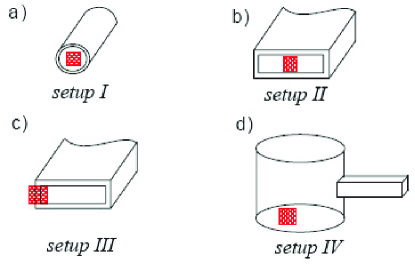
Figure 2: Different configurations of irradiating the sample with microwaves. We used several waveguides in order to change the electromagnetic environment of the sample, i.e. the coupling of the microwaves to the sample.

II.2.1 Conical waveguide

The simplest method of coupling microwaves to the sample is provided by a conical waveguide focusing microwaves from the oversized circular waveguide to the sample. In our experiments a cone with an opening of 4 mm in diameter is used. This setup is sketched in Fig. 2a and will be denoted hereafter as setup I. The conical waveguide has the advantage that it conserves the polarization of the passing light, thus allowing experiments depending on the angle of polarization or experiments with circularly polarized microwaves. Due to the large dimensions of the waveguide compared to the wavelength the propagation of the microwaves can be considered as quasioptical and the attenuation of microwave power is rather small.

II.2.2 Rectangular waveguide

Compared to the conical end piece of the waveguide a rectangular waveguide can focus the microwaves even better. The opening of a typical D-band WR6 waveguide is 1.7 mm $\times$ 0.8 mm, thus the cross section is nine times less than that in the case of the conical waveguide. However, the attenuation using the rectangular waveguide is fairly large, especially because of the transition part between oversized cylindrical and rectangular waveguides. At the end of the rectangular waveguide the field distribution is well defined. This feature allows us to irradiate the crystal in different ways. It can be put either in the central region of the waveguide (Fig. 2b, setup II), or at the edge of the waveguide, in order to partially irradiate the crystal (Fig. 2c, setup III). When irradiated partially, the magnetization of the crystal is measured with a Hall sensor at the nonirradiated side of the crystal. This method allows us to point out the importance of the inhomogeneous distribution of magnetization in the sample and spin diffusion processes that take place in large samples.

II.2.3 Microwave resonator

In some of our experiments a cylindrical cavity made of copper with detachable end plates is used, and the sample is placed on top of one of the end plates (Fig. 2d, setup IV). The inner diameter of the resonator is 10.10 mm and the height is 5.5 mm. A standard WR6 waveguide is coupled to the sidewall of the cavity by a coupling hole. The microwaves from the waveguide enter into the cavity at half height and can excite various modes obeying the selection rule $TE_{odd,*,*}$ and $TM_{even,*,*}$ (Table 1). All the modes have zero tangential electrical field on the end plates. The magnetic field has one or more maxima on the end plates according to the mode and the direction of the magnetic field is always radial. The sample is mounted on one of the end plates in such a way that the magnetic field in the cavity and the easy axes of the sample are parallel.

Resonator Mode	Frequency [GHz]
$TM_{413}$	108.631
$TE_{114}$	110.471
$TM_{014}$	111.436
$TM_{033}$	114.137
$TE_{314}$	116.097
$TM_{214}$	119.410
$TE_{124}$	120.176
$TM_{024}$	120.932

Table 1: Possible modes in a perfect cylindrical cavity in the range of 108 GHz to 121 GHz and for the dimension of the cavity specified in the text. Due to perturbations inside the cavity the calculated frequencies might differ from the theoretical ones.

By using a resonator we expect the amplitude of ac magnetic field to increase by a few orders of magnitude and thus allow better excitation of the sample even with very short pulses ($<$ 10 $\mu$s). The Q-factor for resonant modes is numerically calculated to be in the range of $10^{2}$ to $10^{3}$ depending on the mode. Therefore, the resonant modes are expected to have a full width at half maximum in the order of $0.1$ to $1$ GHz. Consequently we expect each mode to exist in a rather broad frequency band. The modes should be present in the resonator even when the microwave frequency does not exactly match the calculated resonance frequency.

In the experiments two slightly different end plates are used. In the first case an unprotected Hall bar with a sample on top is directly glued on top of the end plate. The position of the sample is about 2 mm off center of the end plate. In respect to the size of the cavity the Hall sensor and the sample represent a perturbation of the resonator that might be non-negligible. In consequence the frequencies for the different modes might slightly and inhomogeneously shift according to the calculated frequencies. Nevertheless the density of modes between 109 GHz and 120 GHz should remain rather high.

In the second case in order to perturb the cavity as weak as possible we protected the Hall bar with a copper foil. The position of the sample in this case is about 1 mm off center of the end plate. A small hole is drilled into the end plate and the Hall sensor is placed into the hole and is finally coated with a thin copper foil (thickness of 10 $\mu$m). Thus only the sample placed on the copper foil is directly exposed to the electromagnetic field inside the cavity whereas the Hall sensor and the cables are outside the resonator. In this setup the Hall sensor is protected from the microwave radiation by the thin copper foil, however the sensitivity in measuring the sample’s magnetization is expected to be weaker as in the unprotected case.

III Measurements

III.1 Magnetometry combined with microwaves

When the sample of SMM placed in the magnetic field $B$ is exposed to the cw microwaves, the magnetization curves show resonant absorption dips, similar to EPR spectroscopy spectra. The absorption of microwave radiation takes place at certain field values at a given frequency, when the microwave frequency matches the energy difference between two neighboring energy states, thus the allowed transitions are $\Delta m_{s}=\pm 1$. The populating of the upper levels (see Fig. 1) reduces the net sample’s magnetization $M$, the change of which $\Delta M$ can be detected via Hall voltage measurements. If the applied magnetic field is ramped while the microwaves are applied, the obtained magnetization spectra clearly show a series of nearly evenly spaced absorption dips, which can be easily attributed to the appropriate transitions, as shown in Fig. 3a by the thick solid curve. This curve is placed on the top of ”pure” magnetization curves, i.e. the curves measured without microwaves, depicted by the thin solid curves in Fig. 3a. These reference curves were measured at different cryostat temperatures in the range from 2 K (top curve) to 20 K (bottom curve) with 1 K incremental step. As can be seen from Fig. 3a, the 2 K magnetization data measured without microwaves and the magnetization data measured in the presence of microwaves do not match: the latter curve lies much below the first curve, as the temperature during the microwave experiment would be higher compared to that of the pure magnetization experiment. The difference between the two curves is denoted by the magnetization difference $\Delta M$, which is a good measure of the amount of microwave radiation absorbed by the spin system.

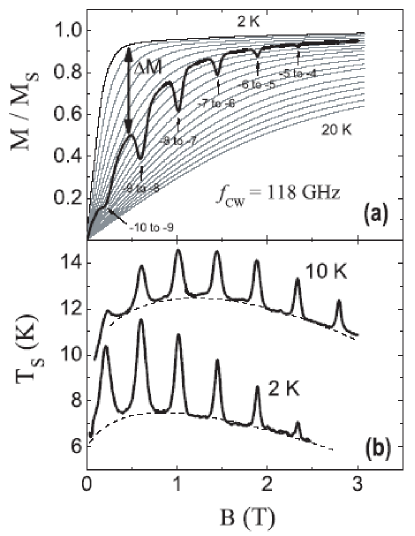
Figure 3: (a) Magnetization of Fe₈ as a function of magnetic field. The curves are normalized to the saturation magnetization value $M_{S}$. The thin solid curves represent the magnetization measured without microwaves at temperatures from 2 K to 20 K in 1 K steps. The thick solid curve represents magnetization curve in presence of cw microwaves of frequency $f_{CW}=118$ GHz measured at 2 K. The thick arrow represents the magnetization difference $\Delta M$ between data taken with and without microwaves at 2 K. (b) Spin temperature $T_{\rm S}$ vs applied field $B$, calculated using the mapping procedure described in the text. The dashed curves depict off-resonance absorption.

III.2 Spin temperature

Although the difference of magnetization $\Delta M$ can be used to qualify the amount of absorbed microwave photons, it is rather inconvenient to speak in terms of relative units of $\Delta M$. Another more significant complication in the use of $\Delta M$ for quantitative characterizations concerns the loss of sensitivity of $\Delta M$ close to zero field. As the magnetic field $B$ goes to zero, the magnetization also goes to zero, and hence the sensitivity of detection of absorption peaks goes to zero as well. Therefore, we need to perform a transformation of the magnetization to a physical quantity which does not depend on the magnetic field $B$.

Such a quantity called spin temperature was explicitly introduced in our earlier paper petukhov:2005 as a perfect measure of the amount of microwave radiation absorbed by an SMM spin system. The concept of spin temperature can be easily understood from Fig. 3a. We can map the magnetization curve (magnetization spectrum) obtained under the use of microwaves onto underlying reference magnetization curves, measured at different cryostat temperatures without microwaves. For each magnetization point of the absorption spectra one finds, at the corresponding field $B$, the temperature $T_{\rm S}$ that gives the same magnetization measured without microwave radiation [Fig. 3a]. The temperatures in between the reference magnetization curves are obtained with a linear interpolation. A typical result of such a mapping is depicted in Fig. 3b. $T_{\rm S}$ can be called the spin temperature because the irradiation time is much longer than the lifetimes of the energy levels of the spin system which were found to be around 10^-7 seconds Wernsdorfer:EPL2000 . The phonon relaxation time $\tau_{ph}$ from the crystal to the heat bath (cryostat) is much longer, typically between milliseconds and seconds Chiorescu:PRL2000 . The spin and phonon systems of the crystal are therefore in equilibrium.

Figure 3b shows spin temperature data calculated for the magnetization measurements at cryostat temperatures of 2 K and 10 K, performed at frequency of cw microwaves of $f_{CW}=118$ GHz. From Fig. 3b we can conclude that the obtained spin temperatures $T_{\rm S}$ are much larger than the cryostat temperature $T$. This is associated with a strong heating of the spin system. This effect is more prominent at lower $T$: the baseline of 2 K $T_{\rm S}$ spectrum is around 7 K, while 10 K $T_{\rm S}$ spectrum’s background is very close to the nominal cryostat temperature $T=10$ K, as depicted by the dashed curves in Fig. 3b. We also see that both backgrounds are not flat, but are magnetic field dependent. The presence of the spectra’s nonflat background is due the presence of off-resonance absorption of microwaves, which takes place between the resonant absorption peaks. The nonresonant (or background) absorption is modulated in the following way: it has larger contribution where the resonant absorption has larger spectral weight, i.e. higher peaks of $T_{\rm S}$. Interestingly, the off-resonance absorption was also evidenced in the EPR spectra of SMMs, but its origin remains undiscussed park:2002 ; Hill:PRB02 . On the top of the nonresonant background one can see a perfect EPR-like absorption spectra, and the $T_{\rm S}$ peak positions exactly match the magnetic field values, corresponding to $|\Delta m_{S}|=1$ transitions (see Fig. 3).

III.3 Pulsed microwave measurements

Another way to perform $\Delta M$ measurements in order to calculate the spin temperature $T_{\rm S}$ is to utilize a pulsed microwave (PW) radiation petukhov:2005 . This method gives direct information about $\Delta M$ at a given magnetic field value $B$, at a given temperature $T$, and at a given microwave power, a measure of which is a pulse length $t$. This advanced method also drastically reduces the heating of the sample with microwaves, since the repetition rate of microwave pulses (typically 200 ms in our experiments) is much larger than the pulse length values, typically $t\leq 10$ ms. Restoration of the after-pulse magnetization to the equilibrium value $M_{0}$ normally takes less than 100 ms, as can be seen in Fig. 4.

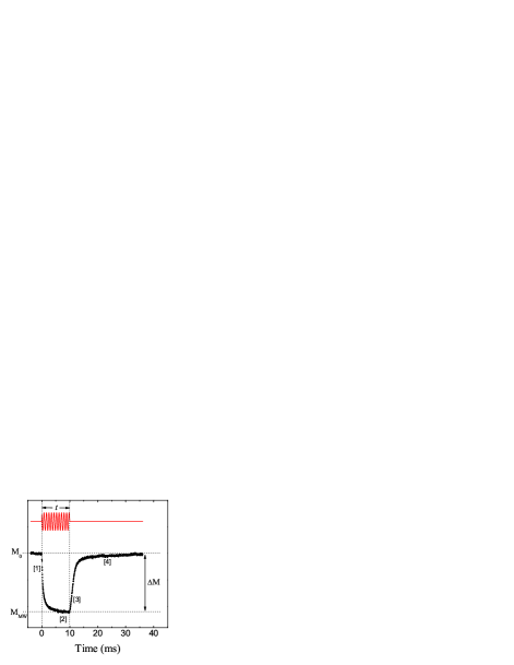
Figure 4: Typical oscillogram of a pulsed experiment. The magnetization was measured as a function of time for a microwave pulse length of $t=10$ ms at temperature $T$ = 10 K.

The scheme of possible pulsed experiment is depicted in Fig. 4. The top part of Fig. 4 schematically shows microwave pulse of duration $t=10$ ms, and the bottom part of the figure shows time-resolved development of magnetization data collected during such pulsed experiment. The magnetization before and at the end of the pulse has values $M_{0}$ and $M_{\rm MW}$, respectively. The difference between the unperturbed magnetization value $M_{0}$ and magnetization at the final edge of the pulse $M_{\rm MW}$ (i.e. the height of the magnetization response) $\Delta M=M_{\rm MW}-M_{0}$ is identical to the magnetization difference $\Delta M$ defined for the cw microwaves case, as graphically explained by Fig. 3a. Thus, having a set of reference magnetization curves, shown by thin curves in Fig. 3a, and magnetization difference $\Delta M$ defined from the PW measurements, as shown in Fig. 4, one can perform spin temperature $T_{\rm S}$ calculations. Such calculations for Fe₈ have been performed in our previous work for the PW configuration and it has been shown that obtained spin temperatures $T_{\rm S}$ are much closer to the cryostat temperature $T$ than that for cw experiments petukhov:2005 . The linewidths and shapes of PW $T_{\rm S}$ spectra depend on the pulse length, but in general the peak positions of cw and PW configurations are identical. In contrast to the cw experiments, the PW method can successfully resolve absorption peaks near zero field petukhov:2005 .

Unlike cw measurements, PW magnetization profiles contain information not only about $\Delta M$ but also about the magnetization dynamics. Let us assume that the applied magnetic field $B$ and the microwave frequency $f_{PW}$ do match the resonance condition, i.e., the in-resonance microwave pulse is applied. Since the sample’s magnetization is connected to the spin state level occupancy of SMMs, the magnetization dynamics should be connected to the level’s lifetime. The spin-spin relaxation time $\tau_{2}$ is usually much shorter than the spin-phonon relaxation time $\tau_{1}$; if $\tau_{1}$ obtained through magnetization dynamics is short enough, it can determine the upper limit of $\tau_{2}$. Finally, since there is an increase of the sample’s temperature due to the heating with microwaves, the phonon relaxation time $\tau_{ph}$ from the crystal to the heat bath (cryostat) can be systematically studied from the magnetization ”cooling” after long enough pulses in PW experiments. Thus, the detailed consideration of the time-resolved magnetization profile, depicted in Fig. 4, might provide information about the $\tau_{1}$, $\tau_{2}$, and $\tau_{ph}$ relaxation times.

Let us consider the magnetization behavior during a PW experiment in detail in Fig. 4. At the beginning of the pulse, the magnetization rapidly decreases (region [1]) and starts to saturate (region [2]) until the end of the pulse. We need to note that a complete saturation is observed only for rather long pulses of several seconds. After the microwave pulse is switched off, the magnetization restores back to the equilibrium value $M_{0}$. At the beginning of its restoration the magnetization increases rapidly (region [3]), several millisecond later magnetization increase changes to the slower behavior (region [4]), until it levels out at $M_{0}$. This slow restoration lasts long, up to a hundred of milliseconds, but we were able to follow it completely, since the typical repetition time of pulses was 200 ms. This brings us to the conclusion, that region [4] might comprise the information about the cooling of the sample after the microwave pulse, i.e. the phonon relaxation time $\tau_{ph}$ from the crystal to the heat bath (cryostat). Exactly this relaxation time is typically of the order of magnitude of several tens of milliseconds up to seconds Chiorescu:PRL2000 . The fast-running beginning of region [3] could contain the longitudinal relaxation time $\tau_{1}$ (typically $\sim 10^{-7}$ seconds Wernsdorfer:EPL2000 ). There was another interesting observation in region [3] of the magnetization curve in Fig. 4: during some of our experiments we have observed that right after the pulse was switched off the magnetization continued to decrease for some time and only then started to increase to the equilibrium value. Similar behavior of magnetization after microwave pulses in Fe₈ was observed in the recent work of Bal et al. bal:epl2005 . Below we will explicitly investigate such an overshooting of magnetization after the microwave pulse. In principle, regions [1] and [2] are very similar to the regions [3] and [4], correspondingly. The problem with the use of this part of magnetization evolution curve is that regions [1] and [2] are limited by the pulse duration, and therefore it seems to be problematic to estimate relaxation times from this part of the data, especially the long-lasting $\tau_{ph}$. In this paper, we pay attention to the time-resolved behavior of the magnetization after the pulse in a PW experiment, i.e. to regions [3] and [4] as determined in Fig. 4.

III.4 The model

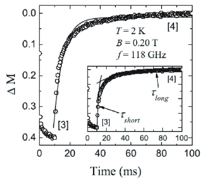
Figure 5: Fit of magnetization restoration data (open circles) with a single exponential relaxation (solid line). The inset shows the fit with two exponents: fast relaxation with relaxation time $\tau_{short}$ and cooling with relaxation time $\tau_{long}$. Note that the depicted magnetization data curve contains only 2% of the experimental points taken during the single experiment, i.e. only every 50th point is shown.

First, in order to analyze the behavior of the magnetization after the microwave pulse, we have tried to fit the magnetization data in regions [3] and [4] by a single exponential relaxation. We have found that in many cases a single exponential description was unsatisfactory, as shown in Fig. 5. This is not surprising in the framework of consideration concerning different relaxation times given above. Indeed, the $\tau_{1}$ relaxation time, which can be found right after the pulse is much shorter than the cooling $\tau_{ph}$ relaxation time, which can be a major contribution in the tail of magnetization restoration. Therefore, we have separately considered two different regions of the magnetization restoration curve, as depicted in the inset of Fig. 5. Firstly, we have assumed that the magnetization data, obtained right after the pulse was switched off (typically, within the time frame of 10-20% of the pulse length), could contain the information about the spin-lattice $\tau_{1}$ relaxation time. This data can be described by a fast exponential relaxation, and we will denote the corresponding relaxation time by $\tau_{short}$, as shown in the inset of Fig 5. Another valuable contribution to the overall magnetization restoration comes from the cooling of the specimen after the microwave pulse, such a process can be described by the long-lasting relaxation process with relaxation time $\tau_{long}$, taken later after the pulse was switched off (typically, 3 to 4 pulse length values later after the pulse edge until the end of the magnetization data), as depicted in the inset of Fig 5. If the slow relaxation $\tau_{long}$ is responsible for the sample’s cooling, it can only be sensitive to the sample size and its thermal coupling to the bath, with both parameters unchanged during an experimental set. Therefore, we expect this contribution to be temperature and pulse length independent. Nevertheless, the slow relaxation $\tau_{long}$ contribution (i.e. sample thermalization) can become dominating over the fast relaxation $\tau_{short}$ on increase of the temperature and/or for very long pulses, since the $\tau_{short}$ drastically shortens under such conditions and can be unresolved. In this case, a single exponential relaxation could be suitable for the magnetization data description and it could give solely the relaxation time $\tau_{long}$. In our experiments we avoid such a situation and we carefully adjust the experimental condition to have two clearly distinguishable regions [3] and [4], where the uncontroversial analysis by means of $\tau_{short}$ and $\tau_{long}$ can be performed. This analysis was applied in the following magnetization relaxation measurements.

III.5 Relaxation of magnetization

We have studied the relaxation of magnetization employing different sample irradiation configurations, described in the ”Experimental setup” part. In all the cases, the applied magnetic field was set to 0.2 T and the frequency of microwaves during pulses was 118 GHz. Thus, below we describe the studies of the magnetization dynamics of the first transition from the ground state $m_{S}=-10$ to the first excited state $m_{S}=-9$, since the given magnetic field and frequency values match the resonance condition for Fe₈ placed into magnetic field along its easy axis petukhov:2005 . While the temperature and the pulse length were changed during the PW experiments, shown below, the repetition time of microwave pulses was always set to 200 ms.

III.5.1 Measurements with conical waveguide

Figure 6: Temperature dependence of relaxation time $\tau_{short}$ measured for a small sample with a conical waveguide. The microwave pulses of repetition time of 200 ms and of different lengths were applied: 0.05 ms (dotted curve), 0.1 ms (solid curve), 0.5 ms (dashed curve), 1 ms (dashed-dotted curve), 5 ms (bold solid curve), and 10 ms (bold dashed curve). Color online.

Measurements with a conical waveguide are performed on a tiny sample placed in setup I configuration, as shown in Fig. 2a. The volume of the sample is 150 $\times$ 100 $\times$ 30 $\mu$m³. We have investigated the $\tau_{short}$ and $\tau_{long}$ relaxation times as a function of temperature $T$ for different values of pulse length. The results obtained from such PW experiments for the short relaxation time $\tau_{short}$ are depicted in Fig. 6.

The fast relaxation shows the relaxation time $\tau_{short}$ of the order of magnitude of 1-1.5 ms. The temperature dependence of $\tau_{short}$ is not strong, but is clearly pronounced: on warming from 2 K to approximately 4 K the relaxation time $\tau_{short}$ decreases, reaches its minimum near 4 K, and then smoothly increases on further warming (see Fig. 6). The decrease of relaxation time $\tau_{short}$ on warming from 2 K to approximately 4 K is much steeper for shorter pulses, while the $\tau_{short}$ behavior above 4 K is similar for all the pulse length values.

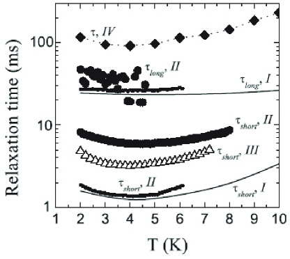
Figure 7: Generic plot depicting temperature dependence of fast relaxation time $\tau_{short}$ and slow relaxation time $\tau_{long}$ for different sample sizes and different sample’s irradiation configurations: setup I (solid curves), setup II for a big and a small sample (big and small solid circles, respectively), setup III (open triangles), and setup IV (solid rhombus with dotted curve). Note that the Latin numbers stand for corresponding setup notation.

For the same sample and experimental configuration setup I, the slow relaxation time $\tau_{long}$ is approximately one order of magnitude greater, that is, its value lies around 20 ms. This long-lasting relaxation time is temperature independent within 5% in the measured temperature range, as shown in Fig. 7, where both $\tau_{short}$ and $\tau_{long}$ obtained from the 10 ms data using setup I configuration are shown by solid curves for comparison. This behavior of $\tau_{long}$ perfectly fits into the above given explanation of $\tau_{long}$-process as a cooling of the sample after the microwave pulse. Such a cooling rate is only defined by the sample thermal coupling to the bath, and therefore, it is permanent for a given experimental setup.

Figure 7 shows the generic plot of relaxation times $\tau_{short}$ and $\tau_{long}$, obtained from all the experimental configurations at 10 ms pulse length over 200 ms pulse repetition time. Such a rather long pulse length was chosen mainly due to the following reasons. At first, at rather long pulses the contribution of the $\tau_{long}$-process, i.e. the sample thermalization after the pulse, becomes valuable, making better separation of $\tau_{short}$ and $\tau_{long}$ data intervals possible, and thus both fast and long relaxations can be estimated and compared for the same system under the same experimental condition. Secondly, at long pulses, a high signal-to-noise ratio enables better fitting, even for the limited regions of experimental data. Finally, as will be shown below, at such long pulses there are no overshooting phenomena observed for both small and big samples at all the temperatures applied; with the presence of overshooting, the analysis of magnetization data in terms of relaxation exponents becomes controversial.

III.5.2 Measurements with a rectangular waveguide

The irradiation of the sample with a piece of the rectangular waveguide WR6 is advantageous in the sense that the distribution of electromagnetic field is known at the waveguide cut edge. Another advantage of the use of the WR6 waveguide is that the area of its opening (1.36 mm²) is approximately 9 times smaller than the area of the 4 mm opening of the conical waveguide, so we could expect a higher density of microwaves exposed to the sample. On measurements employing rectangular waveguide, setup II configuration of irradiating the sample with microwave radiation is used. In this configuration, the sample is placed in the geometrical center of the waveguide opening, as schematically shown in Fig. 2b. Setup I configuration provides the point of maximal magnetic field for the propagating TE₁₀ mode in a rectangular waveguide poole .

In our magnetization study employing setup II configuration, we have used two samples of different volumes: a big sample with a volume 680$\times$570$\times$170 $\mu$m³ and a smaller sample with a volume of 160$\times$180$\times$100 $\mu$m³. We will refer these samples hereafter as big and small, correspondingly. The measurements were performed upon irradiation with pulsed microwaves of 118 GHz and at applied magnetic field of 0.2 T, these conditions correspond to the first transition from the ground state -10 $\rightarrow$-9 for Fe₈ system along the easy axis. We have found that the relaxation time $\tau_{short}$ for the small sample behaves very similar to the relaxation time $\tau_{short}$ of the sample used with setup I. Indeed, this relaxation time decreases during the temperature increase from 2 K to 4 K, where it reaches its minimal value of around 1.5 ms, as shown by the small solid circles in Fig. 7. On the consequent increase of the temperature above 4 K, we see the increase of $\tau_{short}$ with temperature $T$. The $T$-dependence of the fast relaxation parameter $\tau_{short}$ for the big sample is qualitatively similar to that of the small sample, the corresponding data is depicted with big solid circles in Fig. 7. Here, the relaxation time also reveals a minimum at around 4 K, but the absolute values of $\tau_{short}$ for the big sample are approximately four times higher, and both dependences can be perfectly scaled one onto another. The $\tau_{long}$ values for both the small and big samples are shown in Fig. 7 by the small and big solid circles, respectively; both these relaxation times lie around 25-30 ms and they are temperature independent, similar for the earlier described configuration setup I. This is not surprising, since in both configurations of coupling of the samples to the electromagnetic (EM) radiation, the surrounding of the sample was the same: we have used the same sample holder in both cases, and the same amount of exchange gas was contained in the sample volume chamber for the sample’s thermalization. This was not the case when the sample was placed onto the interior wall of the massive copper cavity resonator.

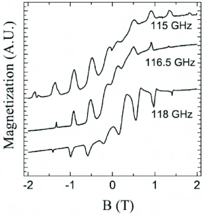
Figure 8: Magnetization loops measured at several cw microwave frequencies using a cavity. Note, that the curves are equally scaled.

III.5.3 Measurements with a cavity

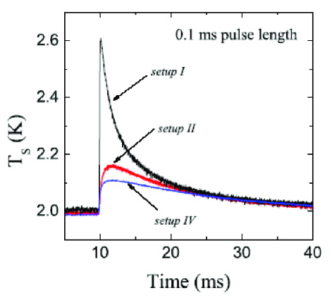
Figure 9: Spin temperature calculated during a pulse of length of 0.1 ms at nominal cryostat temperature $T=2$ K for the different ways of irradiating sample with microwaves. Color online.

In order to increase the amplitude of the EM radiation exposed to the sample, we have used the cylindrical copper cavity resonator, construction details of which are given above. The corresponding configuration is denoted as setup IV and it is shown in Fig. 2c. The use of a microwave cavity assumes the use of different modes compatible with the cavity geometry and the microwave frequency. The general problem of the cavity usage is that the modes of the cavity are coupled to the sample in a different way, i.e. the electromagnetic environment of the sample inside the cavity is strongly dependent on the mode and the frequency. This leads not only to different amplitudes of exposed (and therefore, absorbed) microwaves, but also to the irregularities of the absorption spectra. Figure 8 shows the microwave absorption spectra of magnetization obtained at several frequencies, separated just 1.5 GHz from each other; the spectra are obtained by the use of cw microwaves with setup IV. The sample used for the studies with the cavity has dimensions of 680$\times$570$\times$170 $\mu$m³. Unfortunately, when a smaller sample is used in the cavity-employed configuration setup IV, the sensitivity is reduced drastically. This is due to the fact that the sample’s change of magnetization is sensed by the Hall bar separated by a copper foil, as described above.

It can be seen that the modes differ not only in the amplitude of absorption peaks, but some of them are also highly distorted (peaks instead of dips, amplitude-phase mixing, asymmetry for opposite field directions). For the magnetization relaxation measurements we choose the frequency of 118 GHz, since the mode working at this frequency shows the largest amplitudes of absorption peaks in the positive magnetic-field direction; so, all the measurements presented below are taken at the frequency of 118 GHz.

In general, we find that there is no increase of the EM-field amplitude exposed on the sample in comparison with the case, when the sample is irradiated with microwaves without a cavity. The best way to quantitatively characterize the amount of EM radiation (photons) absorbed by the sample is to consider the spin-temperature $T_{\rm S}$ growth due to the exposure of a microwave pulse. Using the mapping procedure described above, we convert the magnetization data obtained at a pulse length of 0.1 ms into $T_{\rm S}$ for the different configurations of coupling of the sample to the microwaves. The plot, representing spin temperature $T_{\rm S}$ calculated when no cavity is used (setup I and setup II) and in cavity-employed configuration (setup IV), is depicted in Fig. 9. The plot presented in Fig. 9 shows no evidence of enhancement of absorption of microwaves, when the resonant cavity is used, although the best performing mode is chosen for this spin temperature comparison. Instead, both waveguide-employed configurations clearly show a better performance. The same sample is used for setup II and setup IV configurations, while the smaller sample is used in configuration setup I; details of the sample’s size are given above.

The use of a cavity also significantly extends the relaxation of magnetization after the microwave pulse. This slowing of magnetization restoration is also clearly visible from the spin-temperature dynamics, shown in Fig. 9, as compared to the experiment without a cavity setup II on the same sample. We have summarized the relaxation parameters when the cavity was used on the generic plot shown in Fig. 7 and compared these relaxation time values to the parameters, obtained from the magnetization restoration during pulsed microwave measurements on the same sample without cavity. The relaxation time data obtained during cavity-employed experiment are denoted as ”$\tau$, IV” on Fig. 7. The obtained relaxation time $\tau$ is around 100-200 ms, which is one order of magnitude larger than the slow relaxation time $\tau_{2}$, obtained in no-cavity experiments. We cannot unambiguously attribute the obtained relaxation time $\tau$ to the fast relaxation $\tau_{short}$, although the data for its calculation were taken right after the pulse, as what was done for the $\tau_{short}$ definition in no-cavity setups. We think that the calculated relaxation time $\tau$ rather corresponds to the mixture of $\tau_{short}$ and cooling of the sample thermally coupled to the massive copper cavity, i.e. the relaxation time $\tau_{long}$.

III.5.4 Background absorption

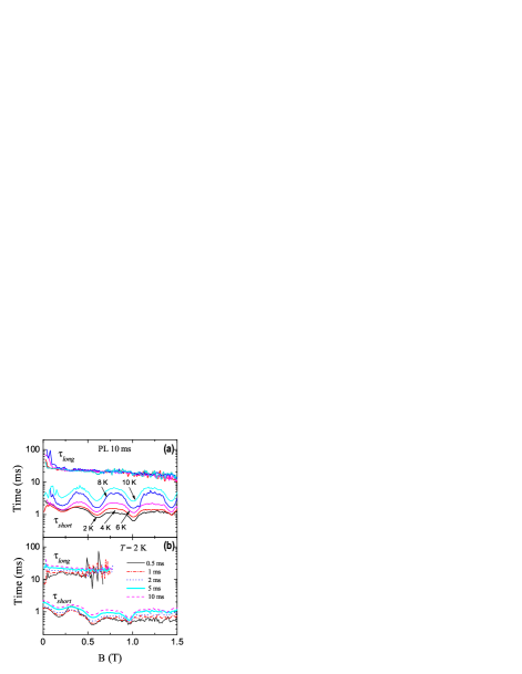
Figure 10: (a) Relaxation time $\tau_{short}$ and $\tau_{long}$ as a function of applied magnetic field in PW measurements of pulse length of 10 ms and frequency $f=118$ GHz. The measurements were performed using setup I at several temperatures. (b) Relaxation time $\tau_{short}$ and $\tau_{long}$ as a function of applied magnetic field at temperature $T=2$ K and frequency $f=118$ GHz. The measurements were performed using setup I at several pulse length values: 0.5 ms (solid curve), 1 ms (dotted-dashed curve), 2 ms (dotted curve), 5 ms (bold solid curve), and 10 ms (dashed curve). The repetition time of the pulses was 200 ms. Color online.

All the measurements, described above are performed at a resonance condition corresponding to the transition from the ground state, i.e. -10 $\rightarrow$ -9. At 118 GHz, a frequency which is used for current studies, the appropriate applied magnetic field is always set to 0.2 T, and thus the resonant condition is fulfilled for the Fe₈ system along the easy axis. Thus, only the resonant absorption is detected. Nevertheless, as we have mentioned above, there is also a significant off-resonant, or background, absorption.

In Fig. 10 we present the relaxation time $\tau_{short}$ and $\tau_{long}$ as a function of the applied magnetic field. The magnetic field is set in discrete steps from zero field to 1.5 T with an increment of 0.05 T. These relaxation times are calculated from the PW measurements performed using configuration setup I at several temperatures [Fig. 10a] and at several pulse length values [Fig. 10b].

Both figures show that the long relaxation time $\tau_{long}$ remains pulse length and field independent within the noise bandwidth and equals to approximately 25 ms; there is no resonance structure evidenced in $\tau_{long}$ field-dependence. This is consistent with our consideration of the slow relaxation as a cooling of the system. Note that above approximately 0.5 T the magnetization deviation amplitudes are reduced for short pulse values and the corresponding $\tau_{long}$ curves become very noisy in Fig. 10b.

$\tau_{short}$ follows the resonance behavior and clearly pronounced resonant dips can be seen in both figures. We see that off-resonance and in-resonance relaxation time $\tau_{short}$ values lie within the same order of magnitude (around 1-3 ms), while $\tau_{long}$ is one order of magnitude larger. For the pulse length value of 0.5 ms [Fig. 10b], the difference between the in-resonance value at $H=0.2$ T and the off-resonance value of $H=0.38$ T is a factor of 2, while for the pulses with a duration of 10 ms this factor is reduced to 1.2.

III.6 Magnetization overshooting

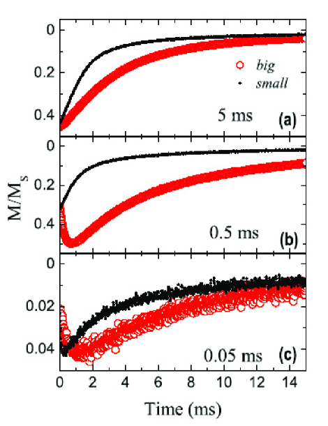
Figure 11: Typical plots of PW measurements of magnetization as a function of time performed on big (solid circles) and on small (open circles) samples. The data plotted are taken at 5 ms (a), 0.5 ms (b), and 50 $\mu$s (c) right after the microwave pulse was switched off. Color online.

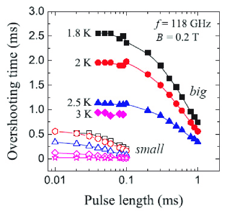
Figure 12: Position of the magnetization overshooting minima as a function of pulse length for the big (solid symbols) and for the small (open symbols) samples. The measurements were done at temperatures of 1.8 K (squares), 2 K (circles), 2.5 K (triangles), 3 K (diamonds), and 4 K (stars). Color online.

As we have mentioned above, in some of our PW experiments we observed an overshooting of the magnetization after the microwave pulse, when the magnetization continued to decrease even after the pulse is switched off. This phenomenon, for example, can be clearly seen in the magnetization data recalculated into spin temperature for setup II and setup IV, as shown in Fig. 9. A similar effect is also evidenced in the work of Bal et al. bal:epl2005 . Such an overshooting, however, is not observed in magnetization measurements employing setup I, where we have performed pulsed microwave experiments with pulses of the length of 10 ms down to 1 $\mu$s. Note that two different samples are used with setup II, and the volume of the small sample used in this study is approximately 6 times larger than the volume of the crystal, used in the measurement with setup I.

In measurements employing rectangular waveguide, two configurations setup II and setup III are possible. In the former configuration, the sample is placed in the geometrical center of the waveguide opening; in the latter configuration, the sample is placed at the midpoint of the shortest wall of the waveguide, as schematically shown in Fig. 2. Both configurations provide the points of maximal magnetic field for the propagating TE₁₀ mode in a rectangular waveguide poole . In setup II configurations, a sample of any size can be used, while only a sample of large enough volume can be used in setup III, because a tiny sample cannot be properly placed at the edge of the waveguide for partial irradiation with microwaves.

In order to find the nature of the overshooting of magnetization restoration after the microwave pulse, we employ setup III configuration, which allows partial irradiation of the sample with microwaves. We construct a sample holder, where setup II and setup III can be used simultaneously, i.e. two samples can be exposed to the microwaves at the same time. The change of each sample’s magnetization can be sensed by an individual Hall bar mounted underneath the sample.

For measurements we use two different size samples of Fe₈: one sample, hereafter referred to as small, had dimensions of 160$\times$180$\times$100 $\mu$m; and another sample, hereafter referred to as big, had dimensions of 680$\times$570$\times$170 $\mu$m. The small sample was placed in setup II and was entirely irradiated with microwave radiation. The big sample was placed in configuration setup III and only a part of it was exposed to the microwaves; the Hall bar was placed under the ”dark” part of the big sample. Both samples were mounted with their easy axes parallel to the direction of the applied magnetic field set to the value of 0.2 T, which corresponds to the first transition -10 $\rightarrow$ -9 at the frequency of 118 GHz.

The typical oscillograms of pulsed microwave measurements performed at temperature $T=2$ K and pulse durations of 5 ms, 0.5 ms, and 50 $\mu$s for the big and the small samples are presented in Fig. 11; and the data plotted are taken right after the microwave pulse was switched off. As seen in Fig. 11a, after rather long pulses of duration of 5 ms, no magnetization overshooting is observed for both the big and small samples. At ten times shorter pulse length of 0.5 ms, the magnetization restoration of the small sample reveals no overshooting feature, while the magnetization of the big sample continues to decrease, reaches the minimum at approximately 0.6 ms after the microwave pulse is switched off, and only then increases and saturates to the equilibrium value [see Fig. 11b]. When the microwaves are applied within the pulses of length of 50 $\mu$s, the magnetization data of the big sample show even more overshooting: the minimum of the magnetization curve is observed approximately 1.2 ms after the pulse edge, see Fig. 11c. At the same time, the small sample magnetization data also show an appearance of overshooting having its minimum at 0.2 ms after the pulse edge, as can be evidenced from Fig. 11c.

By performing a series of similar PW experiments in a broader range of microwave pulse length values and at several helium temperatures, we obtain a generic plot, depicted in Fig 12. Here, the position of magnetization minima, i.e. the overshooting time, is plotted as a function of the applied microwave pulse length values at the resonance condition of the transition -10$\rightarrow$-9 (118 GHz, 0.2 T). The measurements are done consequently on the big and on the small sample at same temperature and pulse length values. From Fig. 12 it can be clearly seen, that the big sample shows well pronounced overshooting already at pulse lengths of 1 ms and above, while shorter pulses of the length of approximately 100 $\mu$s are needed in order to observe measurable overshooting of the magnetization of the small sample. Another interesting finding, which can be concluded from the dependencies shown in Fig 12 is that the overshooting time strongly decreases with the temperature increase. This temperature dependence is very intense: by increasing the temperature from 1.8 K to 2.5 K, the overshooting time is reduced twice in its value. At high enough temperatures the overshooting feature completely disappears for both samples. The pulse length dependence of the overshooting time can also be easily understood in terms of its strong temperature dependence, since the PW configuration of experiments, as well as that of cw, leads to the significant heating of the system, as was shown previously petukhov:2005 . Heating with microwaves perfectly explains why less overshooting is observed at longer pulses than at shorter pulses.

We have also estimated the relaxation time $\tau_{short}$ for the big sample used in setup III configuration. The corresponding data are plotted by the big open triangles in Fig. 7. We observe, that the relaxation time $\tau_{short}$ is very similar to $\tau_{short}$ values obtained in other cavity-free configurations. In particular, the profile of the relaxation time $\tau_{short}$ as a function of temperature for the big sample measured with setup III is similar to that of the same sample measured with setup II (big solid circles in Fig. 7). The corresponding absolute values are very close and the difference between the two curves of 3 ms can be explained by the partial irradiation of the sample with microwaves in setup III. Thus, only a fraction of molecules contributes to the magnetization change, and we can consider that the ”effective” size of the sample is smaller.

IV Discussion

The magnetization dynamics measurements presented in this work intend to define some characteristic relaxation times, which should be taken into account when the spin dynamics of Fe₈ SMM is considered. In particular, we have investigated magnetization recovery right after the microwave pulse, where the spin-phonon relaxation time $\tau_{1}$ can contribute to the magnetization relaxation. We have found that the after-pulse fast relaxation $\tau_{short}$ is typically on the order of magnitude of several milliseconds, as can be seen in Fig. 7. It was found that the lower limit for $\tau_{short}$ is $1.4\cdot 10^{-3}$ s, which is orders of magnitude larger than the longitudinal relaxation time $\tau_{1}$, which is expected to be $\sim 10^{-7}$ s Wernsdorfer:EPL2000 . Such an obvious discrepancy shows that $\tau_{1}$ contribution to the $\tau_{short}$-process is not major at the conditions of the performed experiments. Indeed, the temperature behavior of $\tau_{short}$ is also incompatible with the expected temperature behavior of $\tau_{1}$, which should decrease with temperature growth.

One of the dominant contributions to the $\tau_{short}$ relaxation can be the phonon-bottleneck effect, which can screen out the shorter relaxations, such as $\tau_{1}$. Within the model described above, we have performed the magnetization data treatment by means of the long relaxation time $\tau_{long}$, which is believed to be characteristic for the cooling of the specimen after the microwave pulse. The values of $\tau_{long}$ were found to be an order of magnitude higher than $\tau_{short}$, typically around 30-50 ms. We have also not evidenced any temperature (see Fig. 7) or magnetic-field (see Fig. 10a) dependence of $\tau_{long}$. It can be noticed from Fig. 7 that $\tau_{long}$ has a pronounced sample size dependence: for the larger sample $\tau_{long}$ shown by the big solid circles lies above the $\tau_{long}$ data for the smaller sample, depicted by the small solid circles. Another interesting observation is that $\tau_{long}$ has a prominent power dependence: as can be concluded from Fig. 10b, the longer pulses provide large $\tau_{long}$ than shorter pulses. There is nearly a factor of 2 difference between the $\tau_{long}$ data obtained after a pulse with durations of 0.5 ms and 10 ms. Thus, we attribute the obtained $\tau_{long}$ relaxation time to the phonon relaxation time from the crystal to the heat bath $\tau_{ph}$. Our values are in good agreement with previously published literature values Chiorescu:PRL2000 .

Another observation, which can support the idea that $\tau_{ph}$ is admixed to the $\tau_{1}$ data is that values of $\tau_{1}$ obtained at nonresonant and resonant conditions are rather similar, as shown in Fig. 10. Although the modulation due to the resonant absorption can be clearly seen from the data, the $\tau_{1}$ values obtained in resonance and out of resonance differ only by a factor of two. Also, from the plot in Fig. 10b it can be seen that $\tau_{short}$ and $\tau_{long}$ relaxation times experience fairly similar power dependence: an extension of both relaxation times is observed for longer pulses. This pulse length (or power) dependence of $\tau_{short}$ can be a plain evidence that a process of cooling of the crystal contributes to $\tau_{short}$ too.

We have also found another pertaining to time process, which builds the overall profile of the magnetization restoration curve, as sketched in Fig. 4. As it was shown in comparative experiment on small and big samples (setup II and setup III), under certain physical conditions an overshooting can be observed in magnetization dynamics. The generic plot depicted in Fig. 12 shows the mapping of the occurrence of the overshooting. It is shown in Fig. 12 that the sample’s size and the sample’s temperature are two factors responsible for the phenomenon of overshooting in the following way: the larger the sample and the lower the temperature, the more prominent the overshooting. It perfectly explains why no overshooting is evidenced in our previous work petukhov:2005 and in investigations employing setup I in this work: we have used a very small sample, the volume of which was approximately 6 times less than the volume of the small sample used to make the plot in Fig. 12.

Such a spatial effect, which also depends on the sample’s spin temperature, can be described by the sample’s thermal spin equilibration. In terms of spin language, this process is known as spin diffusion: for the system of identical spins, where the level population at one part in the sample is different from those at other points, the spin flip process will act to make the population difference uniform throughout the specimen.abragam Thus, spin diffusion creates a uniform spin temperature throughout the sample. The presence of spin diffusion is a sequence of the fact that we measure an array of magnetic molecules, and the spin interactions between them are presented. Here one can see that the term ”single” in the SMM notation is, to a certain extent, an idealization. In the strict sense, the spin diffusion is completely inevitable until one single molecule is measured.

As can be seen from Fig. 12, the overshooting time is comparable to the pulse length. For rather big samples it can be in the order of magnitude of several milliseconds, which is already comparable to the values of $\tau_{short}$. Therefore, experimental conditions should be chosen carefully for such pulsed microwave experiments. Ideally, one should employ a smallest possible sample; then even shorter microwave pulses can be utilized than those depicted in Fig. 12. Nevertheless, to perform microsecond and submicrosecond pulsed microwave measurements one needs a higher power of microwaves.

As can be seen from Fig. 9, the use of a microwave resonator cannot serve to reach this goal (setup IV in Fig. 9). The problem is that microwaves can only be guided to the cavity by a standard rectangular waveguide, for which the electromagnetic-field distribution of propagating mode is known and the effective magnetic coupling via coupling hole is possible at the position of the magnetic-field antinode. Employing such a configuration, we produce unavoidable losses due to the transition from the oversized circular waveguide to the WR6 rectangular waveguide and thus reduce the overall performance of the use of a cavity. For the same reason the configuration setup II is less advantageous as configuration setup I, as shown in Fig. 9: the use of a circular-to-rectangular transition leads to high losses. Therefore, there is no gain in the use of better focusing lower-cross-section rectangular waveguide.

V Conclusions

We have presented the magnetization dynamics experiments employing magnetization measurements combined with pulsed microwave absorption measurements. The analysis of the magnetization dynamics is performed in terms of characteristic exponents, which describe the fast and slow components of magnetization relaxation. These exponents are physically connected to different contributions to the overall magnetization dynamics. We have found that the spin-phonon relaxation time $\tau_{1}$ is screened out by other longer-lasting relaxations. The phonon-bottleneck effect is probably the major contribution to the magnetization relaxation, giving a slow relaxation. We have found that the phonon relaxation time $\tau_{ph}$ is around 30 ms in our experiments, which is comparable to other studies.Chiorescu:PRL2000 We have also evidenced the effect of spin diffusion inside the specimen, which should be taken into consideration, when after-pulse magnetization dynamics is analyzed.

Finally, we can propose that more advanced microwave experiments are needed to resolve the spin-phonon relaxation time $\tau_{1}$, such as the ”pump and probe” technique employing two frequencies of pulsed microwaves. But in all cases special care should be taken concerning the sample’s coupling to the microwaves and to the phonon bath.

VI Acknowledgments

We thank R. Sessoli and L. Sorace for helpful discussions. The samples for the investigations were kindly provided by A. Cornia. This paper is partially financed by EC-RTN-QUEMOLNA Contract No. MRTN-CT-2003-504880.

References

- (1) M. Novak and R. Sessoli, in: L. Gunther and B. Barbara (eds.): Quantum Tunneling of Magnetization-QTM’94, Vol. 301 (2005) of NATO ASI Series E: Applied Sciences. London: Kluwer Academic Publishers, pp. 171–188.
- (2) Jonathan R. Friedman, M. P. Sarachik, J. Tejada, and R. Ziolo, Phys. Rev. Lett. 76, 3830 (1996).
- (3) L. Thomas, F. Lionti, R. Ballou, D. Gatteschi, R. Sessoli, and B. Barbara, Nature (London) 383, 145 (1996).
- (4) E. del Barco, A. D. Kent, E. C. Yang, and D. N. Hendrickson, Phys. Rev. Lett. 93, 157202 (2004).
- (5) L. Sorace, W. Wernsdorfer, C. Thirion, A.-L. Barra, M. Pacchioni, D. Mailly, and B. Barbara, Phys. Rev. B 68, 220407(R) (2003).
- (6) W. Wernsdorfer and R. Sessoli, Science 284, 133 (1999).
- (7) W. Wernsdorfer, M. Soler, G. Christou, and D. N. Hendrickson, J. Appl. Phys. 91, 7164 (2002).
- (8) W. Wernsdorfer, R. Sessoli, A. Caneschi, D. Gatteschi, A. Cornia, and D. Mailly, J. Appl. Phys. 87, 5481 (2000).
- (9) M. N. Leuenberger and D. Loss, Nature (London) 410, 789 (2001).
- (10) D. Zipse, J. M. North, N. S. Dalal, S. Hill, and R. S. Edwards, Phys. Rev. B 68, 184408 (2003).
- (11) A. Mukhin, B. Gorshunov, M. Dressel, C. Sangregorio, and D. Gatteschi, Phys. Rev. B 63, 214411 (2001).
- (12) K. Petukhov, W. Wernsdorfer, A.-L. Barra, and V. Mosser, Phys. Rev. B 72, 052401 (2005).
- (13) M. Bal, J. R. Friedman, Y. Suzuki, E. M. Rumberger, D. N. Hendrickson, N. Avraham, Y. Myasoedov, H. Shtrikman, and E. Zeldov, Europhys. Lett. 71, 110 (2005).
- (14) W. Wernsdorfer, A. M ller, D. Mailly, and B. Barbara, Europhys. Lett. 66, 861 (2004); W. Wernsdorfer, D. Mailly, G. A. Timco, and R. E. P. Winpenny, Phys. Rev. B 72, 060409 (2005).
- (15) B. Cage, S. E. Russek, D. Zipse, J. M. North, and N. S. Dalal, Appl. Phys. Lett. 87, 082501 (2005).
- (16) M. Bal, Jonathan R. Friedman, Yoko Suzuki, K. M. Mertes, E. M. Rumberger, D. N. Hendrickson, Y. Myasoedov, H. Shtrikman, N. Avraham, and E. Zeldov, Phys. Rev. B 70, 100408(R) (2004).
- (17) A.-L. Barra, P. Debrunner, D. Gatteschi, Ch. E. Schulz, and R. Sessoli, Europhys. Lett. 35, 133 (1996).
- (18) R. Caciuffo, G. Amoretti, A. Murani, R. Sessoli, A. Caneschi, and D. Gatteschi, Phys. Rev. Lett. 81, 4744 (1998).
- (19) K. Park, M. A. Novotny, N. S. Dalal, S. Hill, and P. A. Rikvold, Phys. Rev. B 66, 144409 (2002).
- (20) C. Sangregorio, T. Ohm, C. Paulsen, R. Sessoli, and D. Gatteschi, Phys. Rev. Lett. 78, 4645 (1997).
- (21) A. Abragam and B. Bleaney, Electron Paramagnetic Resonance of Transition Ions (Clarendon Press, Oxford, 1970).
- (22) I. Chiorescu, W. Wernsdorfer, A. Mller, H. Bgge, and B. Barbara, Phys. Rev. Lett. 84, 3454 (2000).
- (23) W. Wernsdorfer, A. Caneschi, R. Sessoli, D. Gatteschi, A. Cornia, V. Villar, and C. Paulsen, EuroPhys. Lett. 50, 552 (2000).
- (24) S. Hill, S. Maccagnano, Kyungwha Park, R. M. Achey, J. M. North, and N. S. Dalal, Phys. Rev. B 65, 224410 (2002).
- (25) Ch. P. Poole, Electron Spin Resonance: A Comprehensive Treatise on Experimental Techniques (Wiley, New York, 1983).