Boundary hopping and the mobility edge in the Anderson model in three dimensions

Abstract

It is shown, using high-precision numerical simulations, that the mobility edge of the 3d Anderson model depends on the boundary hopping term $t$ in the infinite size limit. The critical exponent $\nu$ is independent of it. The renormalized localization length at the critical point is also found to depend on $t$ but not on the distribution of on-site energies for box and Lorentzian distributions. Implications of results for the description of the transition in terms of a local order-parameter are discussed.

Since the discovery of the Anderson localization Anderson58 , one of the central problems of the physics of disordered materials was to understand the metal-insulator transition induced by the localization of electronic states. The scaling theory of localization Abrahams79 proposed that the disorder-averaged dimensionless conductance $\langle g\rangle$ is the only relevant scaling parameter governing the transition, and that there is only one fixed point under the renormalization-group transformation (RG) in 1d and 2d corresponding to the insulating phase, with 2 being the lower critical dimension of the transition, while in 3d there are three such points and a continuous localization-delocalization transition characterized by a critical exponent $\nu$.

The discovery of the universal conductance fluctuations Mesoscopic91 showed that $g$ is not a self-averaging quantity, and therefore scaling of its whole distribution has to be studied. Nonetheless, there is a compelling evidence that the scaling properties of the distribution itself in the critical region of the transition are still governed by a single-parameter Shapiro86 .

The transition has a field-theoretical description within the super-symmetric nonlinear $\sigma$-model Efetov83 (NLS), but technical difficulties with the calculation of $\nu$ from the $2+\epsilon$ expansion do not yet permit accurate determination of $\nu$, despite significant theoretical progress Hikami81 . $\nu$ is currently most accurately determined numerically, especially via the transfer-matrix method (TMM) Pichard81 ; MacKinnon81 ; MacKinnon94 ; Slevin99 , also used in this work and described below. TMM gives the phase diagram of the transition, by calculating the critical disorder strength, $W_{c}$, at which a critical state appears at the band center ($E=0$). For $W<W_{c}$ there is a band of extended states within $|E|<E_{c}(W)$. The mobility edges $W_{c}$ and $E_{c}(W)$ depend on the distribution of impurity energies Bulka85 .

The subtlety of the Anderson transition is that natural choices for an order parameter, such as the density of states or the $Q$ fields, that are conjugated to the symmetry breaking field in an effective field-theoretical description of the transition within NLS, behave analytically in the vicinity of the transition Wegner76 ; Efetov83 . Nevertheless, a description of the transition in terms of an order parameter function (OPF) has been proposed Zirnbauer86 and shown to be related in a deep way to the distribution of the local density of states Mirlin94 .

Another surprising feature of the transition is the influence of boundary conditions (b.c) in the critical region on several important quantities: critical distribution of $g$ Soukoulis99comment , critical level spacing Shklovskii93 ; Braun98 , critical renormalized localization length $\Lambda_{c}$ Slevin00 (that is also studied in this work) as well as on the $\beta$-function of $\langle g\rangle$ in diffusive approximation Braun01 . These are generally understood in terms of the dependence of the quantized diffusion modes on the choice of b.c Braun98 , the sample geometry Potempa98 and topology Kravtsov99 . The case of general boundary conditions was recently considered in Ref. Evangelou05 .

To further clarify the role of b.c and surface effects on the properties of the localization-delocalization transition, a model is proposed here that corresponds to the Anderson model with boundary hopping terms taken to be continuous variables. In this model one expects diffusion modes to be quantized in a quantitatively different way than in the models with periodic or open b.c. The principal finding of this Letter is that the mobility edge of the Anderson model in 3d depends on the boundary hopping term.

The studied Hamiltonian is:

$$H = \sum_{i}\epsilon_{i}|i\rangle\langle i|\;+\;t_{b}\!\!\!\!\!\!\!\!\!\!\!\!\!\!\!\sum_{|i_{x}-j_{x}|+|i_{y}-j_{y}|+|i_{z}-j_{z}|=1}\!\!\!\!\!\!\!\!\!\!\!\!\!\!\!\left(|i\rangle\langle j|+|j\rangle\langle i|\right)$$

$$+ t_{x}\!\!\!\sum_{\begin{subarray}{c}i_{x}=1,\,j_{x}=L_{x}\\ i_{y}=j_{y},\,i_{z}=j_{z}\end{subarray}}\!\!\!\left(|i\rangle\langle j|+|j\rangle\langle i|\right)$$

$$+ t_{y}\!\!\!\sum_{\begin{subarray}{c}i_{y}=1,\,j_{y}=L_{y}\\ i_{x}=j_{x},\,i_{z}=j_{z}\end{subarray}}\!\!\!\left(|i\rangle\langle j|+|j\rangle\langle i|\right)$$

$$+ t_{z}\!\!\!\sum_{\begin{subarray}{c}i_{x}=1,\,j_{x}=L_{x}\\ i_{x}=j_{x},\,i_{y}=j_{y}\end{subarray}}\!\!\!\left(|i\rangle\langle j|+|j\rangle\langle i|\right),$$

where $i,j$ denote sites of the simple cubic lattice of $L_{x}\times L_{y}\times L_{z}$ atoms; $|i\rangle$ is the eigenstate of the electron localized at the $i$-th site with impurity energy $\epsilon_{i}$, which is an i.i.d random variable with the probability distribution $P(\epsilon,W)$, here taken to be box distribution (BD), i.e. $\epsilon_{i}$ are uniformly distributed in $[-W/2,W/2)$, and Lorentzian distribution (LD), $P(\epsilon,W)=W/\pi(W+\epsilon^{2})$. The hopping integral in the bulk, $t_{b}$, is set to 1. By taking $t_{x,y,z}$ to be 0 or 1 one obtains, as special cases, models with open, periodic and mixed boundary conditions studied in Ref. Braun98 ; Slevin00 .

This work studies the geometry of quasi-1d slabs $L=L_{x}=L_{y}$ and $L_{z}=M\gg L$, (the density of boundary hoppings is thus $L^{-1}$), and the localization properties of the 3d samples are deduced from the scaling properties of the smallest Lyapunov exponent when $L\to\infty$. To this end the eigenproblem $H\Psi=E\Psi$ is rewritten in terms of the transfer matrices, $\Psi_{M}=\mathcal{T}_{M}\Psi_{0},\;\mathcal{T}_{M}=\prod_{i=1}^{M}\left(\begin{array}[]{cc}H_{i}-E&-1\\ 1&0\end{array}\right),$ where $H_{i},\Psi_{i}$ are, respectively, projections of $H$,$\Psi$ on the $i$-th slice of the slab. The product converges towards the limiting symplectic matrix when $M\to\infty$, with corresponding $2M^{2}$ Lyapunov exponents $\gamma_{i}$ being eigenvalues of $\lim_{M\to\infty}\frac{1}{2M}\ln\mathcal{T}_{M}^{\dagger}\mathcal{T}_{M},$ which are calculated to a given relative accuracy by multiplication of a sufficient number of $\mathcal{T}_{i}$ combined with the Gramm-Schmidt reorthonormalization MacKinnon81 ; MacKinnon94 ; Slevin04 . Fermi energy is set $E=0$, since the critical states are expected to appear first at the band center when $W$ is decreased.

The renormalized inverse of the algebraically smallest $\gamma_{i}$, $\Lambda\equiv(L\min_{i}|\gamma_{i}|)^{-1}$, defines the largest length scale in the system that is identified with the correlation length, the scaling law of which near the critical point is Cardy96 :

$$\Lambda(w,L)=F(\psi(w)L^{1/\nu},\phi(w)L^{y}),\;w=\frac{W-W_{c}}{W_{c}},$$ (1)

where $\nu>0$ is the critical exponent, $y<0$ is the irrelevant critical exponent due to the finite-size correction to scaling and $W_{c}$ is the critical disorder strength. Near the critical point $(w=0,L^{-1}=0)$ the scaling function $F$, the relevant scaling field $\psi$ and the irrelevant scaling field $\phi$ are expected to be analytic Cardy96 , and each of them can be expanded giving the following class of model functions for the fit:

$$\Lambda(w,L) = F_{0}(\psi(w)L^{1/\nu})+$$ (2)

$$+ \sum_{n=1}^{n_{I}}\phi(w)^{n}L^{ny}F_{n}(\psi(w)L^{1/\nu}),$$ (3)

$$F_{n}(\psi(w)L^{1/\nu}) = \sum_{m=0}^{k_{n}}F_{nm}\psi(w)^{m}L^{m/\nu},$$ (4)

$$\psi(w) = \sum_{j=1}^{m_{R}}\psi_{j}w^{j},\;\phi(w)=\sum_{j=0}^{m_{I}}\phi_{j}w^{j};$$ (5)

where coefficients of expansions are fitting parameters (except for $F_{01}=F_{10}=1$ because two parameters are not independent Slevin99 ), that are determined from the least-$\chi^{2}$ nonlinear fit. We generalize the class of model functions from Ref. Slevin99 by allowing each $F_{n}$ to be expanded up to $k_{n}$-th power, where $k_{n}$ are not necessarily all equal, and by allowing some of $\phi_{j}$ to be set to 0 for $j<m_{R}$, giving $m_{R}^{\prime}\leq m_{R}$ coefficients of the expansion of $\psi(w)$. The total number of fitting parameters is thus $N_{p}=\sum_{n=0}^{n_{I}}(k_{n}+1)+m_{R}^{\prime}+m_{I}-1$.

$F_{0}$ is the one-parameter scaling function, while Eq. (3) represents corrections to scaling due to the finite-size effects described by $y$ and $\phi$. The corrections to scaling were studied in the context of the integer quantum Hall effect Huckestein94 ; Wang96 ; Schweitzer05 . They were shown Huckestein94 ; MacKinnon94 to be important for the accurate estimation of $\nu$, while the formulation of Ref. Slevin99 allows also accurate determination of $W_{c}$.

The case $t=t_{x}=t_{y}$ is studied first. To determine the dependence on $t$, Lyapunov exponents were calculated and the scaling analysis done independently for several values of $t$. A relative accuracy of $0.05\%$ was chosen in all cases studied, and correspondingly the slabs were up to $4\times 10^{7}$ sites long. Values of $N_{p}$ fitting parameters $\{\alpha_{i}\}=\{\nu,y,W_{c},F_{mn},\psi_{n},\phi_{n}\}$ were determined using the Levenberg-Marquard algorithm. 95% confidence intervals of $\{\alpha_{i}\}$ are determined explicitly, by calculating projections of the confidence region $\chi^{2}(\{\alpha_{i}\})\leq\Delta\chi^{2}$, where $\Delta\chi^{2}$ depends on $N_{p}$ and the confidence level NRC2ed . This is a nontrivial calculation for which an efficient algorithm was developed.

Table 1 summarizes parameters of the simulation, obtained values of $\chi^{2}$ and the “quality of fit” parameter $Q$. It was suggested in Ref. Slevin99 that acceptable fits should have $Q>0.1$, which the results presented here satisfy.

disorder	$t$	$W$	$L$	$m_{R}$	$k_{1}$	$N_{d}$	$N_{p}$	$\chi^{2}$	$Q$
box	0.0	$[15,18]$	$[5,15]$	3	2	671	11	647	0.6
box	0.1	$[15.25,17.75]$	$[5,15]$	3	3	561	12	580	0.2
box	0.25	$[15.5,17.5]$	$[5,16]$	1	2	492	10	472	0.6
box	0.4	$[15.5,17.5]$	$[5,15]$	1	2	451	10	452	0.3
box	0.5	$[15.5,17.5]$	$[4,14]$	2	1	451	10	392	0.95
box	0.7	$[15.25,17.75]$	$[4,13]$	2	2	510	11	484	0.7
box	0.9	$[15.5,17.5]$	$[4,13]$	2	2	410	11	397	0.5
box	1.0	$[15.5,17.5]$	$[4,15]$	2	0	492	9	450	0.9
Lorentz	0.0	$[3.8,4.65]$	$[5,16]$	3	2	516	11	507	0.5
Lorentz	0.25	$[4.05,4.55]$	$[5,15]$	2	1	561	10	574	0.2
Lorentz	0.9	$[4.1,4.5]$	$[5,14]$	2	0	810	9	784	0.7

Table 1: Input parameters of the fit and values of obtained $\chi^{2}$ and $Q$. $N_{d}$ is the number of points, $N_{p}$ is the number of fitting parameters. In all cases $n_{R}=k_{0}=3,n_{I}=1,m_{I}=0$. Parameter $\psi_{2}$ is set to 0 for $t=0,0.1$.

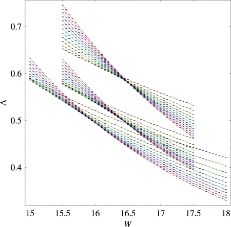
Figure 1: (Color online) $\Lambda(W,L)$ calculated for $t=0,0.25,1$, going from the bottom set of points to the top, with corresponding fits (lines). In each set the fastest changing $\Lambda(W)$ corresponds to the largest $L$ studied. Sets of points for intermediate values of $t$ smoothly interpolate between the values in the Figure and are omitted for clarity.

The calculated values of $\Lambda(W,L)$ for $t=0,0.25$ and $1$ are presented in Fig. 1, together with the lines corresponding to the fits. The Fig. shows an increase of $\Lambda(L)$ with $L$ for smaller values of $W$ and a decrease for larger $W$, which correspond, respectively, to the delocalized (metallic) and localized (insulating) behavior. The same values with the corrections to scaling, Eq. (3), subtracted are shown in Fig. 2, and the critical point is where all curves cross. Figure 3 shows the data collapse, where the upper branch corresponds to the metallic ($w<0$) and the lower branch to the insulating ($w>0$) phase.

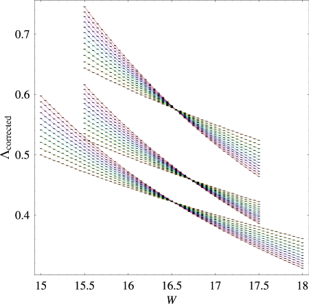
Figure 2: (Color online) Same as in Fig. 1 after the subtraction of the correction to scaling due to the irrelevant field.

Figure 3: Data collapse for $t=0,0.25,0.5,0.7,$ and $1$ (from the bottom two curves to the top).

The obtained values of $\nu,\Lambda_{c},y,$ and $W_{c}$ are presented, respectively, in Fig. 4 and 5. The results in the case of open ($t=0$) and periodic ($t=1$) boundaries for BD are in excellent agreement with Ref. Slevin99 ; Slevin00 . They support the universality of $\nu$, and non-universal, $t$-dependent, $\Lambda_{c}$, $W_{c}$ and $y$. $\Lambda_{c}(t)$ is, however, found to be independent of the distribution of $\epsilon$, which therefore supports the universality of the function $\Lambda_{c}(t)$.

Most remarkably, the results suggest that $W_{c}(t)$ is not constant, i.e, the boundary hopping term $t$ induces a shift of the critical point of the infinite system. To understand this better, we recall that in the classical systems with short-range interaction and the local order-parameter, one generally expects surface ordering with a different critical temperature $T_{c}$ from that in the bulk, but the $T_{c}$ of the bulk is not affected by the presence of boundaries Cardy96 . If these assumptions are generic for any theory with local order-parameter and short-range interactions, and having in mind that disorder plays the analogous role to temperature in classical phase transitions, one arrives to the conclusion that there is no such theory in the universality class of the $H$ studied here for generic values $t_{x,y,z}\neq 0,1$. It should be noted that the non-constant $W_{c}(t)$ found here is not in contradiction with the OPF description of the transition, since OPF at a given point is defined as an integral involving values of $Q$-fields at all other points of the sample.

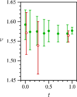
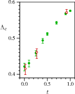
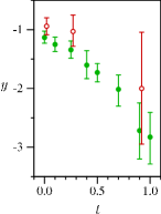
Figure 4: (Color online) Obtained values of the $\nu,\Lambda_{c}$ and $y$ for box (filled circles) and Lorentzian (open circles) distributions of disorder. The latter are slightly displaced along the $x$-axis for clarity. Error bars are $95\%$ confidence intervals.

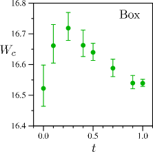
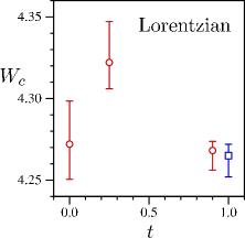
Figure 5: (Color online) Dependence of the critical disorder strength $W_{c}(t)$ (mobility edge) for the box (left panel) and Lorentzian (right panel) distribution of on-site energies, separating the metallic ($W<W_{c}$) from the insulating ($W>W_{c}$) phase. The value $W_{c}(t=1)$ in the Lorentzian case is from Ref. Slevin99 . Error bars are $95\%$ confidence intervals.

In addition to $H$ with constant $t$, systems where each individual boundary hopping term, $t_{ij}$, is an i.i.d random variable were studied for three distributions: $t_{ij}\in[0,1)$, $t_{ij}\in[-1,1)$, and when $t_{ij}$ takes the values 0 or 1 with the probability 1/2. In all three cases BD is used for $\epsilon_{i}$. The results for $\nu,W_{c},\Lambda_{c}$ and $y$ in all three cases give values close to those obtained for $t=0.5$, thus suggesting that randomness in boundary hopping terms can be described by $H$ with an effective constant $t$.

Furthermore, the $t_{x}\neq t_{y}$ case was studied as well for $t_{x}=0.7,t_{y}=0$, when $\Lambda_{c}\approx 0.47(2)$ was obtained for both BD and LD. Since they differ from $\Lambda_{c}(t_{x}=t_{y}=0.7)=0.543_{38}^{47}$, it seems reasonable to expect that there is also a universal $\Lambda_{c}(t_{x},t_{y})$ function independent of the distribution of on-site energies.

Finally, the $t=-0.1$ case with BD of $\epsilon_{i}$ was studied to see effects of the sign of $t$ on critical properties, and results for $\nu,W_{c},\Lambda_{c},$ and $y$ are approx. the same as those obtained for $t=0.1$. This is not surprising since it was already found Slevin00 that the change from periodic to antiperiodic b.c. does not affect critical properties. From these two results it seems reasonable to infer that $\Lambda_{c}(t)\approx\Lambda_{c}(-t)$.

In conclusion, the Anderson model with the boundary hopping term $t$ is studied near the localization-delocalization transition in the presence of the time-reversal symmetry for two distributions of on-site energies. After the careful estimation of statistical errors, the universality of $\nu$ and $\Lambda_{c}(t)$ is shown, and found that $W_{c}$ depends of $t$, which is interpreted as the absence of the local order-parameter description of the transition. The surprising deviation of up to $1\%$ of $W_{c}(t)$ remains to be explained, for example by a theory that would account for the occurrence of the maximum of $W_{c}$ at $t\approx 0.25$.

References

- (1) P. W. Anderson, Phys. Rev. 109, 1492 (1958).
- (2) E. Abrahams, P. W. Anderson, D. C. Licciardello and T. V. Ramakrishnan, Phys. Rev. Lett. 42, 673 (1979).
- (3) B. L. Altshuler, P. A. Lee, and R. A. Webb, eds., Mesoscopic Phenomena in Solids (North-Holland, Amsterdam, 1991).
- (4) B. Shapiro, Phys. Rev. B 34, 4394 (1986); Philos. Mag. B 56, 1031 (1987); B. L. Altshuler, V. E. Kravtsov, and I. V. Lerner, Phys. Lett. A 134, 488 (1989); B. Shapiro, Phys. Rev. Lett. 65, 1510 (1990); K. Slevin, P. Markoš, and T. Ohtsuki, Phys. Rev. Lett. 86, 3594 (2001); Phys. Rev. B 67, 155106 (2003).
- (5) K. B. Efetov, Adv. Phys. 32, 53 (1983).
- (6) S. Hikami, Phys. Rev. B 24, 2671 (1981); V. E. Kravtsov, I. V. Lerner, and V. I. Yudson, Sov. Phys. JETP 67, 1441 (1988). F. Wegner, Nucl. Phys. B 316, 663 (1989); Z. Phys. B: Condens. Matter 78, 33 (1990); E. Breźin and S. Hikami, Phys. Rev. B 55, R10169 (1992); S. Hikami, Prog. Theor. Phys. Suppl. 107, 213 (1992).
- (7) J. L. Pichard and G. Sarma, J. Phys. C 34, L127 (1981).
- (8) A. MacKinnon and B. Kramer, Phys. Rev. Lett. 47, 1546 (1981); Z. Phys. B: Condens. Matter 53, 1 (1983); B. Kramer and A. MacKinnon, Rep. Prog. Phys. 56, 1469 (1993).
- (9) A. MacKinnon, J. Phys.: Condens. Matter 6, 2511 (1994).
- (10) K. Slevin and T. Ohtsuki, Phys. Rev. Lett. 82, 382 (1999).
- (11) B. Bulka, B. Kramer, and A. MacKinnon, Z. Phys. B: Condens. Matter 60, 13 (1985); B. Bulka, M. Schreiber, and B. Kramer, Z. Phys. B: Condens. Matter 66, 21 (1987).
- (12) F. J. Wegner, Z. Phys. B: Condens. Matter 25, 327 (1976).
- (13) M. R. Zirnbauer, Phys. Rev. B 34, 6394 (1986).
- (14) A. D. Mirlin and Y. V. Fyodorov, Phys. Rev. Lett. 72, 526 (1994).
- (15) C. M. Soukoulis, X. Wang, Q. Li, and M. M. Sigalas, Phys. Rev. Lett. 82, 668 (1999); K. Slevin and T. Ohtsuki, Phys. Rev. Lett. 82, 669 (1999).
- (16) D. Braun, E. Hofstetter, G. Montambaux, and A. MacKinnon, Phys. Rev. B 64, 155107 (2001).
- (17) B. I. Shklovskii, B. Shapiro, B. R. Sears, P. Lambrianides, and H. B. Shore, Phys. Rev. B 47, 11487 (1993).
- (18) D. Braun, G. Montambaux, and M. Pascaud, Phys. Rev. Lett. 81, 1062 (1998).
- (19) K. Slevin, T. Ohtsuki, and T. Kawarabayashi, Phys. Rev. Lett. 84, 3915 (2000).
- (20) H. Potempa and L. Schweitzer, J. Phys. Condens. Matter 10, L431 (1998).
- (21) V. E. Kravtsov and V. I. Yudson, Phys. Rev. Lett. 82, 157 (1999).
- (22) S. N. Evangelou, J. Phys. A: Math. Gen. 38 (2005).
- (23) K. Slevin, Y. Asada, and L. I. Deych, Phys. Rev. B 70, 054201 (2004).
- (24) J. Cardy, Scaling and Renormalization in Statistical Physics (Cambridge University Press, Cambridge, 1996).
- (25) B. Huckestein, Phys. Rev. Lett. 72, 1080 (1994).
- (26) Z. Wang, B. Jovanović, and D.-H. Lee, Phys. Rev. Lett. 77, 4426 (1996).
- (27) L. Schweitzer and P. Markoš, Phys. Rev. Lett. 95, 256805 (2005).
- (28) W. H. Press, A. A. Teukolsky, W. T. Vetterling, and B. P. Flannery, Numerical Recipes in C (Cambridge University Press, Cambridge, 1992), 2nd ed.