Theory of conserved spin current and its application to two dimensional hole gas

Abstract

We present a detailed microscopic theory of the conserved spin current which is introduced by us [Phys. Rev. Lett. 96, 196602 (2006)] and satisfies the spin continuity equation even for spin-orbit coupled systems. The spin transport coefficients $\sigma_{\mu\nu}^{s}$ as a response to the electric field are shown to consist of two parts, i.e., the conventional part $\sigma_{\mu\nu}^{s0}$ and the spin torque dipole correction $\sigma_{\mu\nu}^{s\tau}$. As one key result, an Onsager relation between $\sigma_{\mu\nu}^{s}$ and other kinds of transport coefficients are shown. The expression for $\sigma_{\mu\nu}^{s}$ in terms of single-particle Bloch states are derived, by use of which we study the conserved spin Hall conductivity in the two dimensional hole gas modeled by a combined Luttinger and SIA Rashba spin-orbit coupling. It is shown that the two components in spin Hall conductivity usually have the opposite contributions. While in the absence of Rashba spin splitting, the spin Hall transport is dominated by the conventional contribution, the presence of Rashba spin splitting stirs up a large enhancement of the spin torque dipole correction, leading to an overall sign change for the total spin Hall conductivity. Furthermore, an approximate two-band calculation and the subsequent comparison with the exact four-band results are given, which reveals that the coupling between the heavy hole and light hole bands should be taken into account for strong Rashba spin splitting.

I Introduction

Spintronics which combines the basic quantum mechanics of coherent spin dynamics and technological applications in information processing and storage devicesWolf ; Awsch ; Das , has grown up to become a very active and promising field in condensed matter. One central issue in spintronics is on how to generate and manipulate spin current as well as to exploit its various effects in a variety kinds of systems, ranging from ferromagnetic metals to semiconductor paramagnets. In the ideal situation where spin is a good quantum number, spin current is simply defined as the difference between the currents of electron carried by the two spin states. This concept of the spin current has served well in early studies of spin-dependent transport effects in metals. The ubiquitous presence of spin-orbit coupling inevitably makes the spin non-conserved, but this inconvenience is usually put off by focusing one’s attention within the so-called spin relaxation time. In recent years, it has been found that the extrinsic or intrinsic spin-orbit coupling can provide a route to generate transverse spin current in ferromagnetic metalsHirsch ; Zhang or semiconductor paramagnetsDya ; Muk1 ; Sinova by the driving of an electric field. The fundamental question of how to define the spin current properly in the general situation then needs to be answered. In most of previous studies of bulk spin transport, it has been conventional to define the spin current simply as a combined thermodynamic and quantum-mechanical average over the symmetric product of spin and velocity operators. Unfortunately, no viable measurement is known to be possible for this spin current. The recent spin-accumulation experimentsKato ; Wund ; Sih do not directly determine it, and there is no deterministic relation between this spin current and the boundary spin accumulation.

In fact, the conventional definition of spin current suffers critical flaws that prevent it from being relevant to spin transport and accumulation. First, this spin current is not conserved, rendering it useless in describing a true “current”; Second, this spin current does not necessarily vanish in insulatorsFang ; Mura2004 , and in thermodynamic equilibriumRashba2003 , so it is disqualified as a true transport current corresponding to spin accumulation; Finally, there does not exist a mechanical or thermodynamic force in conjugation with this current, so it cannot be fitted into the standard near-equilibrium transport theory. The last issue in particular makes the direct measurement of the conventional spin current difficult if not impossible. For instance, because the conventional spin transport coefficients cannot be associated with other transport coefficients via Onsager relationPZhang , they cannot be measured by linking to other transport phenomena.

These issues were addressed in our last brief reportShi , where we have established a proper definition of spin current free from all the above difficulties. The new spin current is given by the time derivative of the spin displacement (product of spin and position observables), which differs from the conventional definition by a torque dipole term. The torque dipole term is first found in a semiclassical theoryCulcer2004 , whose impact on spin transport has been further analyzed to assess the importance of the inverse spin Hall effectPZhang , i.e., the charge Hall effect driven by a spin force. The new spin transport coefficients $\sigma_{\mu\nu}^{s}$ are shown to consist of two parts, i.e., the conventional part $\sigma_{\mu\nu}^{s0}$ and the spin torque dipole correction $\sigma_{\mu\nu}^{s\tau}$. As one key result, the Onsager relation between $\sigma_{\mu\nu}^{s}$ and other kinds of force-driven transport coefficients has been shown. Note that the other alternative definitions of spin current have also been proposed recentlyJin2005 ; Murakami2004 ; Zhang2005 ; Sun2005 ; Wang2006 .

In this paper, a detailed quantum-mechanical linear response theory of this conserved spin current is addressed, which will be shown itself a necessary supplement as well as an enlightening illustration for our previous brief reportShi . In particular, a general Kubo formula for the spin transport coefficients $\sigma_{\mu\nu}^{s}$ in terms of single-particle Bloch states is given in this paper. Then we use our formula to study the conserved spin Hall conductivity in the two dimensional hole gas (2DHG) modeled by a combined bulk Luttinger and space-inversion asymmetric (SIA) Rashba spin-orbit coupling. It is shown that the two components in spin Hall conductivity usually have the opposite contributions. While in the absence of Rashba spin splitting, the spin Hall transport is dominated by the conventional contribution, the presence of Rashba spin splitting stirs up a large enhancement of the spin torque dipole correction, leading to an overall sign change for the total spin Hall conductivity. Furthermore, an approximate two-band calculation and the subsequent comparison with the exact four-band results are given, which reveals that the coupling between the heavy hole and light hole bands should be taken into account for strong Rashba spin splitting.

Our paper is organized as follows. In Sec. II we give a brief review of the conserved spin current defined in Ref.Shi . The intuitive arguments begin with a search for spin density continuity equation by taking into account the spin torque dipole correction. In Sec. III we clarify the necessity to include the spin torque dipole correction into the total spin current by initiating a linear response analysis. That is, only when this spin torque dipole correction is included, can the proper Onsager relations between the spin transport coefficients and the other transport coefficients be established, which turn out to be essential to endow the spin current a driving force. In Sec. IV we present a Kubo formula for the conserved spin transport coefficients in terms of single-particle eigenstates. In Sec. V we give a detailed discussion of the spin Hall effect in the two dimensional hole gas by use of our general formulae. The analytic and numerical calculation are given both in weak and strong SIA spin-orbit coupling regimes and show very different features concerning the interplay between the two components in the total spin Hall conductivity. Finally, in Sec. VI we present our conclusions.

II Spin continuity equation and introdution of conserved spin current

The conventional definition of the spin current is the expectation value of the product of spin and velocity operators. In the case of spin-polarized magnetic systems, this spin current is simply reduced to the difference between the spin-up and spin-down electrical currents. In the case of spin-orbit stronly coupled semiconductor systems, where time-reversal symmetry ensures no bulk spin polarization, unfortunately, no viable measurement is known to be related with the conventional spin current. This can be straightforwardly shown by writing down the continuity equation for spin density,

$$\frac{\partial S_{z}}{\partial t}+\nabla\cdot\mathbf{J}_{s}=\mathcal{T}_{z}\,.$$ (1)

The spin density for single-particle (spinor) state $\psi(\mathbf{r})$ is defined by $S_{z}(\mathbf{r})=\psi^{\dagger}(\mathbf{r})\hat{s}_{z}\psi(\mathbf{r})$, where $\hat{s}_{z}$ is the spin operator for a particular component ($z$ here, to be specific). The spin current density is given by the conventional definition $\mathbf{J}_{s}(\mathbf{r})=\operatorname{Re}\psi^{\dagger}(\mathbf{r})\frac{1}{2}\{\hat{\mathbf{v}},\,\hat{s}_{z}\}\psi(\mathbf{r})$, where $\hat{\mathbf{v}}$ is the velocity operator, and $\{,\}$ denotes the anticommutator. The right hand side of the Eq. (1) is the spin torque density defined by $\mathcal{T}_{z}(\mathbf{r})=\operatorname{Re}\psi^{\dagger}(\mathbf{r})\hat{\tau}\psi(\mathbf{r})$, where $\hat{\tau}\equiv d\hat{s}_{z}/dt\equiv(1/i\hbar)[\hat{s}_{z},\,\hat{H}]$, and $\hat{H}$ is the Hamiltonian of the system. The presence of the torque density $\mathcal{T}_{z}$ reflects the fact that spin is not conserved microscopically in systems with spin-orbit coupling. As a consequence, the only knowledge about the experimentally measured variation of spin density in space-time is not sufficient to determine the conventional spin current $\mathbf{J}_{s}$, and vice versa, due to the unique presence of the spin torque density $\mathcal{T}_{z}$ in spin-orbit coupled systems.

One promising choiceShi to remedy this oblique relationship between spin density and spin current is to formaly move the torque density term to the left hand side of Eq. (1) and absorb it in the divergence term. The physical reason is that, due to symmetry reasons, it often happens that the average torque vanishes for the bulk of the system, i.e., $(1/V)\int dV\mathcal{T}_{z}(\mathbf{r})=0$. Thus one can write the torque density as a divergence of a torque dipole density,

$$\mathcal{T}_{z}(\mathbf{r})=-\nabla\cdot\mathbf{P}_{\tau}(\mathbf{r})\,.$$ (2)

Moving it to the left hand side of Eq. (1), one has

$$\frac{\partial S_{z}}{\partial t}+\nabla\cdot\left(\mathbf{J}_{s}+\mathbf{P}_{\tau}\right)=0\,,$$ (3)

which is in the form of the standard sourceless continuity equation. This shows that the spin is conserved on average in such systems, and the corresponding transport spin current is:

$$\boldsymbol{\mathcal{J}}_{s}=\mathbf{J}_{s}+\mathbf{P}_{\tau}.$$ (4)

Note that there is still an arbitrariness in defining the effective spin current because Eq. (2) does not uniquely determine the torque dipole density $\mathbf{P}_{\tau}$ from the corresponding torque density $\mathcal{T}_{z}$. However, this ambiguity can be eliminated by imposing the physical constraint that the torque dipole density is a material property that should vanish outside the sample. This implies in particular that $\int dV\,\mathbf{P}_{\tau}=-\int dV\,\mathbf{r}\nabla\cdot\mathbf{P}_{\tau}=\int dV\,\mathbf{r}\mathcal{T}_{z}(\mathbf{r})$. It then follows that, upon bulk average, the effective spin current density can be written as $\boldsymbol{\mathcal{J}}_{s}=\operatorname{Re}\psi^{\ast}(\mathbf{r})\hat{\boldsymbol{\mathcal{J}}}_{s}\psi(\mathbf{r})$, where

$$\hat{\boldsymbol{\mathcal{J}}}_{s}=\frac{\mathrm{d}(\hat{\mathbf{r}}\hat{s}_{z})}{\mathrm{d}t}\,$$ (5)

is the effective spin current operator. Compared to the conventional spin current operator, it has an extra term $\hat{\mathbf{r}}(\mathrm{d}\hat{s}_{z}/\mathrm{d}t)$, which accounts the contribution from the spin torque.

The conservation of the new spin current allows one to consider spin transport in the bulk without the need of laboring explicitly a spin torque (dipole density) which may be generated by the electric field. Thus the spin transport in spin-orbit coupled systems can be treated in a unified way, whatever the spin-orbit coupling strength is weak or strong. For example, it has been customary to link spin density and spin current through the following phenomenological spin continuity equation,

$$\frac{\partial S_{z}}{\partial t}+\nabla\cdot\boldsymbol{\mathcal{J}}_{s}=-\frac{S_{z}}{\tau_{s}},$$ (6)

where $\tau_{s}$ is the spin relaxation time, and the spin current has the form $\boldsymbol{\mathcal{J}}_{s}=\sigma E-D_{s}\nabla S_{z}$. This makes sense only if our new spin current is used in the calculation of spin conductivity $\sigma$, otherwise an extra term of field-generated spin torque must be added.

Equation (6) now can serve as the basis to determine the spin accumulation at a sample boundary. Consider a system having a smooth boundary produced by a slowly varying confining potential. We assume that the length scale of variation is much larger than the mean free path, so that the above continuity equation may be applied locally. By integrating from the interior to the outside of the sample boundary, we obtain a spin accumulation per area with $S_{z}=\boldsymbol{\mathcal{J}}_{s}^{\text{bulk}}\tau_{s}$. Thus one can see that for the generic class of smooth boundaries, there is a unique relationship between spin accumulation and the conserved spin current $\boldsymbol{\mathcal{J}}_{s}$, instead of the conventional spin current $\mathbf{J}_{s}$. The other kinds of boundary conditions have also been discussed in previous workShi ; Nomura ; Tse to clarify the relationship beween spin accumulation and bulk spin current.

III Spin Hall conductivity and its Onsager relation with inverse spin Hall effect

Defined as a time derivative of the spin displacement operatore $\hat{\mathbf{r}}\hat{s}_{z}$, the new spin current has a natural conjugate force, i.e., the spin force, $\mathbf{F}_{s}$. To show this, one can consider the system exposed to an inhomogeneous Zeeman magnetic field along $z$-axis. The resulting perturbation can be modeled as $V(\mathbf{r})=g^{\ast}\mu_{B}B(\mathbf{r})\hat{s}_{z}$ with Bohr magneton $\mu_{B}$ and effective magnetic factor $g^{\ast}$. Suppose that the inhomogeneous Zeeman field is smoothly varying in space around zero. Then the first-order expansion in position operator givesZutic2002 ; PZhang

$$V=-\mathbf{F}_{s}\cdot(\hat{\mathbf{r}}\hat{s}_{z})$$ (7)

with a spin force $\mathbf{F}_{s}=-\nabla(g^{\ast}\mu_{B}B(\mathbf{r}))$ applying on the carriers. Thus it becomes clear now that only when the spin current is defined as a time derivative of the spin displacement operator $\hat{\mathbf{r}}\hat{s}_{z}$, can there naturally arises a conjugate driving force $\mathbf{F}_{s}$. As a consequence, the energy dissipation rate for the spin transport can be written as $\mathrm{d}Q/\mathrm{d}t=\boldsymbol{\mathcal{J}}_{s}{\small\cdot}\mathbf{F}_{s}$. It immediately suggests a thermodynamic way to determine the spin current by simultaneously measuring the Zeeman field gradient (spin force) and the heat generation.

The existence of a physical driving force for the conserved spin current makes it possible to construct Onsager relation between spin transport coefficients and other kinds of force-driving transport coefficients. For instance, since an electric force $\mathbf{E}$ may drive a spin-Hall current through the spin-orbit interaction, one naturally expects that a spin force $\mathbf{F}_{s}$ may also induce a charge-Hall current. Naturally, an exact Onsager relation between these intrinsic Hall effects may be established: In a general sense, when two kinds of different forces, say a spin force $\mathbf{F}_{s}$ and an electric force $\mathbf{E}$ coexist as driving forces, then the linear charge-current and spin-current responses to these two forces can be expressed as

$$\left(\begin{array}[c]{c}\boldsymbol{\mathcal{J}}_{s}\\ \mathbf{J}_{c}\end{array}\right)=\left(\begin{array}[c]{cc}\overleftrightarrow{\sigma}^{ss}&\overleftrightarrow{\sigma}^{sc}\\ \overleftrightarrow{\sigma}^{cs}&\overleftrightarrow{\sigma}^{cc}\end{array}\right)\left(\begin{array}[c]{c}\mathbf{F}_{s}\\ \mathbf{E}\end{array}\right),$$ (8)

where $\boldsymbol{\mathcal{J}}_{s}$ is spin current and $\mathbf{J}_{c}$ charge current. $\overleftrightarrow{\sigma}^{ss}$ ($\overleftrightarrow{\sigma}^{cc}$) is the spin-spin (charge-charge) $3\times 3$ conductivity tensor characterizing spin (charge) current response to a spin (charge) force $\mathbf{F}_{s}$ ($\mathbf{E}$). In the same manner, the off diagonal block $\overleftrightarrow{\sigma}^{sc}$ denotes spin current response to an electric field, and $\overleftrightarrow{\sigma}^{cs}$ denotes charge current response to a spin forcePZhang . A general relationship between $\overleftrightarrow{\sigma}^{sc}$ and $\overleftrightarrow{\sigma}^{cs}$ can be explicitly derived with a proper definition of the spin current, or imposed by the general Onsager relationCasimir :

$$\sigma_{\alpha\beta}^{sc}=\varepsilon_{\alpha}\varepsilon_{\beta}\sigma_{\beta\alpha}^{cs}$$ (9)

where $\varepsilon_{\alpha}$, $\varepsilon_{\beta}$ are equal to $+1$ or $-1$ depending on whether the displacement (corresponding to current) operator is even or odd under time reversal operation $T$. In the present case, the displacement for a spin force is odd under $T$, while the displacement for an electric field is $T$-invariant, implying $\varepsilon_{\alpha}\varepsilon_{\beta}=-1$.

Here the key point is that the Onsager relation is only attainable when the spin current is corrected by a torque dipole term. To see this more clearly, we employ a standard Kubo formula description as follows: Let us put a spin force along $\mu$-direction and an electric field $E$ along $\nu$-direction on equal footing by including both of them in the total Hamiltonian, $H=H_{0}-F_{1}d_{1}-F_{2}d_{2}$, where $F_{1}=E$ and $F_{2}=F^{s}$ are the generalized forces applied on the charge and spin degrees of freedom, whereas $d_{1}=-ex_{\mu}$ and $d_{2}=s_{z}x_{\nu}$ are the corresponding displacement operators in which $x_{\mu}$ denotes the $\mu$-component of the position observable $\mathbf{r}$. The response currents are obtained as the expectation values of the generalized velocity operators in the perturbed states,

$$\dot{d}_{1}=-e\dot{x}_{\mu},\text{ }\dot{d}_{2}=s_{z}\dot{x}_{\nu}+\dot{s}_{z}x_{\nu}\mathbf{,}$$ (10)

where the standard symmetrization procedure in $\dot{d}_{2}$ is implied. The presence of these two external forces will change an arbitrary stationary quantum state $|\alpha\rangle$ of the original Hamiltonian into $|\alpha^{\prime}\rangle=|\alpha\rangle+\sum_{\beta\neq\alpha,i=1,2}|\beta\rangle\langle\beta|F_{i}d_{i}|\alpha\rangle/(\epsilon_{\alpha}-\epsilon_{\beta}+i\eta)$, where $\epsilon_{\alpha}$ is unperturbed energy for $|\alpha\rangle$ and $\eta\rightarrow 0$ arises from the fact that when time $t\rightarrow-\infty$, the perturbation is adiabatically switched off. Then the currents as a linear response to the perturbations are, after a straightforward derivation and by noting the substitution $\langle\beta|d_{i}|\alpha\rangle=\frac{i\hbar}{\varepsilon_{\alpha}-\varepsilon_{\beta}}\langle\beta|\dot{d}_{i}|\alpha\rangle$, given by $\langle\dot{d}_{i}\rangle=\sum_{\alpha^{\prime}}f_{\alpha^{\prime}}\langle\alpha^{\prime}|\dot{d}_{i}|\alpha^{\prime}\rangle\equiv\sum_{j}\sigma_{ij}F_{j}$ with the conductivity matrix

$$\sigma_{ij} =\sum_{\alpha\neq\beta}\frac{\hbar\operatorname{Im}[\langle\alpha|\dot{d}_{i}|\beta\rangle\langle\beta|\dot{d}_{j}|\alpha\rangle]}{(\epsilon_{\alpha}-\epsilon_{\beta})^{2}+\eta^{2}}(f_{\alpha}-f_{\beta})$$ (11)

$$+\sum_{\alpha\neq\beta}\frac{df_{\alpha}(\epsilon)}{d\epsilon}\operatorname{Re}[\langle\alpha|\dot{d}_{i}|\beta\rangle\langle\beta|\dot{d}_{j}|\alpha\rangle]\delta(\epsilon_{\alpha}-\epsilon_{\beta})$$

Here $f_{\alpha}$ is the equilibrium fermi function for band $\epsilon_{\alpha}$. Obviously, the first term is antisymmetric under the inter-exchange $i\leftrightarrow j$, while the second term is the symmetric part of $\sigma_{ij}$. While the symmetric part denotes dissipative contribution to the charge or spin transport, the first antisymmetric term is dissipationless and is relevant to our discussion in this paper. For an ideal system without scattering and many-body interaction, it is obvious that the dissipative (symmetric) part in Eq.(11) vanishes. The dissipationless conductivity has manifested itself in a fundamental way in condensed matter physics involving such issues as quantum and anomalous Hall effects. Our present discussions, as well as recent active studies of spin-Hall effect, are also focused on this dissipationless part of the transport conductivity.

It becomes clear from Eqs.(10)-(11) that the intrinsic spin-Hall conductivity is given by

$$\sigma_{\mu\nu}^{s}=-e\sum_{\alpha\neq\beta}\frac{\hbar\operatorname{Im}[\langle\alpha|s_{z}\dot{x}_{\mu}+\dot{s}_{z}x_{\mu}|\beta\rangle\langle\beta|\dot{x}_{\nu}|\alpha\rangle]}{(\varepsilon_{\alpha}-\varepsilon_{\beta})^{2}+\eta^{2}}(f_{\alpha}-f_{\beta}),$$ (12)

where again symmetrization is implied in the product of two operators. On the other side, the dissipationless inverse spin-Hall conductivity driven by a spin force is given by

$$\sigma_{\nu\mu}^{c}=-e\sum_{\alpha\neq\beta}\frac{\hbar\operatorname{Im}[\langle\alpha|\dot{x}_{\nu}|\beta\rangle\langle\beta|s_{z}\dot{x}_{\mu}+\dot{s}_{z}x_{\mu}|\alpha\rangle]}{(\varepsilon_{\alpha}-\varepsilon_{\beta})^{2}+\eta^{2}}(f_{\alpha}-f_{\beta})$$ (13)

The antisymmetric property shown above immediately gives the equality

$$\sigma_{\mu\nu}^{s}=-\sigma_{\nu\mu}^{c}$$ (14)

which coincides with the general Onsager relation (9). Note that Eq.(14) denotes the Onsager relation only for the dissipationless (antisymmetric) part in conductivities. A full Onsager relation by taking into account impurity scattering and an external uniform magnetic field $B_{0}$ turns out to be given by $\sigma_{\mu\nu}^{s}(B_{0},\tau_{0})=-\sigma_{\nu\mu}^{c}(-B_{0},-\tau_{0})$, where $\tau_{0}$ characterizes scattering-induced relaxation time. Therefore, from Eqs.(12)-(13) one can see that to ensure the Onsager relation between the two kinds of Hall conductivities, the spin current should be defined as

$$\boldsymbol{\mathcal{J}}_{s}=\frac{\mathrm{d}(\hat{\mathbf{r}}\hat{s}_{z})}{\mathrm{d}t}$$ (15)

instead of conventional definition.

The above arguments clearly show two prominent features of the new spin current which is absent within the conventional definition of the spin current: (i) The spin current is now conserved with a physical conjugate driving force; (ii) The Onsager relation is built up. Besides these two prominent featues, there is another physically valid property: For simple insulators whose single particle eigenstates are localized (Anderson insulators), the spin transport coefficients vanish. Indeed, for spatially localized eigenstates, we can evaluate the (intrinsic) conductivity from Eq. (12) as,

$$\sigma^{s} =-e\hbar\sum_{\alpha\neq\beta}f_{\alpha}\frac{\operatorname{Im}[\langle\alpha|\mathrm{d}(\hat{\mathbf{r}}\hat{s}_{z})/\mathrm{d}t|\beta\rangle\langle\beta|\mathbf{\hat{v}}|\alpha\rangle]}{(\epsilon_{\alpha}-\epsilon_{\beta})^{2}}$$ (16)

$$=-e\hbar\sum_{\alpha}f_{\alpha}\langle\alpha|[\hat{\mathbf{r}}\hat{s}_{z},\hat{\mathbf{r}}]|\alpha\rangle=0$$

where we have used $\langle\alpha|\mathrm{d}(\hat{\mathbf{r}}\hat{s}_{z})/\mathrm{d}t|\beta\rangle=\frac{i}{\hbar}(\epsilon_{\alpha}-\epsilon_{\beta})\langle\alpha|\hat{\mathbf{r}}\hat{s}_{z}|\beta\rangle$ and $\langle\beta|\mathbf{\hat{v}}|\alpha\rangle=\frac{i}{\hbar}(\epsilon_{\beta}-\epsilon_{\alpha})\langle\beta|\hat{\mathbf{r}}|\alpha\rangle$. The involved matrix elements are well defined between spatially localized eigenstates.

IV Kubo formula for conserved spin transport coefficients

In this section we show how to evaluate in practice the conserved spin Hall conductivity based on the new definition of spin current in a crystal. A formal description has been given in Eq. (10) for the conserved spin conductivity, while the general states $|\alpha\rangle$ should now be replaced by the electron Bloch wave function $\psi_{nk}(\mathbf{r})$. Clearly, the conserved spin Hall conductivity includes two components,

$$\sigma_{\mu\nu}^{s}=\sigma_{\mu\nu}^{s0}+\sigma_{\mu\nu}^{s\tau}.$$ (17)

The first one is the usual conventional spin Hall coefficient, which is ready to be rewritten in the Bloch-state space as

$$\sigma_{\mu\nu}^{s0} =-e\hbar\sum_{n\neq n^{\prime},\mathbf{k}}\left[f(\epsilon_{n\mathbf{k}})-f(\epsilon_{n^{\prime}\mathbf{k}})\right]\times$$ (18)

$$\frac{\operatorname{Im}\langle u_{n\mathbf{k}}|\frac{1}{2}\{\hat{v}_{\mu},\hat{s}_{z}\}|u_{n^{\prime}\mathbf{k}}\rangle\langle u_{n^{\prime}\mathbf{k}}|\hat{v}_{\nu}|u_{n\mathbf{k}}\rangle}{\left(\epsilon_{n\mathbf{k}}-\epsilon_{n^{\prime}\mathbf{k}}\right)^{2}+\eta^{2}}.$$

Here $\mathbf{\hat{v}}(\mathbf{k})=\partial H(\mathbf{k})/\hbar\partial\mathbf{k}$, $H(\mathbf{k})=\exp(-i\mathbf{k}{\small\cdot}\mathbf{r})\hat{H}\exp(i\mathbf{k}{\small\cdot}\mathbf{r})$, $|u_{n\mathbf{k}}\rangle$ is the periodic part of the electron carrier Bloch wave function, and ($-e$) is the electron charge. The Kubo formula (18) for the conventional spin Hall conductivity has been used by most of previous investigationsSinova .

The second component $\sigma_{\mu\nu}^{s\tau}$ in the conserved spin-Hall conductivity, as shown in Eq. (4) and Eq. (12), comes from the contribution of the spin torque density term. Due to the presence of the position operator in this term, and the fact that the position operator is not well-defined in the Bloch-state space, one needs to take some care in dealing with $\sigma_{\mu\nu}^{s\tau}$. As one choice for derivation, we proceed by a regularization scheme, $\dot{s}_{z}x_{\mu}\rightarrow\dot{s}_{z}\sin(q_{\mu}x_{\mu})/q_{\mu}$, followed by the limit $q_{\mu}\rightarrow 0$. The symmetrized $\mu$-component of the spin torque density operator occurred in Eq. (12) can now be rewritten as

$$P_{\tau}=\frac{1}{2}\{\dot{s}_{z},\frac{\sin(qx_{\mu})}{q}\}=\lim_{q\rightarrow 0}\frac{1}{4iq}\left[\{\dot{s}_{z},e^{iqx_{\mu}}\}-\{\dot{s}_{z},e^{-iqx_{\mu}}\}\right]$$ (19)

Substituting Eq. (19) into Eq. (12) and after a straightforward manipulation, we obtain the Kubo formula for $\sigma_{\mu\nu}^{s\tau}$:

$$\sigma_{\mu\nu}^{s\tau} =-e\hbar\lim_{\mathbf{q}\rightarrow 0}\frac{1}{q_{\nu}}\sum_{n\neq n^{\prime},\mathbf{k}}\left[f(\epsilon_{n\mathbf{k}})-f(\epsilon_{n^{\prime}\mathbf{k+q}})\right]\times$$ (20)

$$\frac{\operatorname{Re}[\langle u_{n\mathbf{k}}|\hat{\tau}(\mathbf{k},\mathbf{q})|u_{n^{\prime}\mathbf{k}+\mathbf{q}}\rangle\langle u_{n^{\prime}\mathbf{k}+\mathbf{q}}|\mathbf{\hat{v}}(\mathbf{k},\mathbf{q})|u_{n\mathbf{k}}\rangle]}{\left(\epsilon_{n\mathbf{k}}-\epsilon_{n^{\prime}\mathbf{k+q}}\right)^{2}+\eta^{2}},$$

where $\hat{\tau}(\mathbf{k},\mathbf{q})=\frac{1}{2}\left[\hat{\tau}(\mathbf{k})+\hat{\tau}(\mathbf{k}+\mathbf{q})\right]$ with $\hat{\tau}(\mathbf{k})=(1/i\hbar)[\hat{s}_{z},H(\mathbf{k})]$, $\mathbf{\hat{v}}(\mathbf{k},\mathbf{q})=\frac{1}{2}[\mathbf{\hat{v}}(\mathbf{k})+\mathbf{\hat{v}}(\mathbf{k}+\mathbf{q})]$. The limit of $\eta\rightarrow 0$ should be taken at the last step of calculation, and as a result, there is no intra-band ($n=n^{\prime}$) contribution. Note that to properly calculate $\sigma_{\mu\nu}^{s\tau}$ in practice, all the terms in Eq. (4) with the subscript $\mathbf{k}+\mathbf{q}$ should be expaned at $\mathbf{k}$ to first order in $\mathbf{q}$.

Equation (20) can also be derived from an analysis of the spin torque dipole density $\mathcal{T}_{z}(\mathbf{r})$ which can be determined unambiguously as a bulk property within the theoretical framework of linear response. Consider the torque response to an electric field at finite wave vector $\mathbf{q}$, $\mathcal{T}_{z}(\mathbf{q})=\mathbf{\chi}(\mathbf{q}){\small\cdot}\mathbf{E(q)}$. Based on Eq. (2) which implies $\mathcal{T}_{z}(\mathbf{q})=-i\mathbf{q}{\small\cdot}\mathbf{P}_{\tau}\mathbf{(q)}$, we can uniquely determine the static response (i.e., $\mathbf{q}\rightarrow 0$) of the spin torque dipole:

$$\mathbf{P}_{\tau}\mathbf{(q)=\operatorname{Re}}\{i\nabla_{\mathbf{q}}[\mathbf{\chi}(\mathbf{q}){\small\cdot}\mathbf{E}]\}_{\mathbf{q}=0}.$$ (21)

Here we have utilized the condition $\mathbf{\chi}(0)=0$, i.e., there is no bulk spin generation by the electric field. Thus the consequent spin-transport coefficient for the electric response of the spin torque density is given by

$$\sigma_{\mu\nu}^{s\tau}=\operatorname{Re}[i\partial_{q_{\mu}}\chi_{\nu}(\mathbf{q})]_{\mathbf{q}=0}.$$ (22)

Again within the standard Kubo-formula formalism, the spin torque response coefficient $\mathbf{\chi}(\mathbf{q})$ can be calculated to be

$$\mathbf{\chi}(\mathbf{q}) =ie\hbar\sum_{n\neq n^{\prime},\mathbf{k}}\left[f(\epsilon_{n\mathbf{k}})-f(\epsilon_{n^{\prime}\mathbf{k+q}})\right]\times$$ (23)

$$\frac{\operatorname{Re}[\langle u_{n\mathbf{k}}|\hat{\tau}(\mathbf{k},\mathbf{q})|u_{n^{\prime}\mathbf{k}+\mathbf{q}}\rangle\langle u_{n^{\prime}\mathbf{k}+\mathbf{q}}|\mathbf{\hat{v}}(\mathbf{k},\mathbf{q})|u_{n\mathbf{k}}\rangle]}{\left(\epsilon_{n\mathbf{k}}-\epsilon_{n^{\prime}\mathbf{k+q}}\right)^{2}+\eta^{2}},$$

which, combining Eq. (22), gives the same expression for $\sigma_{\mu\nu}^{s\tau}$ as that in Eq. (20).

Due to the inclusion of contribution from the spin torque dipole term, one may expect that in some special cases the transport properties of the conserved spin current are essentially different from that of conventional spin current. This will turn to be true by studying in the next section the intrinsic spin Hall conductivity in a 2DHG system, which is modeled by a combined Luttinger and spin-3/2 SIA Rashba spin-orbit interactions. For disordered systems, the spin-Hall conductivity based on our new spin current has also been calculated in a recent workSugimoto , and is found to depend explicitly on the scattering potentials for the two dimensional Rashba models with $k$-linear or $k$-cubic spin-orbit coupling. For one who instead prefers the conventional definition of the spin current, the above discussions are of course still helpful due to the fact that one cannot at last avoid tackling the calculation of the spin torque contribution to the total transport spin current and the spin accumulation, while our above derivation clearly indicates how to do that in practice.

V Application to 2DHG system

As a practical application of the above general theory of the conserved spin current to the real physical systems, in this section we focus our attention to the intrinsic spin Hall effect in a 2DHG system, which has been experimentallyWund and theoreticallyBern investigated within the conventional spin-transport framework. Following Ref.Bern , the spin-orbit interaction in this system is modeled by combined Luttinger and spin-3/2 SIA Rashba terms. The resultant $\mathbf{k}{\small\cdot}\mathbf{p}$ Hamiltonian reads ($\hbar$ is set to be unity):

$$H_{0}=(\gamma_{1}+\frac{5}{2}\gamma_{2})\frac{k^{2}}{2m}-\frac{\gamma_{2}}{m}(\mathbf{k{\small\cdot}S})^{2}+\alpha(\mathbf{S}\times\mathbf{k}){\small\cdot}\hat{z},$$ (24)

where the confinement of the quantum well in the $\hat{z}$ direction makes the momentum be quantized on this axis. The crucial difference between SIA Rashba term in 2DHG and SIA Rashba term in the 2DEG lies in the fact that $S$ in 2DHG is spin-3/2 matrix, describing both the heavy (HH) and light (LH) holes. For the first heavy and light hole bands, the confinement in a quantum well of thickness $a$ is approximated by the relation $\langle k_{z}\rangle=0$, $\langle k_{z}^{2}\rangle\approx(\pi/a)^{2}$. The energies for HH and LH are given by

$$E_{\pm}^{LH} =\frac{\gamma_{1}}{2m}(k^{2}+\langle k_{z}^{2}\rangle)\pm\frac{1}{2}\alpha k-\sqrt{\alpha^{2}k^{2}\pm\frac{\alpha\gamma_{2}}{m}k(k^{2}+\langle k_{z}^{2}\rangle)+\frac{\gamma_{2}^{2}}{m^{2}}d^{2}},$$ (25)

$$E_{\pm}^{HH} =\frac{\gamma_{1}}{2m}(k^{2}+\langle k_{z}^{2}\rangle)\pm\frac{1}{2}\alpha k+\sqrt{\alpha^{2}k^{2}\pm\frac{\alpha\gamma_{2}}{m}k(k^{2}+\langle k_{z}^{2}\rangle)+\frac{\gamma_{2}^{2}}{m^{2}}d^{2}},$$

where and in the following $k^{2}=k_{x}^{2}+k_{y}^{2}$, $d=\sqrt{k^{4}+\langle k_{z}^{2}\rangle^{2}-k^{2}\langle k_{z}^{2}\rangle}$. The HH and LH bands are split at the $\Gamma$ point by $\Delta=2\gamma_{2}\langle k_{z}^{2}\rangle/m$. Depending on the confinement scale $a$ the Luttinger term is dominant for $a$ not too small, while the SIA term becomes dominant for thin quantum wells.

By expanding the above formulas for small $k<<\langle k_{z}\rangle$ it is seen that the spin splitting of the HH bands is $k^{3}$ whereas the spin splitting of the LH bands is $k$Bern ,

$$E_{+}^{HH}-E_{-}^{HH} =\frac{3}{8}\frac{\alpha(\alpha^{2}-4\frac{\gamma_{2}^{2}}{m^{2}}\langle k_{z}^{2}\rangle)}{\frac{\gamma_{2}^{2}}{m^{2}}\langle k_{z}^{2}\rangle^{2}}k^{3}+\mathcal{O}(k^{5})$$ (26)

$$E_{+}^{LH}-E_{-}^{LH} =2\alpha k+\mathcal{O}(k^{3})$$

which is in agreement withWink1 ; Wink2 . Figure 1(a) gives a typical band structure for GaAs ($\gamma_{1}=6.92$, $\gamma_{2}=2.1$) with a $\Gamma$ point gap of $40$ meV and a Fermi momentum splitting of the hole band at Fermu momentum ($0.2$ nm^-1) of 5 meV, which requires a SIA splitting $\alpha\approx 50$ meV${\small\cdot}$nm. In the recent experiment of spin-Hall effectWund , this energy gap is of order $\triangle E=40$meV, which corresponds to an $a=8.3$ nm thick quantum well.

Figure 1: (a) Approximate band structure of the GaAs 2DHG; (b) heavy-hole fermi wave vectors as a function Rashba coefficient $\alpha$ for $n_{h}=1.5\times 10^{12}$ cm^-2.

During the following numerical calculation, these three material parameters ($\gamma_{1}$, $\gamma_{2}$, and $a$) will be fixed to be the values mentioned above, whereas the Rashba coefficient $\alpha$ and the hole density $n_{h}$ are treated as the tuning parameters.

First we consider the simple case of thin quantum wells. In this case the SIA Rashba term can be neglected ($\alpha=0$) and a full analytic calculation an be carried out. In the absence of SIA term, the (normalized) eigenstates for HH and LH bands are given by $u_{+}^{HH}=a_{1}|\frac{3}{2},\frac{3}{2}\rangle+a_{2}k_{+}^{2}|\frac{3}{2},-\frac{1}{2}\rangle$, $u_{-}^{HH}=a_{1}|\frac{3}{2},-\frac{3}{2}\rangle+a_{2}k_{-}^{2}|\frac{3}{2},\frac{1}{2}\rangle$, $u_{+}^{LH}=a_{1}|\frac{3}{2},\frac{1}{2}\rangle-a_{2}k_{+}^{2}|\frac{3}{2},-\frac{3}{2}\rangle$, and $u_{-}^{LH}=a_{1}|\frac{3}{2},-\frac{1}{2}\rangle-a_{2}k_{-}^{2}|\frac{3}{2},\frac{3}{2}\rangle$, where $|\frac{3}{2},m_{z}\rangle$ ($m_{z}=\frac{3}{2}$,…$-\frac{3}{2}$) are the eigenstates of $S_{z}$, $k_{\pm}=k_{x}\pm ik_{y}$, $a_{1}=\sqrt{(d-\frac{1}{2}k^{2}+\langle k_{z}^{2}\rangle)/2d}$, $a_{2}=\sqrt{3/8d(d-\frac{1}{2}k^{2}+\langle k_{z}^{2}\rangle)}$. Then using the standard Kubo formula (19) for the conventional spin Hall conductivity, it is straightforward to obtain $\sigma_{xy}^{s0}$ as follows

$$\sigma_{yx}^{0}=-\frac{e}{4\pi}\int(f_{HH}-f_{LH})\left[\frac{3k^{2}}{d^{2}}(a_{1}^{4}-a_{2}^{4}k^{8})+\frac{2\sqrt{3}k^{2}}{\gamma_{2}d^{2}}a_{1}a_{2}k^{2}(a_{1}^{2}+a_{2}^{2}k^{4})(\gamma_{1}+\gamma_{2})\right]kdk.$$

where $f_{HH}$ and $f_{LH}$ are fermi functions for HH and LH respectivel. The spin Hall conductivity due to the contribution from the torque dipole term turns out to be

$$\sigma_{yx}^{s\tau} =\frac{e}{4\pi}\frac{\gamma_{1}}{\gamma_{2}}\int(f_{HH}-f_{LH})\left[\frac{2\sqrt{3}a_{1}a_{2}k^{4}}{d^{2}}(a_{1}^{2}+a_{2}^{2}k^{4})+\frac{3k^{4}}{d^{3}}(a_{1}^{2}+a_{2}^{2}k^{4})^{2}\right]kdk$$ (28)

$$+\frac{e}{4\pi}\int\frac{3k^{4}(a_{1}^{2}+a_{2}^{2}k^{4})^{2}}{2d^{2}}\left(\frac{df_{HH}}{dk}+\frac{df_{LH}}{dk}\right)dk$$

The first line in Eq. (28) is obtained by expanding $|u_{n^{\prime}\mathbf{k}+\mathbf{q}}\rangle$, $\hat{\tau}(\mathbf{k},\mathbf{q})$, and $\epsilon_{n^{\prime}\mathbf{k}+\mathbf{q}}$ in Eq. (20) at $\mathbf{k}$ to the first order in $\mathbf{q}$ while remaining other quantities to be their values at $\mathbf{q}=0$. Whereas the second line in Eq. (28) with $df/dk$ is obtained by a linear expansion of the fermi function with respect to $\mathbf{q}$. The other terms occurring in Eq. (20) turn out to take no contribution to $\sigma_{yx}^{s\tau}$ for the present model. In the strong confinement limit ($k^{2}<\langle k_{z}^{2}\rangle$) and at zero temperature, Eqs. (V)-(28) are reduced to

$$\sigma_{yx}^{s0} =-\frac{e}{4\pi}\left[\frac{3(k_{HH}^{4}-k_{LH}^{4})}{4\langle k_{z}^{2}\rangle^{2}}+\frac{(\gamma_{1}+\gamma_{2})(k_{HH}^{6}-k_{LH}^{6})}{4\gamma_{2}\langle k_{z}^{2}\rangle^{3}}\right],$$

$$\sigma_{yx}^{s\tau} =\frac{e}{4\pi}\left[\frac{3\gamma_{1}(k_{HH}^{6}-k_{LH}^{6})}{4\gamma_{2}\langle k_{z}^{2}\rangle^{3}}-\frac{3(k_{HH}^{4}+k_{LH}^{4})}{2\langle k_{z}^{2}\rangle^{2}}\right].$$ (29)

where $k_{HH}$ and $k_{LH}$ are the fermi wavevectors for HH and LH respectively.

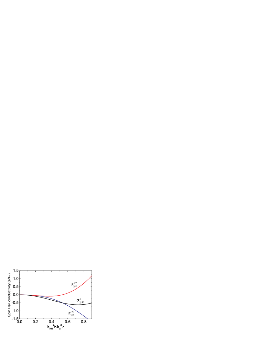
Figure 2: (Color online) conserved spin Hall conductivity $\sigma_{yx}^{s}$ (black line), and its two components $\sigma_{yx}^{s0}$ (blue line) and $\sigma_{yx}^{s\tau}$ (red line) as a function of the heavy hole fermi wave vector for $\alpha=0$ and $n_{h}=1.5\times 10^{12}$ cm^-2.

Since for the experiment data, the LH bands are unoccupied (by the holes), so during numerical calculations throughout this paper we have set the fermi wavevector of the light holes to be zero, $k_{LH}=0$. Based on Eqs. (V)-(28), figure 2 shows the conserved spin Hall conductivity $\sigma_{yx}^{s}$ (black curve) as a function of the fermi wavevector $k_{HH}$ (scaled by the confinement wave vector $\sqrt{\langle k_{z}^{2}\rangle}$) of the heavy holes. For clarification, we have also plotted in Fig. 2 the separate contributions from the conventional part $\sigma_{yx}^{s0}$ (blue curve) and spin torque dipole part $\sigma_{yx}^{s\tau}$ (red cuve); their sum gives $\sigma_{yx}^{s}$. With increasing the fermi wavevector $k_{HH}$, one can see from Fig. 2 that the two components $\sigma_{yx}^{s0}$ and $\sigma_{yx}^{s\tau}$ increase in amplitude but always differ in a sign. The resultant total spin Hall conductivity $\sigma_{yx}^{s}$ displays a non-monotonic behavior. The typical experimentsWund are usually carried out in the region of small value of fermi wavevector $k_{HH}$ (compared to $\sqrt{\langle k_{z}^{2}\rangle}$). In this region, it reveals in Fig. 2 that the tendency of the total SHC aligns with that of the conventional one with very little difference. Under experimental condition $\sqrt{\langle k_{z}^{2}\rangle}=0.38$ nm^-1 and $k_{HH}=0.31$, the conventional term is obtained to $\sigma_{yx}^{s0}=-\frac{0.8e}{4\pi}$ (compared to the previousBern theoretical calculation result of $-\frac{0.9e}{4\pi}$), while the spin torque dipole term is given by $\sigma_{yx}^{s\tau}=\frac{0.2e}{4\pi}$. The total spin conductance is therefore $\sigma_{yx}^{s}=-\frac{0.6e}{4\pi}$, with a tiny deviation from the value of conventional one $\sigma_{yx}^{s0}$. We notice that the numerical simulationWund related to the experimental setup gives a similar value of $\sigma_{yx}^{s0}$, although the experiment was done in strong SIA Rashba spin-orbit coupling regime, while the present calculation with the result given in Fig. 2 is for $\alpha=0$.

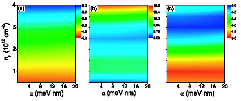
Figure 3: (Color online) (a) conventional spin Hall conductance component $\sigma_{yx}^{s0}$, (b) spin torque dipole component $\sigma_{yx}^{s\tau}$, and (c) the total spin Hall conductance $\sigma_{yx}^{s}$ (in unit of $e/4\pi$) as a function of Rashba coefficient $\alpha$ and hole density $n_{h}$ (contour plot).

Now we turn on the SIA Rashba term which is essential for understanding spin transport in strong spin-orbit coupling regime in experimental quantum well setup. Inclusion of $\alpha$-term in makes the analytic derivation of spin Hall conductance very tedious. Instead of doing that, we numerically obtain the eigenstates and eigen-energies of Hamiltonian (24), and substitute them in Eq. (18) and (20). After a $k$-integration with fermi wavevector pinned by the given hole density at zero temperature [see Fig. 1(b) for the relationship between HH fermi wavevectors and $\alpha$], the spin Hall conductance is therefore steadily calculated in a wide range of system parameters. Figures 3(a)-(c) summarize the behavior of the conventional, the spin-torque-dipole contributed, and the total spin Hall conductance, respectively, as a function of Rashba coefficient $\alpha$ and hole density $n_{h}$ (contour plot). Compared to the results without consideration of Rashba spin splitting (Fig. 2), the prominent new features occurred in Figs. 3 are: (i) The conventional term $\sigma_{yx}^{s0}$ and the spin torque dipole term $\sigma_{yx}^{s\tau}$ jump to much larger values upon switch on of Rashba spin splitting. This jump is caused by the presence of coupling between the two HH bands, which is absent without considering the SIA term; (ii) The amplitude of $\sigma_{yx}^{s\tau}$ becomes larger than that of conventional one $\sigma_{yx}^{s0}$ with a sign difference. In fact, the typical value of $\sigma_{yx}^{s0}$ in a wide range in ($\alpha,n_{h}$) parameter space is about ${\small\sim}\frac{-5e}{4\pi}$, while $\sigma_{yx}^{s\tau}$ is typically of ${\small\sim}\frac{10e}{4\pi}$, resulting in $\sigma_{yx}^{s}{\small\sim}\frac{5e}{4\pi}$. Thus overall the conserved spin Hall conductance changes a sign compared to the previous calculations based on conventional definition; (iii) The stripe in Figs. 3 reveals that the amplitude of intrinsic spin Hall conductance for 2DHG is insensitive to the amplitude of Rashba coefficient $\alpha$, which implies a universal character. The previous studiesSinova on a $k$-linear Rashba 2DEG system within the conventional definition of spin current have revealed a universal spin Hall conductance ($\sigma_{yx}^{s0}$) of $e/8\pi$. We have also calculated the conserved spin Hall conductance $\sigma_{yx}^{s}$ with the same model and found it to be $-e/8\pi$. Together with the above results for 2DHG, one can see the key role played by the spin torque dipole term, which tends to overwhelm the conventional spin conductance by the opposite contribution.

Since the LH bands are usually unoccupied by the holes in the experiments, and one can expect that in the weak Rshba spin splitting, the major contribution to the spin Hall conductance comes from the coupling between the two HH bands. In this case we can approximate the four-band Hamiltonian (24) by an effective two-band one. After a standard adiabatic elimination procedure, we obtain an effective two-band Hamiltonian $\bar{H}$ for heavy holes (in the strong confinement limit $k^{2}<\langle k_{z}^{2}\rangle$),

$$\bar{H}=\frac{\langle k_{z}^{2}\rangle}{2m_{HH}}+\frac{k^{2}}{2m^{\ast}}+i\beta(k_{-}^{3}\sigma_{+}-k_{+}^{3}\sigma_{-})$$ (30)

where $\beta=\frac{3}{8}\frac{\alpha(\langle k_{z}^{2}\rangle-4m_{LH}^{2}\alpha^{2})}{\langle k_{z}^{2}\rangle^{2}}$, $m_{HH,LH}=m/(\gamma_{1}\mp 2\gamma_{2})$, $m^{\ast}=2m_{HH}m_{LH}/(m_{HH}+m_{LH})$ is the reduced mass which is due to the proper account for the coupling between HH and LH bands, and $\sigma_{\pm}=\sigma_{x}\pm i\sigma_{y}$ are Pauli matrices. To reflect the angular momentum quantum numbers of the heavy holes, the conserved spin Hall current operator is defined by $\hat{\boldsymbol{\mathcal{J}}}_{s}=\frac{3}{2}\frac{\mathrm{d}(\hat{\mathbf{r}}\hat{s}_{z})}{\mathrm{d}t}$. Thus after an adiabatic projection onto the two HH bands, the Hamiltonian (24) is reduced to an effectice $k$-cubic Rashba model. In this case, we can derive an analytic expression for $\sigma_{yx}^{s}$ and its two components $\sigma_{yx}^{s0}$ and $\sigma_{yx}^{s\tau}$. The results at zero temperature are given by

$$\sigma_{yx}^{s0} =-\frac{9e}{32\pi}\frac{\gamma_{1}}{m\beta}(\frac{1}{k_{f}^{+}}-\frac{1}{k_{f}^{-}})$$

$$\sigma_{yx}^{s\tau} =\frac{27e}{32\pi}\frac{\gamma_{1}}{m\beta}(\frac{1}{k_{f}^{+}}-\frac{1}{k_{f}^{-}})-\frac{9e}{8\pi}$$ (31)

$$\sigma_{yx}^{s} =\frac{9e}{16\pi}\frac{\gamma_{1}}{m\beta}(\frac{1}{k_{f}^{+}}-\frac{1}{k_{f}^{-}})-\frac{9e}{8\pi}$$

where $k_{f}^{+}$ and $k_{f}^{-}$ are fermi wavevectors of the two HH bands. According to the experimentally accessible hole density $n_{h}$, these two fermi wave vectors can be expressed asLoss

$$k_{f}^{+,-} =\left[-\frac{1}{2}\left(\frac{\gamma}{2\beta}\right)^{2}\left(1-\sqrt{1-\left(\frac{2\beta}{\gamma}\right)^{2}4\pi n_{h}}\right)+3\pi n_{h}\right]^{1/2}$$

$$\mp\frac{1}{2}\frac{\gamma}{2\beta}\left(1-\sqrt{1-\left(\frac{2\beta}{\gamma}\right)^{2}4\pi n_{h}}\right).$$

where $\gamma=\hbar^{2}/2m^{\ast}$. In the limit $n_{h}<<(1/4\pi)(\gamma/2\beta)^{2}$, these fermi wavevectors have more simple forms: $k_{f}^{+,-}\approx\sqrt{2\pi n_{h}}\mp(2\beta/\gamma)\pi n_{h}$. In this case one gets $\sigma_{yx}^{s0}=-\frac{9e}{8\pi}$, $\sigma_{yx}^{s\tau}=\frac{9e}{4\pi}$, thus $\sigma_{yx}^{s}=\frac{9e}{8\pi}$. In general $\sigma_{yx}^{s}$ depends on the spin-orbit coupling and the fermi energy which is pinned by the hole density. For further illustration, we show in Fig. 4

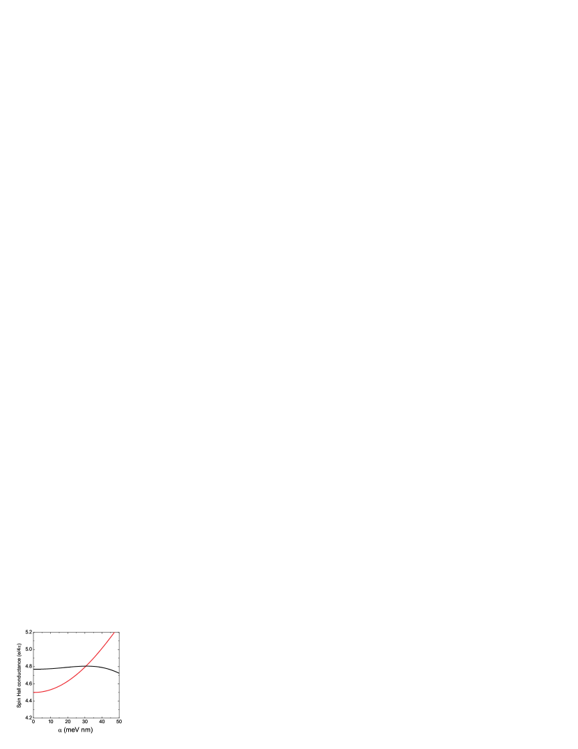
Figure 4: (Color online) conserved spin Hall conductivity $\sigma_{yx}^{s}$ as a function of Rashba coefficients $\alpha$ for $n_{h}=1.5\times 10^{12}$ cm^-2. The black line is the exact four-band result while the red line gives the approximate two-band result for the heavy holes.

the numerical results of conseved spin Hall conductance $\sigma_{yx}^{s}$ as a function of Rashba coefficient $\alpha$ for the four-band (black curve) and the approximate two-band (red curve) Hamiltonians. Note that the coefficient $\beta$ in Eq. (30) is obtained from $\alpha$ by the equation below Eq. (30). It reveals in Fig. 4 that the results from the two models agree reasonably in the experimentally relevant variation of spin-orbit coupling coefficient. When the value of spin splitting $\alpha k_{f}$ ($k_{f}$ characterizes fermi wavevector) is large enough to be comparable with the confinement characteristic energy $\langle k_{z}^{2}\rangle/2m$, then the deviation of the two-band approximation from the four-band calculation becomes obvious, which is featured in Fig. 4 by the fact that while the two-band $\sigma_{yx}^{s}$ increases monotonically as a function of $\alpha^{2}$ (which can also be seen from Eq. (31), the four-band spin Hall conductance displays a much weaker dependence of Rashba coefficient. Therefore we arrive at a conclusion that the neglect of HH-LH coupling is no longer valid for strong spin splitting and a more exact multi-band simulation is necessary for the general 2DHG systems.

VI Summary

In this article we have studied spin transport features in general spin-orbit coupled systems. Due to the spin-orbit coupling, the spin is not conserved by the occurrence of spin torque during its flow through the sample. Therefore, how to describe the spin transport within an intuitive drive-then-flow picture becomes an important issue. The key point clarified in this paper is as follows: (i) We have shown within the linear response formalism the necessity to include the spin torque dipole term in the expression of the spin current. The real advantage of our new definition of spin current lies in the fact that it provides a satisfactory description of spin transport in the bulk. With our new spin current, one can now use the spin continuity equation (6) to discuss spin accumulation in the bulk, e.g., by generating a non-uniform electric field or spatially modulating the spin Hall conductivity. Our new spin current vanishes in Anderson insulators either in equilibrium or in a weak electric field, which enables us to predict zero spin accumulation in such systems. More importantly, it possesses a conjugate force (spin force), so that spin transport can be fitted into the standard formalism of near equilibrium transport. The conventional spin current does not have a conjugate force, so it makes no sense even to talk about energy dissipation from that current. The existence of a conjugate force is crucial for the establishment of Onsager relations between spin transport and other transport phenomena, and its measurement will be important to thermodynamic and electric determination of the spin current. (ii) A general Kubo formula for the conserved spin transport coefficients, consisting of the conventional and spin-torque-dipole contrbutions, has been derived, which makes the practical bulk calculation to be feasible.

Based on the Kubo formula for the conserved spin current, we have analyzed in detail the spin Hall effect in 2DHG system with the parameters chosen to be relevant to recent experimental measurement on GaAs quantum well and modeled by the Hamiltonian consisting of a Luttinger spin-orbit coupling term and a SIA Rashba term. In the absence of Rashba spin splitting, the two HH (and LH) bands are degenerate and the non-zero spin Hall conductance only comes from HH-LH transition. In this case, we have derived an analytic expression for the conserved spin Hall conductance $\sigma_{yx}^{s}$ and its two components, the conventional one $\sigma_{yx}^{s0}$ and the spin torque dipole correction $\sigma_{yx}^{s\tau}$. These two components have been shown to compete each other, which is verified by a difference of sign between them. In the case that only the Luttinger term is taken into account, it has been found that the amplitude of $\sigma_{yx}^{s\tau}$ is much small than that of $\sigma_{yx}^{s0}$. In fact, the value of $\sigma_{yx}^{s0}$ is typically of $-\frac{0.8e}{4\pi}$ while $\sigma_{yx}^{s\tau}$ is about $\frac{0.2e}{4\pi}$. Thus in this case, the spin torque dipole correction to the spin Hall conductivity is relatively small. When the SIA Rashba spin splitting is turned on, we have found that there occurs a jump in amplitude for both $\sigma_{yx}^{s0}$ and $\sigma_{yx}^{s\tau}$. $\sigma_{yx}^{s0}$ changes now to take a typical value of $-\frac{5e}{4\pi}$ while $\sigma_{yx}^{s\tau}$ jumps to a characteristic value of $\frac{10e}{4\pi}$. Therefore, the presence of Rashba term not only stirs up a large enhancement of the total spin Hall conductivity and its two components, but also changes a fundamental sign for $\sigma_{yx}^{s}$ because the spin torque dipole correction now overwhelms the conventional contribution. This jump and a change of sign for $\sigma_{yx}^{s}$ comes from the HH-HH coupling, and therefore can be modeled by an effective two-band Hamiltonian which has been done in this paper by adiabatically eliminating the LH states and reducing the system to a $k$-cubic Rashba model with a dressed spin-orbit coupling coefficient [$\beta$ in Eq. (30)]. By a detailed comparison, furthermore, we have shown that this two-band $\sigma_{yx}^{s}$ displays a quadric dependence of original Rashba coefficient $\alpha$, while the exact four-band treatment shows a somewhat universal character for $\sigma_{yx}^{s}$. Thus the neglect of HH-LH coupling is no longer valid for strong spin splitting and a more exact multi-band simulation is necessary for the general 2DHG systems.

- (1) G.A. Prinz, Science 282, 1660 (1998); S.A. Wolf et al, Science 294, 1488 (2001).
- (2) Semiconductor Spintronics and Quantum Computation, edited by D.D. Awschalom, N. Sarmarth, and D. Loss (Springer-Verlag, Berlin, 2002).
- (3) I. Žutić, J. Fabian, and S.D. Sarma, Rev. Mod. Phys. 76, 323 (2004).
- (4) J. E. Hirsch, Phys. Rev. Lett. 83, 1834 (1999).
- (5) S. Zhang, Phys. Rev. Lett. 85, 393 (2000).
- (6) M.I. Dyakonov and V.I. Perel, JETP 33, 1053 (1971).
- (7) S. Murakami, N. Nagaosa, and S.C. Zhang, Science 301, 1348 (2003).
- (8) J. Sinova, D. Culcer, Q. Niu, N.A. Sinitsyn, T. Jungwirth, and A.H. MacDonald, Phys. Rev. Lett. 92, 126603 (2004).
- (9) Y.K. Kato et al., Science 306, 1910 (2004).
- (10) J. Wunderlich, B. Kaestner, J. Sinova, T. Jungwirth, Phys. Rev. Lett. 94, 047204 (2005).
- (11) V. Sih et al., Nature Phys. 1, 31 (2005).
- (12) Y. Yao and Z. Fang, Phys. Rev. Lett. 95, 156601 (2005).
- (13) S. Murakami, N. Nagaosa, and S. C. Zhang, Phys. Rev. Lett. 93, 156804 (2004).
- (14) E.I. Rashba, Phys. Rev. B 68, 241315(R) (2003). Actually is non-zero even in the presence of a confinement potential.
- (15) P. Zhang and Q. Niu, unpublished, cond-mat/0406436.
- (16) J. Shi, P. Zhang, D. Xiao, and Q. Niu, Phys. Rev. Lett. 96, 196602 (2006).
- (17) D. Culcer et al., Phys. Rev. Lett. 93, 046602 (2004).
- (18) P.-Q. Jin, Y.-Q. Li and F.-C. Zhang, preprint, condmat/0502231.
- (19) S. Murakami, N. Nagaosa, and S.-C. Zhang, Phys. Rev. B 69, 235206 (2004).
- (20) S. Zhang and Z. Yang, Phys. Rev. Lett. 94, 066602 (2005).
- (21) Q. Sun and X.C. Xie, Phys. Rev. B 72, 245305 (2005).
- (22) Y. Wang, K. Xia, Z.-B. Su, and Z. Ma, Phys. Rev. Lett. 96, 066601 (2006).
- (23) K. Nomura, J. Wunderlich, Jairo Sinova, B. Kaestner, A.H. MacDonald, T. Jungwirth, preprint, cond-mat/0508532.
- (24) W.-K. Tse, J. Fabian, I. Žutić, S. Das Sarma, Phys. Rev. B 72, 241303 (2005).
- (25) I. Žutić, J. Fabian, S. Das Sarma, Phys. Rev. Lett. 88, 066603 (2002); J. Fabian, I. Žutić, S. Das Sarma, Phys. Rev. B 66, 165301 (2002).
- (26) H.B. Casimir, Rev. Mod. Phys. 17, 843 (1945).
- (27) N. Sugimoto, S. Onoda, S. Murakami and N. Nagaosa, Phys. Rev. B 73, 113305 (2006).
- (28) B. Andrei Bernevig and S. C. Zhang, Phys. Rev. Lett. 95, 016801 (2005).
- (29) R. Winkler, Phys. Rev. B 62, 4245 (2000).
- (30) R. Winkler et. al, Phys. Rev. B 65, 155303 (2002).
- (31) J. Schliemann and D. Loss, Phys. Rev. B 71, 085308 (2005).