Elementary events of electron transfer in a voltage-driven quantum point contact

Abstract

We find that the statistics of electron transfer in a coherent quantum point contact driven by an arbitrary time-dependent voltage is composed of elementary events of two kinds: unidirectional one-electron transfers determining the average current and bidirectional two-electron processes contributing to the noise only. This result pertains at vanishing temperature while the extended Keldysh-Green’s function formalism in use also enables the systematic calculation of the higher-order current correlators at finite temperatures.

The most detailed description of the charge transfer in coherent conductors is a statistical one. At constant bias, the full counting statistics (FCS) of electron transfer art:LevitovLesovikJETP93 can be directly interpreted in terms of elementary events independent at different energies. The FCS approach is readily generalized to the case of a time-dependent voltage bias art:IvanovLevitovJETP93 ; art:LevitovJMath . The current fluctuations in coherent systems driven by a periodic voltage strongly depend on the shape of the driving art:LevitovNonstatAB , which frequently is not apparent in the average current art:Pedersen . The noise power, for instance, exhibits at low temperatures a piecewise linear dependence on the dc voltage with kinks corresponding to integer multiples of the ac drive frequency and slopes which depend on the shape and the amplitude of the ac component. This dependence has been observed experimentally in normal coherent conductors art:SchoelkopfPRL98 and diffusive normal metal–superconductor junctions art:KozhevnikovPRL00 .

The elementary events of charge transfer driven by a general time-dependent voltage have not been identified so far. The time dependence mixes the electron states at different energies art:Pedersen which makes this question both interesting and non-trivial. The first step in this research has been made in art:LeeLevitovCMat95 for a special choice of the time-dependent voltage. The authors have considered a superposition of overlapping Lorentzian pulses of the same sign (”solitons”), with each pulse carrying a single charge quantum. The resulting charge transfer is unidirectional with a binomial distribution of transmitted charges. The number of attempts per unit time for quasiparticles to traverse the junction is given by the dc component of the voltage, independent of the overlap between the pulses and their duration art:IvanovLeelevitovPRB97 . It has been shown that such superposition minimizes the noise reducing it to that of a corresponding dc bias. A microscopic picture behind the soliton pulses has been revealed only recently art:KlichLevitov06 . In contrast to a general voltage pulse which can in principle create a random number of electron-hole pairs with random directions, a soliton pulse at zero temperature always creates a single electron-hole pair with quasiparticles moving in opposite directions. One of the quasiparticles (say, electron) comes to the contact and takes part in the transport while the hole goes away. Therefore, soliton pulses can be used to create minimal excitation states with ”pure” electrons excited from the filled Fermi sea and no holes left below. The existence of such states can be probed by noise measurements art:KlichLevitov06 ; art:ButtikerPRB05 ; art:MuzykantskiiPRB05 .

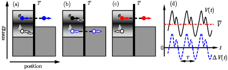
Figure 1: Schematic representation of elementary events: bidirectional (a, b) and unidirectional (c). Shifts of the effective chemical potential in the left lead due to time-dependent voltage drive are indicated by shading. For periodic drive, the dc voltage component [panel (d), dash-dotted line] describes unidirectional charge transfer, while the ac component (dashed curve) describes bidirectional events affecting the noise and higher-order even cumulants.

In this Letter, we do identify the independent elementary events for an arbitrary time-dependent driving applied to a generic conductor. Since generic conductor at low energies can be represented as a collection of independent transport channels, it is enough to specify elementary events for a single channel of transmission $T$. The answer is surprisingly simple. There are two kinds of such events: We call them bidirectional and unidirectional. In the course of a bidirectional event $k$ an electron-hole pair is created with probability $\sin^{2}({\alpha}_{k}/2)$, with $\alpha_{k}$ being determined by the details of the time-dependent voltage. The electron and hole move in the same direction reaching the scatterer. The charge transfer occurs if the electron is transmitted and the hole is reflected, or vice versa [Fig. 1(a,b)]. The probabilities of both outcomes, $TR$ ($R$ being reflection coefficient), are the same. Therefore, the bidirectional events do not contribute to the average current and odd cumulants of the charge transferred although they do contribute to the noise and higher-order even cumulants. A specific example of a bidirectional event for a soliton-antisoliton pulse was given in art:IvanovLeelevitovPRB97 .

The unidirectional events are the same as for a constant bias or a soliton pulse. They are characterized by chirality ${\kappa}_{l}=\pm 1$ which gives the direction of the charge transfer. An electron-hole pair is always created in the course of the event, with electron and hole moving in opposite directions [Fig. 1(c)]. Either electron (${\kappa}_{l}=1$) or hole (${\kappa}_{l}=-1$) passes the contact with probability $T$, thus contributing to the current.

Mathematically, the above description corresponds to the cumulant generating function $S({\chi})=S_{1}({\chi})+S_{2}({\chi})$, where

$$S_{1}=2\sum_{k}\ln\left[1+TR\sin^{2}\left(\frac{{\alpha}_{k}}{2}\right)(e^{i{\chi}}+e^{-i{\chi}}-2)\right]$$ (1)

and

$$S_{2}=2\sum_{l}\ln[1+T(e^{-i{\kappa}_{l}{\chi}}-1)]$$ (2)

are the contributions of the bidirectional and unidirectional events, respectively. Here ${\chi}$ is the counting field, and ${\alpha}_{k}$ and ${\kappa}_{l}$ are the parameters of the driving to be specified later. The sum in both formulas is over the set of corresponding events countability . The elementary events have been inferred from the form of the cumulant-generating function, as it has been done in art:events ; art:events1 .

The cumulant-generating function given by Eqs. (1) and (2), together with the interpretation, is the main result of this Letter. It holds at zero temperature only: since the elementary events are the electron-hole pairs created by the applied voltage, the presence of thermally excited pairs will smear the picture. Equations  (1) and (2) contain the complete ${\chi}$-field dependence in explicit form which allows for the calculation of higher-order cumulants and charge transfer statistics for arbitrary time-dependent voltage. The probability that $N$ charges are transmitted within the time of measurement is given by $P(N)=(2\pi)^{-1}\int_{-\pi}^{\pi}d{\chi}\exp[S({\chi})-iN{\chi}]$. Higher-order derivatives of $S$ with respect to ${\chi}$ are proportional to the cumulants of transmitted charge, or equivalently, to higher-order current correlators at zero frequency. The details of the driving are contained in the set of parameters $\{{\alpha}_{k}\}$ and separated from the ${\chi}$-field dependence. This opens an interesting possibility to excite the specific elementary processes and design the charge transfer statistics by appropriate time dependence of the applied voltage, with possible applications in production and detection of the many-body entangled states art:events ; art:BlatterPRB05 ; art:Beenakker .

Below we present the microscopic derivation of Eqs. (1) and (2). We neglect charging effects and assume instantaneous scattering at the contact with quasiparticle dwell times much smaller than the characteristic time scale of the voltage variations. The approach we use is the nonequilibrium Keldysh-Green’s function technique, extended to access the full counting statistics art:NazarovAnnPhys ; art:BelzigPRL01 ; art:BelzigInBook ; art:NazarovEPJB03 . The Green’s functions of the left ($1$) and right ($2$) leads are given by art:BelzigPRL01 ; art:BelzigInBook

$${\check{G}}_{1}=e^{-i{\chi}{\check{\tau}}_{1}/2}\begin{pmatrix}1&2{\tilde{h}}\\ 0&-1\end{pmatrix}e^{i{\chi}{\check{\tau}}_{1}/2},\quad{\check{G}}_{2}=\begin{pmatrix}1&2h\\ 0&-1\end{pmatrix},$$ (3)

where ${\check{\tau}}_{1}=\bigl{(}\begin{smallmatrix}0&1\\ 1&0\end{smallmatrix}\bigr{)}$ is a matrix in Keldysh($\,\check{}\,$) space. Hereafter we use a compact operator notation in which the time (or energy) indices are suppressed and the products are interpreted in terms of convolution over internal indices, e.g., $({\check{G}}_{1}{\check{G}}_{2})(t^{\prime},t^{\prime\prime})=\int dt_{1}{\check{G}}_{1}(t^{\prime},t_{1}){\check{G}}_{2}(t_{1},t^{\prime\prime})$ (and similar in the energy representation). The equilibrium Green’s function ${\check{G}}_{2}(t^{\prime}-t^{\prime\prime})$ depends only on time difference. In the energy representation ${\check{G}}_{2}({\cal E}^{\prime},{\cal E}^{\prime\prime})$ is diagonal in energy indices with $h({\cal E}^{\prime},{\cal E}^{\prime\prime})=\tanh({\cal E}^{\prime}/2{T_{e}})\;2\pi{\delta}({\cal E}^{\prime}-{\cal E}^{\prime\prime})$. Here the quasiparticle energy ${\cal E}$ is measured with respect to the chemical potential in the absence of the bias and ${T_{e}}$ is the temperature. The Green’s function ${\check{G}}_{1}(t^{\prime},t^{\prime\prime})$ depends on two time (or energy) arguments. It takes into account the effect of applied voltage $V(t)$ across the junction through the gauge transformation ${\tilde{h}}=UhU^{\dagger}$ which makes ${\check{G}}_{1}$ nondiagonal in energy representation. The unitary operator $U$ is given by $U(t^{\prime},t^{\prime\prime})=f(t^{\prime}){\delta}(t^{\prime}-t^{\prime\prime})$ in the time representation, where $f(t^{\prime})=\exp[-i\int_{0}^{t^{\prime}}eV(t)dt]$. The cumulant generating function $S({\chi})$ of the charge transfer through the junction is given by art:BelzigInBook ; art:NazarovSuperlatt99

$$S({\chi})=\mathop{\rm Tr}\nolimits\ln\left[{\check{1}}+\frac{T}{2}\left(\frac{{\{{\check{G}}_{1},{\check{G}}_{2}\}}}{2}-{\check{1}}\right)\right].$$ (4)

Here the trace and products of Green’s functions include both summation in Keldysh indices and integration over time (energy). For a dc voltage bias, ${\check{G}}_{1}$ and ${\check{G}}_{2}$ are diagonal in energy indices and $S({\chi})$ is readily interpreted in terms of elementary events independent at different energies art:BelzigInBook . To deduce the elementary events in the presence of time dependent voltage drive it is necessary to diagonalize ${\{{\check{G}}_{1},{\check{G}}_{2}\}}_{{\cal E}^{\prime}{\cal E}^{\prime\prime}}$. The diagonalization procedure is described in the following.

For the anticommutator of the Green’s functions we find ${\{{\check{G}}_{1},{\check{G}}_{2}\}}/2-{\check{1}}=-2\sin({\chi}/2)({\check{\cal A}}+{\check{\cal B}})$, with ${\check{\cal A}}=\bigl{(}\begin{smallmatrix}1&b\\ 0&0\end{smallmatrix}\bigr{)}\otimes A$, and ${\check{\cal B}}=\bigl{(}\begin{smallmatrix}0&-b\\ 0&1\end{smallmatrix}\bigr{)}\otimes B$. Here $A=(1-h{\tilde{h}})\sin({\chi}/2)+i(h-{\tilde{h}})\cos({\chi}/2)$, $B=(1-{\tilde{h}}h)\sin({\chi}/2)+i(h-{\tilde{h}})\cos({\chi}/2)$, $b=-i\cot({\chi}/2)$, and $\otimes$ is the tensor product. Since ${\check{\cal A}}{\check{\cal B}}={\check{\cal B}}{\check{\cal A}}=0$, the operators ${\check{\cal A}}$ and ${\check{\cal B}}$ commute and satisfy for integer $n$: $({\check{\cal A}}+{\check{\cal B}})^{n}=\bigl{(}\begin{smallmatrix}1&b\\ 0&0\end{smallmatrix}\bigr{)}\otimes A^{n}+\bigl{(}\begin{smallmatrix}0&-b\\ 0&1\end{smallmatrix}\bigr{)}\otimes B^{n}$. Therefore, $S({\chi})$ given by Eq. (4) reduces to

$$S=\mathop{\rm Tr}\nolimits\ln\left[1-T\sin\left(\frac{{\chi}}{2}\right)A\right]+\mathop{\rm Tr}\nolimits\ln\left[1-T\sin\left(\frac{{\chi}}{2}\right)B\right].$$ (5)

A further simplification of $S({\chi})$ is possible in the zero temperature limit, in which the hermitian $h$-operators are involutive: $h^{2}={\tilde{h}}^{2}=1$. The operators $h{\tilde{h}}$ and ${\tilde{h}}h$ are mutually inverse and commute with each other. Because $h{\tilde{h}}$ is unitary, it has the eigenvalues of the form $e^{i{\alpha}_{k}}$ with real ${\alpha}_{k}$, and possesses an orthonormal eigenbasis $\{{\mathrm{v}}_{{\alpha}_{k}}\}$. The typical eigenvalues of $h{\tilde{h}}$ (or ${\tilde{h}}h$) appear in pairs $e^{\pm i{\alpha}}$ with the corresponding eigenvectors ${\mathrm{v}}_{\alpha}$ and ${\mathrm{v}}_{-{\alpha}}=h{\mathrm{v}}_{\alpha}$. In the basis $({\mathrm{v}}_{\alpha},{\mathrm{v}}_{-{\alpha}})$ operators $h{\tilde{h}}$ and ${\tilde{h}}h$ are diagonal and given by $h{\tilde{h}}=\mathop{\rm diag}\nolimits(e^{i{\alpha}},e^{-i{\alpha}})$ and ${\tilde{h}}h=\mathop{\rm diag}\nolimits(e^{-i{\alpha}},e^{i{\alpha}})$. The eigensubspaces $\mathop{\rm span}\nolimits({\mathrm{v}}_{\alpha},{\mathrm{v}}_{-{\alpha}})$ of the anticommutator ${\{h,{\tilde{h}}\}}$ are invariant with respect to $h$, ${\tilde{h}}$, and $A$ because of ${[h,{\{h,{\tilde{h}}\}}]}={[{\tilde{h}},{\{h,{\tilde{h}}\}}]}=0$. The operators $h$ and ${\tilde{h}}$ are anti-diagonal in the basis $({\mathrm{v}}_{\alpha},{\mathrm{v}}_{-{\alpha}})$, with matrix components $h_{12}=1$, $h_{21}=1$, ${\tilde{h}}_{12}=e^{-i{\alpha}}$, and ${\tilde{h}}_{21}=e^{i{\alpha}}$. The operator $A$ can be diagonalized in invariant subspaces, with typical eigenvalues given by

$$\mathop{\rm ev}\nolimits A=2\sin({\alpha}/2)\bigg{(}\sin({\alpha}/2)\sin({\chi}/2)\\ \pm i\sqrt{1-\sin^{2}({\alpha}/2)\sin^{2}({\chi}/2)}\bigg{)}.$$ (6)

Similarly, we obtain $\mathop{\rm ev}\nolimits B=\mathop{\rm ev}\nolimits A$. From Eqs. (5) and (6) we recover the generating function $S_{1}$ given by Eq. (1), which is associated with the paired eigenvalues $e^{\pm i{\alpha}_{k}}$.

There are, however, some special eigenvectors of $h{\tilde{h}}$ which do not appear in pairs. The pair property discussed above was based on the assumption that ${\mathrm{v}}_{\alpha}$ and $h{\mathrm{v}}_{\alpha}={\mathrm{v}}_{-{\alpha}}$ are linearly independent vectors. In the special case, these vectors are the same apart from a coefficient. Therefore, the special eigenvectors of $h{\tilde{h}}$ are the eigenvectors of both $h$ and ${\tilde{h}}$ with eigenvalues ${\pm 1}$. This means that the special eigenvectors posses chirality, with positive (negative) chirality defined by $h{\mathrm{v}}={\mathrm{v}}$ and ${\tilde{h}}{\mathrm{v}}=-{\mathrm{v}}$ ($h{\mathrm{v}}=-{\mathrm{v}}$ and ${\tilde{h}}{\mathrm{v}}={\mathrm{v}}$). From Eq. (5) we obtain the generating function $S_{2}({\chi})$ given by Eq. (2), where $l$ labels the special eigenvectors and ${\kappa}_{l}$ is the chirality.

In the following we focus on a periodic driving $V(t+{\tau})=V(t)$ with the period ${\tau}=2\pi/{\omega}$, for which the eigenvalues of $h{\tilde{h}}$ can be easily obtained by matrix diagonalization. The operator ${\tilde{h}}$ couples only energies which differ by an integer multiple of ${\omega}$, which allows to map the problem into the energy interval $0<{\cal E}<{\omega}$ while retaining the discrete matrix structure in steps of ${\omega}$. Therefore, the trace operation in Eq. (4) becomes an integral over ${\cal E}$ and the trace in discrete matrix indices. The operator $h{\tilde{h}}$ in the energy representation is given by $(h{\tilde{h}})_{nm}({\cal E})=\mathop{\rm sign}\nolimits({\cal E}+n{\omega})\sum_{k}{\tilde{f}}_{n+k}{\tilde{f}}_{m+k}^{*}\mathop{\rm sign}\nolimits({\cal E}-k{\omega}-e{\bar{V}})$, with ${\tilde{f}}_{n}=(1/{\tau})\int_{-{\tau}/2}^{{\tau}/2}dt\;e^{-i\int_{0}^{t}dt^{\prime}\;e{\Delta V}(t^{\prime})}e^{in{\omega}t}$. Here ${\bar{V}}=(1/{\tau})\int V(t)dt$ is the dc voltage offset and ${\Delta V}(t)=V(t)-{\bar{V}}$ is the ac voltage component. The coefficients ${\tilde{f}}_{n}$ satisfy $\sum_{k}{\tilde{f}}_{n+k}{\tilde{f}}_{m+k}^{*}={\delta}_{nm}$ and $\sum_{n}n|{\tilde{f}}_{n}|^{2}=0$.

To evaluate $S({\chi})$ for a given periodic voltage drive $V(t)$ it is necessary to diagonalize $(h{\tilde{h}})_{nm}({\cal E})$. First we analyze the contribution of typical eigenvalues $e^{\pm i{\alpha}}$. The matrix $(h{\tilde{h}})_{nm}({\cal E})$ is piecewise constant for ${\cal E}\in(0,{\omega}_{1})$ and ${\cal E}\in({\omega}_{1},{\omega})$, where ${\omega}_{1}=e{\bar{V}}-N{\omega}$ and $N=\lfloor e{\bar{V}}/{\omega}\rfloor$ is the largest integer less than or equal $e{\bar{V}}/{\omega}$. The eigenvalues $e^{\pm i{\alpha}_{kL(R)}}$ of $(h{\tilde{h}})_{nm}$ are calculated for ${\cal E}\in(0,{\omega}_{1})$ [${\cal E}\in({\omega}_{1},{\omega})$] using finite-dimensional matrices, with the cutoff in indices $n$ and $m$ being much larger than the characteristic scale on which $|{\tilde{f}}_{n}|$ vanish. Further increase of the size of matrix just brings more eigenvalues with ${\alpha}_{k}=0$ which do not contribute to $S({\chi})$, and does not change the rest with ${\alpha}_{k}\neq 0$. This is a signature that all important Fourier components of the drive are taken into account. The eigenvalues $e^{\pm i{\alpha}_{kL(R)}}$ give rise to two terms, $S_{1}=S_{1L}+S_{1R}$, with

$$S_{1L,R}({\chi})=M_{L,R}\sum_{k}\ln[1+TR\sin^{2}({\alpha}_{kL,R}/2)\\ \times(e^{i{\chi}}+e^{-i{\chi}}-2)].$$ (7)

Here $M_{L}=t_{0}{\omega}_{1}/\pi$, $M_{R}=t_{0}({\omega}-{\omega}_{1})/\pi$, and $t_{0}$ is the total measurement time which is much larger than ${\tau}$ and the characteristic time scale on which the current fluctuations are correlated.

The special eigenvectors all have the same chirality which is given by the sign of the dc offset ${\bar{V}}$. For $e{\bar{V}}>0$, there are $N_{1}=N+1$ special eigenvectors for ${\cal E}\in(0,{\omega}_{1})$ and $N_{2}=N$ for ${\cal E}\in({\omega}_{1},{\omega})$. Because $e{\bar{V}}=N_{1}{\omega}_{1}+N_{2}({\omega}-{\omega}_{1})$, the effect of the special eigenvectors is the same as of the dc bias

$$S_{2}({\chi})=\frac{t_{0}e{\bar{V}}}{\pi}\ln[1+T(e^{-i{\chi}}-1)].$$ (8)

Comparing Eqs. (2) and (8) we see that unidirectional events for periodic drive are uncountable. The summation in Eq. (2) stands both for the energy integration in the interval ${\omega}$ and the trace in the discrete matrix indices. In the limit of a single pulse ${\omega}\to 0$ unidirectional events remain uncountable for a generic voltage, while being countable, e.g., for soliton pulses carrying integer number of charge quanta art:IvanovLeelevitovPRB97 .

Equations (7) and (8) determine the charge transfer statistics at zero temperature for an arbitrary periodic voltage applied. The generating function consists of a binomial part ($S_{2}$) which depends on the dc offset ${\bar{V}}$ only, and a contribution of the ac voltage component ($S_{1}$) [Fig. 1(d)]. The latter is the sum of two terms which depend on the number of unidirectional attempts per period $e{\bar{V}}/{\omega}$. The simplest statistics is obtained for an integer number of attempts for which $S_{1L}$ vanishes art:IvanovLevitovJETP93 . The Fourier components of the optimal Lorentzian pulses $V_{L}(t)=(2{\tau}_{L}/e)\sum_{k}[(t-k{\tau})^{2}+{\tau}_{L}^{2}]^{-1}$ of width ${\tau}_{L}>0$ are given by ${\tilde{f}}_{-1}=-e^{-2\pi{\tau}_{L}/{\tau}}$, ${\tilde{f}}_{n}=e^{-2\pi n{\tau}_{L}/{\tau}}-e^{-2\pi(n+2){\tau}_{L}/{\tau}}$ for $n\geq 0$, and ${\tilde{f}}_{n}=0$ otherwise. In this case $S_{1L}=S_{1R}=0$ and the statistics is exactly binomial with one electron-hole excitation per period, in agreement with Refs. art:IvanovLeelevitovPRB97 ; art:KlichLevitov06 .

Figure 2: The probability of elementary events for harmonic drive with amplitude $V_{0}$ (upper panel). With increasing amplitude more and more eigenvalues ${\alpha}_{k}$ come into play and contribute to transport. The derivative of the noise power with respect to $V_{0}$ (—) decomposed into contributions (– –) of elementary events (lower panel).

The elementary events at zero temperature can be probed by noise measurements. For example, in the case of an ac drive with ${\bar{V}}=0$, only bidirectional events of $R$-type remain [$S({\chi})=S_{1R}({\chi})$]. Both the number of events and their probabilities increase with increasing the driving amplitude $V_{0}$, which results in the characteristic oscillatory change of the slope of the current noise power $P_{I}=(4e^{2}{\omega}/\pi)T(1-T)\sum_{k}\sin^{2}({\alpha}_{k}/2)$. The decomposition of $\partial P_{I}/\partial V_{0}$ into contributions of elementary events for harmonic drive is shown in Fig. 2.

Our method also enables the efficient and systematic analytic calculation of the higher-order cumulants at finite temperatures. They can be obtained directly from Eq. (5) by expansion in the counting field to the certain order before taking the trace. The trace of a finite number of terms can be taken in the original basis in which ${\check{G}}_{1}$ and ${\check{G}}_{2}$ are defined. The details of this approach will be given elsewhere. However, the formulas obtained (as a function of $\{{\tilde{f}}_{n}\}$) can not be interpreted as elementary events term by term. To identify the elementary events it is necessary to find $S({\chi})$ which requires full expansion or diagonalization, as presented above.

In conclusion, we have studied the statistics of the charge transfer in a quantum point contact driven by time-dependent voltage. We have deduced the elementary transport processes at zero temperature from an analytical result for the cumulant generating function. The transport consists of unidirectional and bidirectional charge transfer events which can be interpreted in terms of electrons and holes which move in opposite and the same directions, respectively. Unidirectional events account for the net charge transfer and are described by binomial cumulant generating function which depends on the dc voltage offset. Bidirectional events contribute only to even cumulants of charge transfer at zero temperature. They are created with probability which depends on the shape of the ac voltage component. The statistics of charge transfer is the simplest for an integer number of attempts for quasiparticles to traverse the junction. This results in photon-assisted effects in even-order cumulants as a function of a dc offset. The approach we have used also allows for the systematic calculation of higher-order cumulants at finite temperatures.

We acknowledge valuable discussions with L. S. Levitov and C. Bruder. This work has been supported by the Swiss NSF and NCCR ”Nanoscience” (MV), the DFG through SFB 513 and the Landesstiftung Baden-Württemberg (WB).

References

- (1) L. S. Levitov and G. B. Lesovik, Pis’ma Zh. Eksp. Teor. Fiz. 58, 225 (1993) [JETP Lett. 58, 230 (1993)].
- (2) D. A. Ivanov and L. S. Levitov, Pis’ma Zh. Eksp. Teor. Fiz. 58, 450 (1993) [JETP Lett. 58, 461 (1993)].
- (3) L. S. Levitov, H.-W. Lee, and G. B. Lesovik, J. Math. Phys. 37, 4845 (1996).
- (4) G. B. Lesovik and L. S. Levitov, Phys. Rev. Lett. 72, 538 (1994).
- (5) M. H. Pedersen and M. Büttiker, Phys. Rev. B 58, 12993 (1998).
- (6) R. Schoelkopf et al., Phys. Rev. Lett. 80, 2437 (1998); L.-H. Reydellet et al., Phys. Rev. Lett. 90, 176803 (2003).
- (7) A. A. Kozhevnikov, R. J. Schoelkopf, and D. E. Prober, Phys. Rev. Lett. 84, 3398 (2000).
- (8) H.-W. Lee and L. S. Levitov, cond-mat/9507011.
- (9) D. A. Ivanov, H.-W. Lee, and L. S. Levitov, Phys. Rev. B 56, 6839 (1997).
- (10) J. Keeling, I. Klich, and L. S. Levitov, Phys. Rev. Lett. 97, 116403 (2006).
- (11) N. d’Ambrumenil and B. Muzykantskii, Phys. Rev. B 71, 045326 (2005).
- (12) V. S. Rychkov, M. L. Polianski, and M. Büttiker, Phys. Rev. B 72, 155326 (2005); M. L. Polianski, P. Samuelsson, and M. Büttiker, ibid. 72, R161302 (2005).
- (13) The set of the unidirectional events is not necessary countable, see below.
- (14) J. Tobiska and Yu. V. Nazarov, Phys. Rev. B 72, 235328 (2005).
- (15) A. Di Lorenzo and Yu. V. Nazarov, Phys. Rev. Lett. 94, 210601 (2005).
- (16) A. V. Lebedev, G. B. Lesovik, and G. Blatter, Phys. Rev. B 72, 245314 (2005).
- (17) C. W. J. Beenakker, in Proc. Int. School Phys. E. Fermi, Vol. 162 (IOS Press, Amsterdam, 2006); L. Faoro, F. Taddei, and R. Fazio, Phys. Rev. B 69, 125326 (2004).
- (18) Yu. V. Nazarov, Ann. Phys. (Leipzig) 8, SI-193 (1999).
- (19) Yu. V. Nazarov and M. Kindermann, Eur. Phys. J. B 35, 413 (2003).
- (20) W. Belzig and Yu. V. Nazarov, Phys. Rev. Lett. 87, 197006 (2001).
- (21) W. Belzig, in Quantum Noise in Mesoscopic Physics, NATO ASI Series II, edited by Yu. V. Nazarov (Kluwer, Dordrecht, 2003), Vol. 97, p. 463.
- (22) Yu. V. Nazarov, Superlattices Microstruct. 25, 1221 (1999).