Limits of the upper critical field in dirty two-gap superconductors

Abstract

An overview of the theory of the upper critical field in dirty two-gap superconductors, with a particular emphasis on MgB₂ is given. We focus here on the maximum $H_{c2}$ which may be achieved by increasing intraband scattering, and on the limitations imposed by weak interband scattering and paramagnetic effects. In particular, we discuss recent experiments which have recently demonstrated ten-fold increase of $H_{c2}$ in dirty carbon-doped films as compared to single crystals, so that the $H_{c2}(0)$ parallel to the ab planes may approach the BCS paramagnetic limit, $H_{p}[T]=1.84T_{c}[K]\simeq 60-70T$. New effects produced by weak interband scattering in the two-gap Ginzburg-Landau equations and $H_{c2}(T)$ in ultrathin MgB₂ films are addressed.

I Introduction

It is now well established that superconductivity in MgB₂ with the unexpectedly high critical temperature $T_{c}\approx 40$K mgb2 , is due to strong electron-phonon interaction with in-plane boron vibration modes. Extensive ab-initio calculations tg1 ; tg2 ; tg3 , along with many experimental evidences from STM, point contact, and Raman spectroscopy, heat capacity, magnetization and rf measurements rev1 ; rev2 unambiguously indicate that MgB₂ exhibits two-gap s-wave superconductivity suhl ; moskal . MgB₂ has two distinct superconducting gaps: the main gap $\Delta_{\sigma}(0)\approx 7.2$mV, which resides on the 2D cylindrical parts of the Fermi surface formed by in-plane $\sigma$ antibonding $p_{xy}$ orbitals of B, and the smaller gap $\Delta_{\pi}(0)\approx 2.3$mV on the 3D tubular part of the Fermi surface formed by out-of-plane $\pi$ bonding and antibonding $p_{z}$ orbitals of B.

The discovery of MgB₂ has renewed interest in new effects of two-gap superconductivity, motivating different groups to take closer looks at other known materials, such as YNi₂B₂C and LuNi₂B₂C borocarbides borocarb Nb₃Sn nb3sn , or NbSe₂ nb2se , heavy-fermion heavyferm and organic organsc superconductors, for which evidences of the two gap behavior have been reported. However, several features of MgB₂ set it apart from other two-gap superconductors. Not only does MgB₂ have the highest $T_{c}$ among all non-cuprate superconductors, it also has two coexisting order parameters $\Psi_{\sigma}=\Delta_{\sigma}\exp(i\theta_{1})$ and $\Psi_{\pi}=\Delta_{\pi}\exp(i\theta_{2})$, which are weakly coupled. The latter is due to the fact that the $\sigma$ and $\pi$ bands are formed by two orthogonal sets of in-plane and out-of-plane atomic orbitals of boron, so all overlap integrals, which determine matrix elements of interband coupling and interband impurity scattering are strongly reduced mazimp . This feature can result in new effects, which are very important both for the physics and applications of MgB₂. Indeed, two weakly coupled gaps result in intrinsic Josephson effect, which can manifest itself in low-energy interband Josephson plasmons (the Legget mode) legget with frequencies smaller than $\Delta_{\pi}/\hbar$. Moreover, strong static electric fields and currents can decouple the bands due to formation of interband textures of $2\pi$ planar phase slips in the phase difference $\theta(x)=\theta_{1}-\theta_{2}$ text1 ; text2 well below the global depairing current. In turn, the weakness of interband impurity scattering makes it possible to radically increase the upper critical field $H_{c2}$ by selective alloying of Mg and B sites with nonmagnetic impurities.

Despite the comparatively high $T_{c}$, the upper critical field of MgB₂ single crystals is rather low and anisotropic with $H_{c2}^{\perp}(0)\simeq 3-5T$ and $H_{c2}^{||}(0)\simeq 15-19T$ of rev1 ; rev2 , where the indices $\perp$ and $||$ correspond to the magnetic field H perpendicular and parallel to the ab plane, respectively. Since these $H_{c2}$ values are significantly lower than $H_{c2}(0)\simeq 30$T for Nb₃Sn orlando ; arno , there had been initial scepticism about using MgB₂ as a high-field superconductor, until several groups undertook the well-established procedure of $H_{c2}$ enhancement by alloying MgB₂ with nonmagnetic impurities. The results of high-field measurements on dirty MgB₂ films and bulk samples has shown up to ten-fold increase of $H_{c2}^{\perp}$ as compared to single crystals h1 ; h2 ; h3 ; h4 ; h5 ; h6 ; h7 ; h8 ; h9 ; h10 ; h11 ; h12 , particularly in carbon-doped thin films h9 made by hybrid physico-chemical vapor deposition penn . This unexpectedly strong enhancement of $H_{c2}(T)$ results from its anomalous upward curvature, rather different from that of $H_{c2}(T)$ for one-gap dirty superconductors agork ; dege ; whh ; maki . As shown in Fig. 1, $H_{c2}$ of MgB₂ C-doped films has already surpassed $H_{c2}$ of Nb₃Sn, which could make cheap and ductile MgB₂ an attractive material for high field applications ap1 .

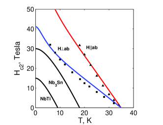
Figure 1: $H_{c2}(T)$ for carbon-doped MgB₂ films h9 in comparison with NbTi and Nb₃Sn. The red and blue lines show fits from Eq. (19) with $g=0.045$

.

This radical enhancement of $H_{c2}$ shown in Fig. 1 is indeed assisted by the features of two-gap superconductivity in MgB₂. Fig. 2 gives another example of $H_{c2}(T)$ for a fiber-textured film h6 , which exhibits an upward curvature of $H_{c2}(T)$ for $H||c$. This behavior of $H_{c2}(T)$ and the anomalous temperature-dependent anisotropy ratio $\Gamma(T)=H_{c2}^{||}(T)/H_{c2}^{\perp}(T)$ are different from that of the one-gap theory in which the $H_{c2}(T)$ has a downward curvature, while the slope $H_{c2}^{\prime}=dH_{c2}/dT$ at $T_{c}$ is proportional to the normal state residual resistivity $\rho_{n}$, and $H_{c2}(0)=0.69T_{c}H_{c2}^{\prime}$ agork ; dege ; whh ; maki . However, the behavior of $H_{c2}(T)$ in MgB₂ can be explained by the two-gap theory in the dirty limit based on either Usadel equations ag ; gk or Eliashberg equations borocarb ; carb .

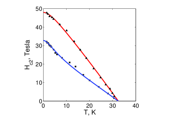
Figure 2: $H_{c2}(T)$ of a fiber-textured MgB₂ film h6 both parallel (triangles) and parallel (squares) to the ab planes. The solid lines show calculations from Eq. (19) with $g=0.065$, $D_{\pi}\ll D_{\sigma}^{(ab)}$ for $H||c$ and $D_{\pi}=0.19(D_{\sigma}^{(c)}D_{\sigma}^{(ab)})^{1/2}$ for $H\perp c$.

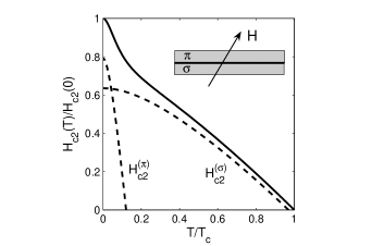
Figure 3: The mechanism of the upward curvature of $H_{c2}(T)$ illustrated by the bilayer toy model shown in the inset. The dashed curves show $H_{c2}(T)$ calculated for $\sigma$ and $\pi$ films in the one-gap dirty limit with the BCS coupling constants $\lambda_{\sigma}=0.81$, $\lambda_{\pi}=0.285$, and $D_{\pi}=0.1D_{\sigma}$. The solid curve shows $H_{c2}(T)$ calculated from Eq. (IV) of the two-gap dirty limit theory for the BCS matrix constants from Ref. goluba

The behavior of $H_{c2}(T)$ can be qualitatively understood using a simple bilayer model shown in Fig. 3, which captures the physics of two-gap superconductivity in MgB₂, and suggests ways by which $H_{c2}$ can be further increased. Indeed, MgB₂ can be mapped onto a bilayer in which two thin films corresponding to $\sigma$ and $\pi$ bands are separated by a Josephson contact, which models the interband coupling. The global $H_{c2}(T)$ of the such weakly-coupled bilayer is mostly determined by the film with the highest $H_{c2}$, even if $T_{c}^{(\sigma)}$ and $T_{c}^{(\pi)}$ are very different. For example, if the $\pi$ film is much dirtier than the $\sigma$ film then $H_{c2}^{(\sigma)}$ dominates at higher T, but at lower temperatures the $\pi$ film takes over, resulting in the upward curvature of $H_{c2}(T)$. If the $\sigma$ film is dirtier, the $\pi$ film only results in a slight shift of the $H_{c2}$ curve and a reduction of the slope $H_{c2}^{\prime}$ near $T_{c}$.

The bilayer model also clarifies the anomalous angular dependence of $H_{c2}(\alpha,T)$ for ${\bf H}$ inclined by the angle $\alpha$ with respect to the c-axis (parallel to the film normal in Fig. 3) note . In this case both $H_{c2}^{(\sigma)}(\alpha,T)$ and $H_{c2}^{(\pi)}(\alpha,T)$ depend on $\alpha$ according to the temperature-independent one-gap scaling $H_{c2}(\alpha)=H_{c2}(0,T)/\sqrt{\cos^{2}\alpha+\epsilon\sin^{2}\alpha}$ gork ; bul , but with very different effective mass ratios $\epsilon=m_{ab}/m_{c}$ for each film. Because the $\sigma$ band is much more anisotropic than the $\pi$ band, $\epsilon_{\sigma}\ll 1$, and $\epsilon_{\pi}\sim 1$ anz1 ; anz2 , the one-gap angular scaling for the global $H_{c2}(\alpha,T)$ breaks down. For example, in the case shown in Fig. 3, $H_{c2}(T)$ is anisotropic at higher T, but at lower T, the nearly isotropic $\pi$ band reduces the overall anisotropy of $H_{c2}$, so the ratio $\Gamma(T)=H_{c2}^{||}(T)/H_{c2}^{\perp}(T)$ decreases as T decreases. This is characteristic of many dirty MgB₂ films like the one shown in Fig. 2, for which the $\pi$ band is typically much dirtier than the $\sigma$ band. By contrast, in clean MgB₂ single crystals $\Gamma(T)$ increases from $\simeq 2-3$ near $T_{c}$ to $\simeq 5-6$ at $T\ll T_{c}$ a1 ; a2 ; a3 ; a4 ; a5 ; a6 ; a7 ; a8 ; a9 ; a10 ; a11 . This behavior was explained by two-gap effects in the clean limit vgk ; dahm .

Fig. 3 suggests that $H_{c2}(T)$ of MgB₂ can be significantly increased at low T by making the $\pi$ band much dirtier than the main $\sigma$ band. This could be done by disordering the Mg sublattice, thus disrupting the $p_{z}$ boron out-of-plane orbitals, which form the $\pi$ band. Achieving high $H_{c2}$ requires that both $\sigma$ and $\pi$ bands are in the dirty limit. Yet, making the $\pi$ band much dirtier than the $\sigma$ band provides a ”free boost” in $H_{c2}$ without too much penalty in $T_{c}$ suppression due to pairbreaking interband scattering or band depletion due to doping depl1 ; depl2 . In fact, the interband scattering is weak for the same reason that $\Psi_{\sigma}$ and $\Psi_{\pi}$ are weakly coupled, which may enable alloying MgB₂ with more impurities to achieve higher $H_{c2}$. Systematic incorporation of impurities in MgB₂ has not been yet achieved because the complex substitutional chemistry of MgB₂ is still poorly understood chem1 ; chem2 ; chem3 ; chem4 . Several groups have reported a significant increase in $H_{c2}$ by irradiation with protons prot , neutrons neut1 ; neut2 or heavy ions asu , but so far the carbon impurities have been the most effective to provide the huge $H_{c2}$ enhancement shown in Figs. 1 and 2. The effect of carbon on different superconducting properties can be rather complex carb1 ; carb2 ; carb3 and still far from being fully understood. Yet given the indisputable benefits of carbon alloying, one can pose the basic question: how far can $H_{c2}$ be further increased?

The bilayer model suggests that $H_{c2}$ increases if intraband scattering is enhanced. However, because intraband impurity scattering causes an admixture of pairbreaking interband scattering, the first question is to what extent weak interband scattering in MgB₂ can limit $H_{c2}$. Another important question is how far is the observed $H_{c2}$ from the paramagnetic limit $H_{p}$. In the BCS theory $H_{p}$ is defined by the condition: $\mu_{B}H_{p}^{BCS}=\Delta/\sqrt{2}$, or $H_{p}^{BCS}[T]=1.86T_{c}[K]$ par3 , where $\mu_{B}$ is the Bohr magneton. For $T_{c}=35K$, this yields $H_{p}=65$T, not that far from the zero-field $H_{c2}^{||}(0)$ in Figs. 1 and 2. However, the BCS model underestimates $H_{p}$, which is significantly enhanced by strong electron-phonon coupling par4 :

$$H_{p}\simeq(1+\lambda_{ep})H_{p}^{BCS},$$ (1)

where $\lambda_{ep}$ is the electron-phonon constant. Taking $\lambda_{ep}\approx 1$ for the $\sigma$ band tg1 ; tg2 , we obtain $H_{p}\sim 130$T, so there still a large room for increasing $H_{c2}$ by optimizing the intra and interband impurity scattering. For instance, increasing $H_{c2}^{\prime}$ to a rather common for many high field superconductors value of 2T/K (much lower than $H_{c2}^{\prime}\simeq 5-14$T/K for PbMo₆S₈ pb ) could drive $H_{c2}$ of MgB₂ with $T_{c}\simeq 35K$ above 70T. In the following we give a brief overview of recent results in the theory of dirty two-gap superconductors focusing on new effects brought by weak interband scattering and paramagnetic effects. The main conclusion is that, although interband scattering in MgB₂ is indeed weak, it cannot be neglected in calculations of $H_{c2}(T)$. We will also address the crossover from the orbitally-limited to the paramagnetically limited $H_{c2}$ in a two-gap superconductor.

II Tho-gap superconductors in the dirty limit

We regard MgB₂ as a dirty anisotropic superconductor with two sheets 1 and 2 of the Fermi surface on which the superconducting gaps take the values $\Delta_{1}$ and $\Delta_{2}$, respectively (indices 1 and 2 correspond to $\sigma$ and $\pi$ bands). Although the $\sigma$ band is anisotropic, MgB₂ is not a layered material layer1 ; layer2 , so the continuum BCS theory is applicable because the c-axis coherence length $\xi_{c}$ is much longer than the spacing between the boron planes $\sim 3.5\AA$. Indeed, even for $H_{c2}^{\perp}(0)=40$T and $H_{c2}^{||}(0)=60$T in Fig. 1, the anisotropic Ginzburg-Landau (GL) theory gork gives $\xi_{c}=(\phi_{0}H_{c2}^{\perp}/2\pi)^{1/2}/H_{c2}^{||}\approx 19\AA$. Strong coupling in MgB₂ should be described by the Eliashberg equations carb , but we consider here manifestations of intra and interband scattering and paramagnetic effects in $H_{c2}$ using the more transparent two-gap Usadel equations ag

$$\omega f_{1}-\frac{D_{1}^{\alpha\beta}}{2}[g_{1}\Pi_{\alpha}\Pi_{\beta}f_{1}-f_{1}\nabla_{\alpha}\nabla_{\beta}g_{1}]$$

$$=\Psi_{1}g_{1}+\gamma_{12}(g_{1}f_{2}-g_{2}f_{1})\qquad$$ (2)

$$\omega f_{2}-\frac{D_{2}^{\alpha\beta}}{2}[g_{2}\Pi_{\alpha}\Pi_{\beta}f_{2}-f_{2}\nabla_{\alpha}\nabla_{\beta}g_{2}]$$

$$=\Psi_{2}g_{2}+\gamma_{21}(g_{2}f_{1}-g_{1}f_{2}),\qquad$$ (3)

Here the Usadel Green’s functions $f_{m}({\bf r},\omega)$ and $g_{m}({\bf r},\omega)$ in the m-th band depend on ${\bf r}$ and the Matsubara frequency $\omega=\pi T(2n+1)$, $D_{m}^{\alpha\beta}$ are the intraband diffusivities due to nonmagnetic impurity scattering, $2\gamma_{mm^{\prime}}$ are the interband scattering rates, ${\bf\Pi}=\nabla+2\pi i{\bf A}/\phi_{0}$, ${\bf A}$ is the vector potential, and $\phi_{0}$ is the flux quantum. Eqs. (2) and (3) are supplemented by the equations for the order parameters $\Psi_{m}=\Delta_{m}\exp(i\varphi_{m})$,

$$\Psi_{m}=2\pi T\sum_{\omega>0}^{\omega_{D}}\sum_{m}\lambda_{mm^{\prime}}f_{m^{\prime}}({\bf r},\omega),$$ (4)

normalization condition $|f_{m}|^{2}+g_{m}^{2}=1$, and the supercurrent density

$$J^{\alpha}=-2\pi eTIm\sum_{\omega}\sum_{m}N_{m}D_{m}^{\alpha\beta}f_{m}^{*}\Pi_{\beta}f_{m}.$$ (5)

Here $N_{m}$ is the partial electron density of states for both spins in the m-th band, and $\alpha$ and $\beta$ label Cartesian indices. Eqs. (4) contains the matrix of the BCS coupling constants $\lambda_{mm^{\prime}}=\lambda_{mm^{\prime}}^{(ep)}-\mu_{mm^{\prime}}$, where $\lambda_{mm^{\prime}}^{(ep)}$ are electron-phonon constants, and $\mu_{mm^{\prime}}$ is the Coulomb pseudopotential. The diagonal terms $\lambda_{11}$ and $\lambda_{22}$ quantify intraband pairing, and $\lambda_{12}$ and $\lambda_{21}$ describe interband coupling. Hereafter, the following ab initio values $\lambda_{\sigma\sigma}\approx 0.81$, $\lambda_{\pi\pi}\approx 0.285$, $\lambda_{\sigma\pi}\approx 0.119$, and $\lambda_{\pi\sigma}\approx 0.09$ goluba are used. There are also the symmetry relations:

$$N_{1}\lambda_{12}=N_{2}\lambda_{21},\qquad N_{1}\gamma_{12}=N_{2}\gamma_{21}$$ (6)

where $N_{\pi}\approx 1.3N_{\sigma}$ for MgB₂. Solutions of Eqs. (2)-(6) minimize the following free energy $\int Fd^{3}{\bf r}$ text2 :

$$F=\frac{1}{2}\sum_{mm^{\prime}}N_{m}\Psi_{m}\Psi_{m}^{*}\lambda_{mm^{\prime}}^{-1}+F_{1}+F_{2}+F_{i}$$ (7)

Here $F_{1}$ and $F_{2}$ are intraband contributions,

$$F_{m}=2\pi T\sum_{\omega>0}N_{m}[(\omega(1-g_{m})-$$ (8)

$$Re(f_{m}^{*}\Delta_{m})+D_{m}^{\alpha\beta}[\Pi_{\alpha}f_{m}\Pi_{\beta}^{*}f_{m}^{*}+\nabla_{\alpha}g_{m}\nabla_{\beta}g_{m}]/4$$

and $F_{i}$ is due to interband scattering agg :

$$F_{i}=2\pi qT\sum_{\omega>0}[1-g_{1}g_{2}-\mbox{Re}(f_{1}^{*}f_{2})],$$ (9)

where $2q=N_{1}\gamma_{12}+N_{2}\gamma_{21}$. The Usadel equations result from $\delta F/\delta f_{m}^{*}=0$, $\partial F/\partial\Psi_{m}^{*}=0$, and ${\bf J}=-c\delta F/\delta{\bf A}$. Taking $f_{m}=\sin\alpha_{m}$ and $g_{m}=\cos\alpha_{m}$, we obtain

$$\omega\sin\alpha_{1}+\gamma_{12}\sin(\alpha_{1}-\alpha_{2})=\Delta_{1}\cos\alpha_{1},$$ (10)

$$\omega\sin\alpha_{2}+\gamma_{21}\sin(\alpha_{2}-\alpha_{1})=\Delta_{2}\cos\alpha_{2}.$$ (11)

These coupled equations along with Eq. (4) define the two-gap uniform states for $J=0$.

III Critical temperature

Eqs. (2) and (3) give the well-known results for $T_{c}$ in two-gap superconductors suhl ; moskal ; imp1 ; imp2 . For negligible interband scattering, substitution of $f_{1}=\Delta_{1}/\omega$ and $f_{2}=\Delta_{2}/\omega$ into Eq. (4) yields:

$$T_{c0}=1.14\hbar\omega_{D}\exp[-(\lambda_{+}-\lambda_{0})/2w],$$ (12)

where $\lambda_{\pm}=\lambda_{11}\pm\lambda_{22}$, $w=\lambda_{11}\lambda_{22}-\lambda_{12}\lambda_{21}$, and $\lambda_{0}=(\lambda_{-}^{2}+4\lambda_{12}\lambda_{21})^{1/2}$. The interband coupling increases $T_{c0}$ as compared to noninteracting bands ($\lambda_{12}=\lambda_{21}=0$), while intraband impurity scattering does not affect $T_{c0}$, in accordance with the Anderson theorem. Solving the linearized Eqs. (2) and (3) with $\gamma_{mm^{\prime}}\neq 0$, gives $T_{c}$ with the account of pairbreaking interband scattering:

$$U\left(\frac{g}{t_{c}}\right)=-\frac{(\lambda_{0}+w\ln t_{c})\ln t_{c}}{p+w\ln t_{c}},\qquad$$ (13)

$$2p=\lambda_{0}+[\gamma_{-}\lambda_{-}-2\lambda_{21}\gamma_{12}-2\lambda_{12}\gamma_{21}]/\gamma_{+},$$ (14)

$$U(x)=\psi(1/2+x)-\psi(1/2),\qquad\qquad$$ (15)

where $t_{c}=T_{c}/T_{c0}$ and $\gamma_{\pm}=\gamma_{12}\pm\gamma_{21}$, $g=\gamma_{+}/2\pi T_{c0}$, and $\psi(x)$ is a digamma function. The dependence of $T_{c}$ on the interband scattering parameter g is shown in Fig. 4. As $g\to\infty$, Eqs. (13) and (14) give $T_{c}\to T_{c0}\exp(-p/w)$, and for $g\ll 1$, we have

$$T_{c}=T_{c0}-\frac{\pi}{8\lambda_{0}}[\lambda_{0}\gamma_{+}+\lambda_{-}\gamma_{-}-2\lambda_{21}\gamma_{12}-2\lambda_{12}\gamma_{21}]$$ (16)

This formula can be used to extract the interband scattering rates from the small shift of $T_{c}$ maria . However, as shown below, even weak interband scattering can significantly change the behavior of $H_{c2}(T)$, so it cannot be neglected even though $g\ll 1$.

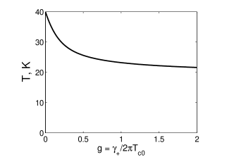
Figure 4: Dependence of the critical temperature $T_{c}$ on the interband scattering parameter g calculated from Eq. (13) with the BCS matrix constants $\lambda_{mn}$ from Ref. goluba

IV Upper critical field for ${\bf H}\|c$

$H_{c2}$ along the c-axis is the maximum eigenvalue of the linearized Eqs. (2) and (3):

$$(\omega\pm i\mu_{B}H)f_{1}-\frac{D_{1}}{2}\Pi^{2}f_{1}=\Delta_{1}+(f_{2}-f_{1})\gamma_{12},$$ (17)

$$(\omega\pm i\mu_{B}H)f_{2}-\frac{D_{2}}{2}\Pi^{2}f_{2}=\Delta_{2}+(f_{1}-f_{2})\gamma_{21},$$ (18)

Here the Zeeman paramagnetic term $\pm\mu_{B}H$, which requires summation over both spin orientations in Eq. (4), is included. In the gauge $A_{y}=Hx$, the solutions are $f_{m}(x)=\tilde{f}_{m}\exp(-\pi Hx^{2}/\phi_{0})$, and $\Delta_{m}(x)=\tilde{\Delta}_{m}\exp(-\pi Hx^{2}/\phi_{0})$, where $\tilde{f}_{m}$ is expressed via $\tilde{\Delta}_{m}$ from Eqs. (17) and (18). The solvability condition (4) of two linear equations for $\tilde{\Delta}_{1}$ and $\tilde{\Delta}_{2}$ gives the equation for $H_{c2}$ ag , which accounts for interband and intraband scattering and paramagnetic effects:

$$(\lambda_{0}+\lambda_{i})(\ln t+U_{+})+(\lambda_{0}-\lambda_{i})(\ln t+U_{-})$$

$$+2w(\ln t+U_{+})(\ln t+U_{-})=0,$$ (19)

where $t=T/T_{c0}$, and

$$\lambda_{i}=[(\omega_{-}+\gamma_{-})\lambda_{-}-2\lambda_{12}\gamma_{21}-2\lambda_{21}\gamma_{12}]/\Omega_{0},$$ (20)

$$2\Omega_{\pm}=\omega_{+}+\gamma_{+}\pm\Omega_{0},\qquad\qquad$$ (21)

$$\Omega_{0}=[(\omega_{-}+\gamma_{-})^{2}+4\gamma_{12}\gamma_{21}]^{1/2},\qquad$$ (22)

$$\omega_{\pm}=(D_{1}\pm D_{2})\pi H/\phi_{0},\qquad\quad$$ (23)

$$U_{\pm}=\mbox{Re}\psi\left(\frac{1}{2}+\frac{\Omega_{\pm}+i\mu_{B}H}{2\pi T}\right)-\psi\left(\frac{1}{2}\right).$$ (24)

If interband scattering and paramagnetic effects are negligible, Eqs. (19)-(24) reduce to a simpler equation ag ; gk , which can be presented in the parametric form:

$$\ln t=-[U(h)+U(\eta h)+\lambda_{0}/w]/2+$$ (25)

$$[(U(h)-U(\eta h)-\lambda_{-}/w)^{2}/4+\lambda_{12}\lambda_{21}/w^{2}]^{1/2},$$

$$H_{c2}=2\phi_{0}T_{c}th/D_{1},\qquad\qquad$$ (26)

where $\eta=D_{2}/D_{1}$, and the parameter h runs from $0$ to $\infty$ as T varies from $T_{c}$ to 0. For equal diffusivities, $\eta=1$, Eq. (IV) simplifies to the one-gap de-Gennes-Maki equation $\ln t+U(h)=0$ dege ; whh ; maki .

Now we consider some limiting cases, which illustrate how $H_{c2}$ depends on different parameters. Fig. 5 shows the evolution of $H_{c2}$ as $g$ increases for fixed $D_{1}$ and $D_{2}$ and negligible paramagnetic effects. Interband scattering reduces the upward curvature of $H_{c2}(T)$, $H_{c2}(0)$, and $T_{c}$, while increasing the slope $H_{c2}^{\prime}$ at $T_{c}$. Notice that the significant changes in the shape of $H_{c2}(T)$ in Fig. 5 occur for weak interband scattering ($g\ll 1$), which also provides a finite $H_{c2}(0)$ even if $D_{2}\to 0$. For example, the high-field films in Fig. 1 and 2 have $g\simeq 0.045$ and $0.065$, respectively. For $g\ll 1$, Eq. (19) yields the GL linear temperature dependence near $T_{c}$:

$$H_{c2}=\frac{8\phi_{0}(T_{c}-T)}{\pi^{2}(s_{1}D_{1}+s_{2}D_{2})}$$ (27)

where $T_{c}$ is given by Eq. (16), $s_{1}=1+\lambda_{-}/\lambda_{0}$ and $s_{2}=1-\lambda_{-}/\lambda_{0}$. Eq. (27) is written in the linear accuracy in $g\ll 1$. Higher order terms in g not only shift $T_{c}$ but also increase the slope $H_{c2}^{\prime}$ at $T_{c}$, as evident from Fig. 5. For $s_{1}\sim s_{2}$, the slope $H_{c2}^{\prime}$ is mostly determined by the cleanest band with the maximum diffusivity. However, because of weak interband coupling in MgB₂, the values of $s_{1}$ and $s_{2}$ are very different. For $\lambda_{11}=0.81$, $\lambda_{22}=0.285$, $\lambda_{12}=0.119$, $\lambda_{21}=0.09$ goluba , we get $\lambda_{-}=\lambda_{11}-\lambda_{22}=0.525$, $\lambda_{0}=(\lambda_{-}^{2}+4\lambda_{12}\lambda_{21})^{1/2}=0.564$, thus $s_{1}=1+\lambda_{-}/\lambda_{0}=1.93$, $s_{2}=1-\lambda_{-}/\lambda_{0}=0.07$. Thus, $H_{c2}^{\prime}$ is mostly determined by $D_{1}$ of the $\sigma$ band. Yet, if the $\sigma$ band is so dirty that $D_{1}/D_{2}<s_{2}/s_{1}\simeq 0.04$, the slope $H_{c2}^{\prime}$ is determined by the much cleaner $\pi$ band.

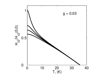
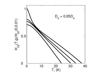
Figure 5: Effect of interband scattering and the diffusivity ratio on the evolution of $H_{c2}(T)$. Upper panel shows $H_{c2}(T,\eta)$ for the fixed $g=0.03$ and different $\eta=D_{2}/D_{1}$: $0;0.05;0.1;0.5$ (from top to bottom curves). Lower panel shows $H_{c2}(T,g)$ for the fixed $D_{2}/D_{1}=0.05$ and different $g=0.01;0.05;0.1;0.5$ (from top to bottom curves).

At low T both the Zeeman and interband scattering terms in Eq. (19) can be essential. Eq. (19) reduces to the following equation for $H_{c2}(0)$:

$$(\lambda_{0}+\lambda_{i})\ln\frac{\mu_{B}^{2}H_{p}^{2}}{\mu_{B}^{2}H^{2}+\Omega_{+}^{2}}+(\lambda_{0}-\lambda_{i})\ln\frac{\mu_{B}^{2}H_{p}^{2}}{\mu_{B}^{2}H^{2}+\Omega_{-}^{2}}$$

$$=w\ln\frac{\mu_{B}^{2}H_{p}^{2}}{\mu_{B}^{2}H^{2}+\Omega_{+}^{2}}\ln\frac{\mu_{B}^{2}H_{p}^{2}}{\mu_{B}^{2}H^{2}+\Omega_{-}^{2}}\qquad\qquad$$ (28)

where $\mu_{B}H_{p}=\pi T_{c0}/2\gamma$ is the field of paramagnetic instability of the superconducting state, and $\ln\gamma=0.577$. We first consider the limit $g\to 0$, which defines the maximum $H_{c2}(0)$ achievable in a dirty two-gap superconductor with no $T_{c}$ suppresion. In this case $\Omega_{+}=\pi D_{1}H/\phi_{0}$ and $\Omega_{-}=\pi D_{2}H/\phi_{0}$, so for $T\ll T_{c}$, paramagnetic effects just renormalize intraband diffusivities in Eq. (28):

$$D_{m}\to\tilde{D}_{m}=\sqrt{D_{m}^{2}+D_{0}^{2}},$$ (29)

where $D_{0}=\mu_{B}\phi_{0}/\pi$ is the quantum diffusivity

$$D_{0}=\hbar/2m,$$ (30)

and $m$ is the bare electron mass. Eq. (30) follows from the basic diffusion relation $l^{2}=D_{0}t$, and the energy uncertainty principle $\hbar^{2}/2ml^{2}=\hbar/t$ for a particle confined in a region of length $l$. For $g=0$, Eq. (28) yields

$$H_{c2}(0)=\frac{\phi_{0}T_{c}}{2\gamma\sqrt{\tilde{D}_{1}\tilde{D}_{2}}}\exp(\frac{f}{2}),\qquad\qquad$$ (31)

$$f=\left(\frac{\lambda_{0}^{2}}{w^{2}}+\ln^{2}\frac{\tilde{D}_{2}}{\tilde{D}_{1}}+\frac{2\lambda_{-}}{w}\ln\frac{\tilde{D}_{2}}{\tilde{D}_{1}}\right)^{1/2}-\frac{\lambda_{0}}{w}.\quad$$ (32)

If $D_{0}\ll D_{m}$, Eqs. (31)-(32) reduce to the result of Ref. ag , and for the symmetric case, $\tilde{D}_{1}=\tilde{D}_{2}$, Eqs. (31)-(32) give the one-band result $H_{c2}(0)=\phi_{0}T_{c}/2\gamma\tilde{D}$ whh . However for $\tilde{D}_{1}\neq\tilde{D}_{2}$, $H_{c2}(0)$ can be much higher than $H_{c2}(0)=0.69H_{c2}^{\prime}T_{c}$. Indeed, if the effective diffusivities, $\tilde{D}_{1}$ and $\tilde{D}_{2}$ are very different, Eqs. (31)-(32) yield

$$H_{c2}(0)=\frac{\phi_{0}T_{c}}{2\gamma\tilde{D}_{2}}e^{-(\lambda_{-}+\lambda_{0})/2w},\qquad\tilde{D}_{2}\ll\tilde{D}_{1}e^{-\frac{\lambda_{0}}{w}},$$ (33)

$$H_{c2}(0)=\frac{\phi_{0}T_{c}}{2\gamma\tilde{D}_{1}}e^{-(\lambda_{0}-\lambda_{-})/2w},\qquad\tilde{D}_{1}\ll\tilde{D}_{2}e^{-\frac{\lambda_{0}}{w}}.$$ (34)

Thus, $H_{c2}(0)$ is determined by the minimum effective diffusivity, but unlike the limit $D_{0}\to 0$, $H_{c2}(0)$ remains finite even for $D_{1}\to 0$ or $D_{2}\to 0$. In fact, if both $D_{1}\ll D_{0}$ and $D_{2}\ll D_{0}$, we return to the symmetric case $\tilde{D}_{1}=\tilde{D}_{2}$, for which Eqs. (31)-(32) yield the result of the one-gap dirty limit theory maki

$$H_{c2}(0)\to H_{p}=\phi_{0}T_{c}/2\gamma D_{0}=\pi T_{c}/2\gamma\mu_{B}$$ (35)

For a one-band superconductor, Eq. (35) can also be written as the paramagnetic pairbreaking condition, $\mu_{B}H_{p}=\Delta(0)/2$, where $\Delta(0)=\pi T_{c}/\gamma$ is the zero-temperature gap. For two-band superconductors, the meaning of $H_{p}$ is less transparent, yet the maximum $H_{p}$ expressed via $T_{c}$ is given by the same Eq. (35) as for one-band superconductors.

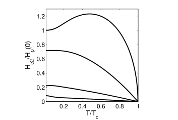
Figure 6: Crossover from the orbitally to paramagnetically limited $H_{c2}(T)$ calculated from Eqs. (IV) and (37)-(38) for $D_{2}=0.05D_{1}$ and $D_{1}/D_{0}=0,1,5,20$ from top to bottom curves, respectively.

Finally we consider how paramagnetic effects affect the shape of $H_{c2}(T)$ in the limit $g\to 0$. This case is described by Eq. (26) modified as follows:

$$U(h)\to\mbox{Re}\psi[1/2+h(i+p)]-\psi(1/2)$$ (36)

$$U(\eta h)\to\mbox{Re}\psi[1/2+h(p\eta+i)]-\psi(1/2)$$ (37)

$$H_{c2}=H_{c2}=2\phi_{0}T_{c}th/D_{0},\qquad\qquad$$ (38)

where $p=D_{1}/D_{0}$, and $\eta=D_{2}/D_{1}$. Fig. 6 shows how $H_{c2}(T)$ evolves from the orbitally-limited $H_{c2}(T)$ with an upward curvature at $D_{1}\gg D_{2}$ to the paramagnetically-limited $H_{c2}(T)$ of a one-gap superconductor for $D_{1}<D_{0}$ par3 . The nonmonotonic dependence of $H_{c2}(T)$ in Fig. 6 indicates the first order phase transition, similar to that in one-gap superconductors.

V Thin films in a parallel field

$H_{c2}$ can be significantly enhanced in thin films or multilayers, in which MgB₂ layers are separated by nonsuperconducting layers. It is well known that in a thin film of thickness $d<\xi$ in a parallel field, $H_{c2}^{(f)}=2\sqrt{3}H_{c2}\xi/d$ can be higher than the bulk $H_{c2}=\phi_{0}/2\pi\xi^{2}$ layer2 ; tink . Let us see how this result is generalized to two-gap superconductors. For a thin film of thickness $d<\mbox{max}(\xi_{1},\xi_{2})$, the functions $f_{1}$ and $f_{2}$ are nearly constant, so integrating Eqs. (17) and (18) over x with $\partial_{x}f(\pm d/2)=0$, results in two linear equations for $f_{1}$ and $f_{2}$ with $\Pi^{2}=(\pi Hd/\phi_{0})^{2}/3$. Thus, we obtain the previous Eq. (19)-(24) in which one should make the replacement

$$\omega_{\pm}^{(f)}\to(\pi Hd/\phi_{0})^{2}(D_{1}\pm D_{2})/6$$ (39)

We first consider the case of negligible interband scattering and paramagnetic effects. Then Eq. (19) and (39) give the square-root temperature dependence near $T_{c}$

$$H_{c2}^{(f)}=\frac{4\phi_{0}\sqrt{3T_{c}(T_{c}-T)}}{\pi^{3/2}d(s_{1}D_{1}+s_{2}D_{2})^{1/2}}$$ (40)

characteristic of thin films tink instead of the bulk GL linear dependence (27). From Eqs. (31) and (39) we can also obtain $H_{c2}^{(f)}(0)$ for $D_{0}\ll D_{m}$:

$$H_{c2}^{(f)}(0)=\frac{\phi_{0}}{d}\left(\frac{3T_{c}}{\pi\gamma}\right)^{1/2}\frac{\exp(f/4)}{(D_{1}D_{2})^{1/4}}$$ (41)

Next we consider the crossover to the paramagnetic limit in thin films at low temperatures. For neglect interband scattering, the expressions $\mu_{B}^{2}H^{2}+\Omega^{2}$ under the logarithms in Eq. (28) become $\mu_{B}^{2}H^{2}+(\pi Hd/\phi_{0})^{4}D^{2}/36$. Substituting here $H_{c2}^{(f)}\sim\phi_{0}/\xi d$, we conclude that paramagnetic effects become essential if

$$\mbox{min}(D_{1},D_{2})<D_{0}\xi/d.$$ (42)

Thus, reducing the film thickness extends the region of the parameters where $H_{c2}$ is limited by the paramagnetic effects rather than by impurity scattering.

VI Anisotropy of $H_{c1}$ and $H_{c2}$

For anisotropic one-gap superconductors, the angular dependence of the lower and the upper critical fields is given by gork ; bul

$$H_{c1}(\alpha,T)=\frac{H_{c1}(0,T)}{R(\alpha)},\quad H_{c2}(\alpha,T)=\frac{H_{c2}(0,T)}{R(\alpha)}$$ (43)

where $R(\alpha)=(\cos^{2}\alpha+\epsilon\sin^{2}\alpha)^{1/2}$, $\epsilon=m_{ab}/m_{c}$. Here the anisotropy parameter $\Gamma(T)=H_{c2}^{||}/H_{c2}^{\perp}={\epsilon}^{-1/2}$ is independent of T for both $H_{c1}$ and $H_{c2}$. By contrast, $\Gamma_{2}(T)=H_{c2}^{||}/H_{c2}^{\perp}$ for MgB₂ single crystals increases from $\sim 2-3$ at $T_{c}$ to $5-6$ at $T\ll T_{c}$, but $\Gamma_{1}(T)=H_{c1}^{||}/H_{c1}^{\perp}$ decreases from $\simeq 2-3$ to $\simeq 1$ as T decreases a1 ; a2 ; a3 ; a4 ; a5 ; a6 ; a7 ; a8 ; a9 ; a10 ; a11 . This behavior was explained by the two-gap theory in the clean limit vgk ; dahm ; lanis1 ; lanis2 .

The dirty limit is more intricate in the sense that $\Gamma(T)$ can either increase or decrease with T, depending on the diffusivity ratio $D_{2}/D_{1}$. However, the physics of this dependence is rather transparent and can be understood using the bilayer toy model as discussed in the Introduction. Indeed, for very different $D_{1}$ and $D_{2}$, both the angular and the temperature dependencies of $H_{c2}(\alpha,T)$ are controlled by cleaner band at high T and by dirtier band at lower T. For instance, if $D_{2}\ll D_{1}$, the high-T part of $H_{c2}(\alpha,T)$ is determined by the anisotropic $\sigma$ band, while the low-T part is determined by the isotropic $\pi$ band. In this case $\Gamma(T)$ decreases as T decreases, as characteristic of dirty MgB₂ films represented in Figs. 1 and 2. If the $\pi$ band is cleaner than the $\sigma$ band, $\Gamma(T)$ increases as T decreases, similar to single crystals.

For the field ${\bf H}$ inclined with respect to the c-axis, the first Landau level eigenfunction no longer satisfies Eqs. (17), (18) and (4). In this case $f_{m}(\omega,{\bf r})$ are to be expanded in full sets of eigenfunctions for all Landau levels, and $H_{c2}$ becomes a root of a matrix equation $\hat{M}(H_{c2})=0$ ag ; gk . As shown in Ref. ag , this matrix equation for $H_{c2}$ greatly simplifies for the moderate anisotropy characteristic of dirty MgB₂ for which all formulas of the previous section can also be used for the inclined field as well by replacing $D_{1}$ and $D_{2}$ with the angular-dependent diffusivities $D_{1}(\alpha)$ and $D_{2}(\alpha)$ for both bands:

$$D_{m}(\alpha)=[D_{m}^{(a)2}\cos^{2}\alpha+D_{m}^{(a)}D_{m}^{(c)}\sin^{2}\alpha]^{1/2}$$ (44)

In terms of the bilayer model shown in Fig. 1, Eq. (44) just means that Eq. (43) should be applied separately for each of the films. For $g=0$, Eqs. (27) and (44) determine the angular dependence of $H_{c2}(\alpha)$ near $T_{c}$, and the London penetration depth $\Lambda_{\alpha\beta}$ is given by ag

$$\Lambda^{-2}_{\alpha\beta}=\frac{4\pi^{4}}{\phi_{0}^{2}}\bigl{[}N_{1}D_{1}^{\alpha\beta}\Delta_{1}\tanh\frac{\Delta_{1}}{2T}+N_{2}D_{2}^{\alpha\beta}\Delta_{2}\tanh\frac{\Delta_{2}}{2T}\bigr{]}$$ (45)

Eqs. (27), (44), and (60) show that the one-gap scaling (43) breaks down because the behavior of $H_{c1}(\alpha,T)$ is mostly controlled by the cleaner band for all T, while the behavior of $H_{c2}(\alpha,T)$ is determined by the cleaner band at higher T, and by the dirtier band at lower T. Thus, $\Gamma_{1}(T)$ and $\Gamma_{2}(T)$ for $H_{c1}$ and $H_{c2}$ in the two-gap dirty limit are different. Temperature dependencies of $\Gamma(T)$ were calculated in Refs. ag ; gk .

Eqs. (44) and (19) describe well both the temperature and the angular dependencies of $H_{c2}(\alpha,T)$ in dirty MgB₂ films h6 ; h9 ; h10 ; h11 . Eq. (44) is valid if the $\sigma$ band is not too anisotropic, and the off-diagonal elements $M_{mn}\sim\zeta^{m+n}$ are negligible provided that $\zeta\ll 1$ ag . Here

$$\zeta=\frac{(\epsilon_{1}-\epsilon_{2})^{2}\sin^{4}\alpha}{[\sqrt{\cos^{2}\alpha+\epsilon_{1}\sin^{2}\alpha}+\sqrt{\cos^{2}\alpha+\epsilon_{2}\sin^{2}\alpha}]^{4}},$$ (46)

$\epsilon_{1}=D_{1}^{(c)}/D_{1}^{(ab)}$ and $\epsilon_{2}=D_{2}^{(c)}/D_{2}^{(ab)}$. For $\epsilon_{2}=1$, the parameter $\zeta(\alpha)<0.45$ for a rather strong anisotropy $\epsilon_{1}<0.04$ and $\alpha=\pi/2$. For a stronger anisotropy, the condition $\zeta(\alpha)\ll 1$ can still hold in a wide range of $\alpha$, except a vicinity of $\alpha\approx\pi/2$. In this case the calculation of $H_{c2}(\alpha,T)$ requires a numerical solution of the matrix equation for $H_{c2}$ gk . However, the Usadel theory can only be applied to dirty MgB₂ samples which, contrary to the assumption of Ref. gk , usually exhibit much weaker anisotropy $(\Gamma_{2}\simeq 1-2)$ than single crystals. Perhaps, strong impurity scattering and admixture of interband scattering reduce the anisotropy of $D_{1}^{(c)}/D_{1}^{(ab)}\simeq 0.2-0.3$ as compared to that of the Fermi velocities $\langle v^{2}_{c}\rangle_{\sigma}/\langle v^{2}_{ab}\rangle_{\sigma}\sim 0.02$ predicted by ab-initio calculations for single crystals anz1 . The moderate anisotropy of $D_{1}$ in dirty MgB₂ makes the scaling rule (44) a very good approximation, as was recently confirmed experimentally h11 .

VII Ginzburg-Landau equations

The two-gap GL equations were obtained both for the dirty limit without interband scattering ag ; golkosh , and for the clean limit zhit . Here we consider the GL dirty limit, focusing on new effects brought by interband scattering. For $\gamma_{mm^{\prime}}=0$, the Usadel equations near $T_{c}$ yield

$$f_{m}=\Psi_{m}/\omega+D_{m\alpha}\Pi^{2}_{\alpha}\Psi/2\omega^{2}-\Psi_{m}|\Psi_{m}|^{2}/2\omega^{3},$$ (47)

where the principal axis of $D_{\alpha\beta}$ are taken along the crystalline axis. For weak interband scattering, the free energy $F=F_{0}+F_{i}$ contains the free energy $F_{0}\{\Psi_{1},\Psi_{2}\}$ for $\gamma_{mm^{\prime}}=0$ and the correction $F_{i}\{\Psi_{1},\Psi_{2}\}$ linear in $\gamma_{mm^{\prime}}$. Here $F_{0}$ does not have first order corrections in $\gamma_{mm^{\prime}}$ if $\Psi_{m}$ satisfies the GL equations, so $F_{i}$ can be calculated by substituting Eq. (47) into Eq. (9) and expanding $g_{m}\approx 1-|f_{m}|^{2}/2-|f_{m}|^{4}/8$:

$$F_{i}=\pi qT\sum_{\omega>0}[|f_{1}-f_{2}|^{2}+(|f_{1}|^{2}-|f_{2}|^{2})^{2}/4],$$ (48)

where $q=(N_{1}\gamma_{12}+N_{2}\gamma_{21})/2$. Combining $F_{i}$ with $F_{0}$ in the dirty limit for $g=0$ ag , we arrive at the GL free energy $\int FdV$ for $g\ll 1$:

$$F=a_{1}|\Psi_{1}|^{2}+c_{1\alpha}|\Pi_{\alpha}\Psi_{1}|^{2}+b_{1}|\Psi_{1}|^{4}/2$$

$$+a_{2}|\Psi_{2}|^{2}+c_{2\alpha}|\Pi_{\alpha}\Psi_{2}|^{2}+b_{2}|\Psi_{2}|^{4}/2$$

$$-a_{i}{\mbox{R}e}(\Psi_{1}\Psi_{2}^{*})+c_{i\alpha}{\mbox{R}e}(\Pi_{\alpha}\Psi_{1}\Pi_{\alpha}^{*}\Psi_{2}^{*})$$

$$-b_{i}|\Psi_{1}|^{2}|\Psi_{2}|^{2}+2b_{i}(|\Psi_{1}|^{2}+|\Psi_{2}|^{2}){\mbox{R}e}(\Psi_{1}\Psi_{2})$$ (49)

Here the GL expansion coefficients are given by

$$a_{1}=\frac{N_{1}}{2}\bigl{[}\ln\frac{T}{T_{1}}+\frac{\pi\gamma_{12}}{4T}\bigr{]},$$ (50)

$$a_{2}=\frac{N_{2}}{2}\bigl{[}\ln\frac{T}{T_{2}}+\frac{\pi\gamma_{21}}{4T}\bigr{]},$$ (51)

$$c_{1\alpha}=N_{1}D_{1\alpha}\bigl{[}\frac{\pi}{16T}-\frac{7\zeta(3)\gamma_{12}}{8\pi^{2}T^{2}}\bigr{]},$$ (52)

$$c_{2\alpha}=N_{2}D_{2\alpha}\bigl{[}\frac{\pi}{16T}-\frac{7\zeta(3)\gamma_{21}}{8\pi^{2}T^{2}}\bigr{]},$$ (53)

$$b_{1}=N_{1}\bigl{[}\frac{7\zeta(3)}{16\pi^{2}T^{2}}-\frac{3\pi\gamma_{12}}{384T^{3}}\bigr{]},$$ (54)

$$b_{2}=N_{2}\bigl{[}\frac{7\zeta(3)}{16\pi^{2}T^{2}}-\frac{3\pi\gamma_{21}}{384T^{3}}\bigr{]},$$ (55)

$$a_{i}=\frac{N_{1}}{2}\bigl{[}\frac{\lambda_{12}}{w}+\frac{\pi\gamma_{12}}{4T}\bigr{]}+\frac{N_{2}}{2}\bigl{[}\frac{\lambda_{21}}{w}+\frac{\pi\gamma_{21}}{4T}\bigr{]},$$ (56)

$$c_{i}=\frac{7\zeta(3)}{(4\pi T)^{2}}(D_{1}+D_{2})(\gamma_{12}N_{1}+\gamma_{21}N_{2}),$$ (57)

$$b_{i}=\frac{\pi}{384T^{3}}(\gamma_{12}N_{1}+\gamma_{21}N_{2}),$$ (58)

where $T_{1}=T_{c0}\exp[-(\lambda_{0}-\lambda_{-})/2w]$, and $T_{2}=T_{c0}\exp[-(\lambda_{0}+\lambda_{-})/2w]$. The GL equations are obtained by varying $\int FdV$. I would like to point out the misprints with wrong signs of $a_{i}$, $c_{1}$ and $c_{2}$ in Eqs. (13), (14) and (20) in Ref. ag (see also Ref. zhit ).

The first two lines in Eq. (49) are the GL intraband free energies and the term $a_{i}{\mbox{R}e}(\Psi_{1}\Psi_{2}^{*})$ describes the Josephson coupling of $\Psi_{1}$ and $\Psi_{2}$. Interband scattering increases $a_{1}$ and $a_{2}$, and the interband coupling constant $a_{i}$. The net result is the reduction of $T_{c}$ determined by the equation $4a_{1}(T_{c})a_{2}(T_{c})=a_{i}^{2}$, which reproduces Eq. (16). Besides the renormalization of $a_{m}$, $b_{m}$ and $c_{m}$, interband scattering produces new terms, which describe the mixed gradient coupling and the nonlinear quatric interaction of $\Psi_{1}$ and $\Psi_{2}$. Similar terms were introduced in the GL theories of heavy fermions heavyferm and borocarbides sigrist , and phenomenological models of $H_{c2}$ in MgB₂ asker . These terms result from interband scattering, so both $c_{i}$ and $b_{i}$ vanish in the clean limit zhit . The mixed gradient terms in Eq. (49) produce interference terms in the current density ${\bf J}=-c\delta F/\delta{\bf A}$:

$${\bf J}=-[(2c_{1}\Delta_{1}^{2}+c_{i}\Delta_{1}\Delta_{2}\cos\theta){\bf Q}_{1}+$$

$$(2c_{2}\Delta_{2}^{2}+c_{i}\Delta_{1}\Delta_{2}\cos\theta){\bf Q}_{2}+$$

$$c_{i}(\Delta_{2}\nabla\Delta_{1}-\Delta_{1}\nabla\Delta_{2})\sin\theta]2\pi c/\phi_{0}$$ (59)

where ${\bf Q}_{m}=\nabla\theta_{m}+2\pi{\bf A}/\phi_{0}$, and $\theta=\theta_{1}-\theta_{2}$. Here ${\bf J}$ is no longer the sum of independent contributions of two bands, because phase gradients in one band produce currents in the other. Moreover, ${\bf J}$ acquires new $\cos\theta$ terms and the peculiar $\sin\theta$ interband Josephson-like contribution for inhomogeneous gaps. For currents well below the depairing limit, both bands are phase-locked ($\theta=0$), and Eq. (59) defines the London penetration depth $\Lambda^{2}=c\phi_{0}Q/8\pi^{2}|J|$:

$$\Lambda=\phi_{0}/4\pi[2\pi(c_{1}\Delta_{1}^{2}+c_{i}\Delta_{1}\Delta_{2}+c_{2}\Delta_{2}^{2})]^{1/2}$$ (60)

where $c_{1}$, $c_{2}$ and $c_{i}$ depend on the field orientation according to Eq. (44). Eq. (47) can be used to calculate $H_{c2}^{\perp}(T)$ from the linearized GL equations, which give $H_{c2}$ as a solution of the quadratic equation sigrist

$$4\left[\frac{2\pi c_{1}H}{\phi_{0}}+a_{1}\right]\left[\frac{2\pi c_{2}H}{\phi_{0}}+a_{2}\right]=\left[a_{i}+\frac{2\pi c_{i}H}{\phi_{0}}\right]^{2}$$ (61)

which reduces to Eq. (27) near $T_{c}$ to the linear accuracy in $\gamma_{mm^{\prime}}$. However, GL calculations of $H_{c2}(T)$ in MgB₂ beyond the linear $T_{c}-T$ term asker ; zhit1 have a rather limited applicability, since $a_{1}(T)$ and $a_{2}(T)$ change signs at very different temperatures $T_{1}$ and $T_{2}$. For $\lambda_{mn}$ of Ref. goluba , $T_{1}\sim 0.9T_{c0}$ and $T_{2}\sim 0.1T_{c0}$ so higher order gradient terms (automatically taken into account in the Eliashberg/Eilenberger/Usadel based theories) become important. For example, at $T\approx T_{1}$ where $a_{2}(T_{1})\gg a_{1}(T)$, retaining the first gradient term $\propto c_{2}$ requires taking into account a next order term $\sim H^{2}$ in the first brackets in Eq. (61), which is beyond the GL accuracy. Thus, applying the GL theory in a wider temperature range asker ; zhit1 makes it a procedure of unclear accuracy, which can result in a spurious upward curvature in $H_{c2}(T)$ not always present in a more consistent theory (for example, in the dirty limit at $D_{1}\simeq D_{2}$). In addition, the anisotropy of $D_{1}(\alpha)$ may further limit the applicability of the GL theory for ${\bf H}||ab$, as for $c_{1}\gg c_{2}$ higher order gradient terms in the $\pi$ band become important golkosh .

VIII Discussion

The remarkable ten-fold increase of $H_{c2}(T)$ in C-doped MgB₂ films h6 ; h7 ; h8 ; h9 ; h10 has brought to focus new and largely unexplored physics and materials science of two-gap superconducting alloys. Moreover, the observations of $H_{c2}$ close to the BCS paramagnetic limit poses the important question of how far can $H_{c2}$ be further increased by alloying. This possibility may be naturally built in the band structure of MgB₂, which provides weak interband coupling and weak interband scattering, thus allowing MgB₂ to be alloyed without strong suppression of $T_{c}$. For example, for the C-doped MgB₂ film shown in Fig. 1, $\rho_{n}$ was increased from $\simeq 0.4\mu\Omega$cm to $560\mu\Omega$cm, yet $T_{c}$ was only reduced down to $35$K h9 . It is the weakness of interband scattering, which apparently makes it possible to take advantage of very dirty $\pi$ band to significantly boost $H_{c2}$ in carbon-doped films which typically have $D_{\pi}\sim 0.1D_{\sigma}$. The reasons why scattering in the $\pi$ band of C-doped MgB₂ films is so much stronger than in the $\sigma$ band has not been completely understood, but another immediate benefit for high-field magnet applications ap1 is that carbon alloying significantly reduces the anisotropy of $H_{c2}$ down to $\Gamma(T)\simeq 1-2$.

Despite many yet unresolved issues concerning the two-gap superconductivity in MgB₂ alloys, $H_{c2}$ of C-doped MgB₂ has already surpassed $H_{c2}$ of Nb₃Sn (see Fig. 1). Given the intrinsic weakness of interband scattering, which enables tuning MgB₂ by selective atomic substitutions on Mg and B sites, there appear to be no fundamental reasons why $H_{c2}$ of MgB₂ alloys cannot be pushed further up toward the strong-coupling paramagnetic limit (1). Thus, understanding the mechanisms of intra and interband impurity scattering in carbon-doped MgB₂, and the competition between scattering and doping effects becomes an important challenge for the computational physics. For instance, it remains unclear why the multiphased C-doped HPCVD grown films penn exhibit higher $H_{c2}$ and weaker $T_{c}$ suppression h9 than uniform carbon solid solutions h7 ; carb1 ; carb2 . This unexpected result may indicate other extrinsic mechanisms of $H_{c2}$ enhancement, which are not accounted by the simple two-gap theory presented here. Among those may be effects of electron localization or strong lattice distortions in multiphased C-doped films which can manifest themselves in the buckling of the Mg planes observed in the dirty fiber-textured MgB₂ films shown in Fig. 2 h6 . Such buckling may enhance scattering in the $\pi$ band formed by out-of-plane $p_{z}$ boron orbitals.

Recently significant enhancements of vortex pinning and critical current densities $J_{c}$ in MgB₂ jc1 ; jc2 ; jc3 ; jc4 ; jc5 ; jc6 ; jc7 has been achieved, particularly by introducing SiC jc3 and ZrB₂ jc6 nanoparticles. Given these promising results combined with weak current blocking by grain boundaries dcl , the lack of electromagnetic granularity mo , and very slow thermally-activated flux creep creep1 ; creep2 , it is not surprising that MgB₂ is being regarded as a strong contender of traditional high-field magnet materials like NbTi and Nb₃Sn. Despite these achievements, a detailed theory of pinning in MgB₂ is trill lacking. Such theory should take into account a composite structure of the vortex core, which consists of concentric regions of radius $\xi_{\sigma}$ and $\xi_{\pi}$ where $\Delta_{\sigma}(r)$ and $\Delta_{\pi}(r)$ are suppressed vort1 ; vort2 ; vort3 ; vort4 ; vort5 ; vort6 . For example, in MgB₂ single crystals the larger vortex cores in the $\pi$ band start overlapping above the ”virtual upper critical field” $H_{v}=\phi_{0}/2\pi\xi_{\pi}^{2}\sim 0.5T$, causing strong overall suppression of $\Delta_{\pi}$ well below $H_{c2}$ vort2 ; vort3 . This effect can reduce $J_{c}$ at $H>H_{v}$, however both $H_{v}$ and $H_{c2}$ can be greatly increased by appropriate enhancement of impurity scattering in MgB₂ alloys.

Recently there has been an emerging interest in microwave response of MgB₂ rf1 ; rf2 ; rf3 and a possibility of using MgB₂ in resonant cavities for particle accelerators rf4 ; rf5 . These issues require understanding nonlinear electrodynamics and current pairbreaking in two-gap superconductors kunchur ; nicol , in particular, band decoupling and the formation of interband phase textures at strong rf currents text1 ; text2 .

This work was partially supported by in-house research program at NHMFL. NHMFL is operated under NSF Grant DMR-0084173 with support from state of Florida.

References

- (1) J. Nagamatsu, N. Nakagawa, T. Muranaka, Y. Zenitani, J. Akimitsu. Nature 410 (2001) 63.
- (2) A. Liu, I.I. Mazin, J. Kortus. Phys. Rev. Lett. 87 (2001) 087005.
- (3) H.J. Choi, D. Roundy, H. Sun, M.L. Cohen, S.G. Loule. Nature 418 (2002) 758; Phys. Rev. B 66 (2002) R020513.
- (4) A. Floris et al. Phys. Rev. Lett. 94 (2005) 037004.
- (5) C. Buzea, T. Yamashita, Supercond. Sci. Technol. 14 (2001) R115.
- (6) P.C. Canfield, S.L. Bud’ko, D.K. Finnemore. Physica C385 (2003) 1.
- (7) H. Suhl, B.T. Matthias, L.R. Walker, Phys. Rev. Lett. 3 (1959) 552.
- (8) V.A. Moskalenko. Fiz. Met. Metalloved. 8 (1959) 503 [Sov. Phys. Met. Metallog. 8 (1959) 25]; V. A. Moskalenko, M.E. Palistrat, V.M. Vakalyuk, Usp. Fiz. Nauk, 161 (1991) 155 [Sov. Phys. Usp. 34 (1991) 717].
- (9) S.V. Shulga, S.-L. Drechsler, G. Fuchs, K.-H. Müller, K. Winzer, M. Heinecke, K. Krug. Phys. Rev. Lett. 80, (1998) 1730; S.V. Shulga et al. cond-mat/0103154.
- (10) V. Guritani, W. Goldacker, F. Bouquet, Y. Wang, R. Lortz, G. Goll, A. Junod, Phys. Rev. B 70, (2004) 184526.
- (11) Y. Yokoya, T. Kiss, A. Chainani, S. Shin, M. Mikara, H. Takagi. Science 294 (2001) 2518; E. Boaknin et al. Phys. Rev. Lett. 90 (2003) 117003.
- (12) G. Seyfarth et al. Phys. Rev. Lett. 95 (2005) 107004.
- (13) J. Singleton, C. Mielke. Contempor. Phys. 43 (2002) 63.
- (14) I.I. Mazin et al. Phys. Rev. Lett. 89 (2002) 107002.
- (15) A.J. Legget. Prog. Theor. Phys. 36 (1966) (901); Rev. Mod. Phys. 47 (1975) 331.
- (16) A. Gurevich, V.M. Vinokur. Phys. Rev. Lett. 90 (2003) 047004.
- (17) A. Gurevich, V.M. Vinokur. Phys. Rev. Lett. 97 (2006) 137003.
- (18) T.P. Orlando, E.J. McNiff, S. Foner, M.R. Beasley. Phys. Rev. B19 (1979) 4545.
- (19) A. Godeke. Supercond. Sci. Technol. 19 (2006) R68.
- (20) S. Patnaik et al. Supercond. Sci. Technol. 14 (2001) 315.
- (21) C.B. Eom, et al. Nature 411 (2001) 558.
- (22) V.Ferrando et al. Phys. Rev. B 68 (2003) 0945171.
- (23) F. Bouquet, et al. Physica C 385, (2003) 192.
- (24) E. Ohmichi, T. Masui, S. Lee, S. Tajima, T. Osada. J. Phys. Soc. Japan, 73 (2004) 2065.
- (25) A. Gurevich et al. Supercond. Sci. Technol. 17 (2004) 278.
- (26) R.T.H. Wilke, S.L. Bud’ko, P.C. Canfield, D.K. Finnemore, R.J. Suplinskas, S.T. Hannahs. Phys. Rev. Lett. 92 (2004) 217003.
- (27) A.V. Pogrebnyakov et al. Appl. Phys. Lett. 85 (2004) 2017.
- (28) V. Braccini et al. Phys. Rev. B 71, (2005) 012504.
- (29) M. Angst, S.L. Budko, R.H.T. Wilke, P.C. Canfield. Phys. Rev. B 71 (2005) 144512.
- (30) H.-J. Kim, H.-S. Lee, B. Kang, W.-H. Yim, Y. Jo, M.-H. Jung, S.-I. Lee. Phys. Rev. B 73 (2006) 064520.
- (31) P. Samuely, P. Szabo, Z. Holanova, S. Budko, P. Canfield. Physica C435 (2006) 71.
- (32) X.X. Xi et al. Supercond. Sci. Technol. 17 (2004) 196.
- (33) A.A. Abrikosov, L.P. Gor’kov. Zh. Exper. Teor. Fiz., 36 (1959) 319.
- (34) P.G. De Gennes. Phys. Cond. Materie 3 (1964) 79.
- (35) E. Helfand, N.R. Werthamer. Phys. Rev. 147 (1966) 288; N.R. Werthamer, E. Helfand, P.C. Hohenberg. Phys. Rev. 147 (1966) 295.
- (36) K. Maki. Phys. Rev. 148 (1966) 362.
- (37) D. Larbalestier, A. Gurevich, D.M. Feldmann, A. Polyanskii. Nature 414 (2001) 368.
- (38) A. Gurevich. Phys. Rev. B 67 (2003) 184515.
- (39) A.A. Golubov, A.E. Koshelev. Phys. Rev. B 68 (2003) 1045031.
- (40) M. Mansor, J.P. Carbotte. Phys. Rev. B72 (2005) 024538.
- (41) This toy model should not be taken too literally, since in real multilayers in the inclined field can depend on the film thickness due to the effect of surfaces on the nucleation of vortices.
- (42) L.P. Gor’kov, T.K. Melik-Barkhudarov. JETP 18 (1964) 1031.
- (43) L.N. Bulaevskii. Zh. Exp. Teor. Fiz. 64 (1973) 2241; 65 (1973) 1278 [JETP 37 (1973) 1133; 38 (1974) 634].
- (44) D.K. Belashchenko, M. van Schilfgaarde, V.P. Antropov. Phys. Rev. B 64 (2001) 092503.
- (45) I.I. Mazin, V.P. Antropov. Physica C 385 (2003) 49.
- (46) S.L. Bud’ko, V.G. Kogan, P.C. Canfield. Phys. Rev. B 64 (2001) 180506.
- (47) S. Lee, H. Mori, T. Masui, Y. Eltsev, A. Yamamoto, S. Tajima. J. Phys. Soc. Jap. 70 (2001) 2255.
- (48) S.L. Bud’ko, P.C. Canfield. Phys. Rev. B 65 (2002) 212501.
- (49) A.K. Pradhan et al. Phys. Rev. B 64 (2001) 212509.
- (50) M. Angst et al. Phys. Rev. B 88 (2002) 167004.
- (51) A.V. Sologubenko, J. Jun, S.M. Kazakov, J. Karpinski, H.R. Ott. Phys. Rev. B 65 (2002) 180505.
- (52) K. Takahashi, T. Atsumi, N. Yamamoto, M. Xu, H. Kitazawa, T. Ishida. Phys. Rev. B 66 (2002) 012501.
- (53) M. Zehetmayer, M. Eisterer, J. Jun, S.M. Kazakov, J. Karpinski, A. Wisniewski, H.W. Weber. Phys. Rev. B 66 (2002) 052505.
- (54) S.L. Bud’ko, P.C. Canfield, V.G. Kogan. Physica C 387 (2002) 85.
- (55) A. Rydh et al. Phys. Rev. B 70 (2004) 132503.
- (56) L. Lyard et al. Phys. Rev. Lett. 92 (2004) 057001.
- (57) V.G. Kogan. Phys. Rev. B 66 (2002) 020509.
- (58) T. Dahm, N. Schopohl. Phys. Rev. Lett. 91 (2003) 017001.
- (59) J. Kortus, O.V. Dolgov, R.K. Kremer, A.A. Golubov. Phys. Rev. Lett. 94 (2005) 027002.
- (60) M. Putti et al. Phys Rev. B 70 (2004) 052509 (2004); B 71 (2005) 144505.
- (61) R.J. Cava, H.W. Zandbergen, K. Inumaru. Physica C 385 (2003) 8.
- (62) R.A. Ribeiro, S.L. Bud’ko, C. Petrovic, P.C. Canfield. Physica C 385 (2003) 16.
- (63) J. Karpinski et al. Supercond. Sci. Technol. 16 (2003) 221.
- (64) J. Kim, R.K. Singh, N. Newman, J.M. Rowell. IEEE Trans. Appl. Supercond 13 (2003) 3238.
- (65) G.K. Perkins et al. Nature, 411 (2001) 561.
- (66) M. Eisterer et al. Supercond. Sci. Technol. 15 (2002) L9.
- (67) Y. Wang et al. J. Phys.: Cond. Matter. 15 (2003) 883.
- (68) R. Gandikota et al. Appl. Phys. Lett. 86 (2005) 012508.
- (69) S. Lee, T. Masui, A. Yamamoto, H. Uchiyama, S. Tajima. Physica C 397 (2003) 7.
- (70) T. Masui, S. Lee, S. Tajima. Phys. Rev. B 70, 0245041 (2004).
- (71) T. Kakeshita, S. Lee, S. Tajima. Phys. Rev. Lett. 97 (2006) 037002.
- (72) G. Sarma. J. Phys. Chem. Solids 24 (1963) 1029.
- (73) M. Schossmann, J.P. Carbotte. Phys. Rev. B 39 (1989) 4210.
- (74) H.J. Nui, D.P. Hampshire. Phys. Rev. Lett. 91 (2003) 027002.
- (75) R.A. Klemm, A. Luther, M.R. Beasley. Phys. Rev. B 12 (1975) 877.
- (76) S. Takachashi, M. Tachiki. Phys. Rev. B 33 (1968) 4620.
- (77) A.A. Golubov et al. J. Phys: Condens. Matt. 14 (2002) 1353.
- (78) of Ref. text2 should be multiplied by .
- (79) N. Schophol, K. Scharnberg. Solid State Comm. 22 (1977) 371.
- (80) A.A. Golubov, I.I. Mazin. Phys. Rev. B 55 (1997) 15146.
- (81) M. Iavarone et al. Phys. Rev. B 71 (2005) 214502.
- (82) M. Tinkham. Phys. Rev. B 129 (1963) 2413.
- (83) V.G. Kogan. Phys. Rev. B 66 (2002) R020509; V.G. Kogan, N. Zhelezina. Phys. Rev. B 69 (2004) 1235061.
- (84) A.A. Golubov, A. Brinkman, O.V. Dolgov, J. Kortus, O. Jepsen. Phys. Rev. B 66 (2002) 054524.
- (85) A.A. Golubov, A.E. Koshelev. Phys. Rev. Lett. 68 (2003) 104503.
- (86) M.E. Zhitomirsky, V.H. Dao. Phys. Rev. B 69 (2004) 054508.
- (87) I.N. Askerzade, A. Gencer, N. Güclú. Supercond. Sci. Technol. 15 (2002) L13; I.N. Askerzade. Physica C 390 (2003) 281.
- (88) V.H. Dao, M.E. Zhitomirsky. Eur. J. Phys. 44 (2005) 183.
- (89) H. Doh, M. Sigrist, B.K. Cho, S.-I. Lee. Phys. Rev. Lett. 83 (1999) 5350.
- (90) A. Gümbel, J. Eckert, G. Fuchs, K. Nenkov, K.H. Müller, L. Schultz, Appl. Phys. Lett. 80 (2002) 2725.
- (91) K. Komori et al. Appl. Phys. Lett. 81 (2002) 1047.
- (92) S.X. Dou et al. Appl. Phys. Lett. 81 (2002) 3419.
- (93) J. Wang et al. Appl. Phys. Lett. 81 (2002) 2026.
- (94) R. Flukiger, H.L. Suo, N. Musolino, C. Beneduce, P. Toulemonde, P. Lezza. Physica C 385 (2003) 286.
- (95) M. Bhatia, M.D. Sumption, E.W. Collings, S. Dregia. Appl. Phys. Lett. 87 (2005) 042505.
- (96) B.J. Senkowicz, J.E. Giencke, S. Patnaik, S.B. Eom, E.E. Hellstrom, D.C. Larbalestier. Appl. Phys. Lett. 86 (2005) 202502.
- (97) D.C. Larbalestier et al. Nature 410 (2001) 186.
- (98) A.A. Polyanskii et al. Supercond. Sci. Technol. 14 (2001) 811.
- (99) J.R. Thompson, M. Paranthaman, D.K. Christen, K.G. Sorge, J.G. Ossandon. Supercond. Sci. Technol. 14 (2001) L17.
- (100) S. Patnaik, A. Gurevich, S.D. Bu, J. Choi, C.B. Eom, D.C. Larbalestier. Phys. Rev. B 70 (2004) 064503.
- (101) E. Babaev. Phys. Rev. Lett. 89 (2002) 0670011.
- (102) M.R. Eskildsen et al. Phys. Rev. Lett. 89,187004-4 (2002).
- (103) S. Serventi et al. Phys. Rev. Lett. 93 (2004) 217003.
- (104) A.E. Koshelev, A.A. Golubov. Phys. Rev. Lett. 90 (2003) 177002.
- (105) M. Ichioka, K. Machida, N. Nakai, P. Miranovic. Phys. Rev. B 70 (2004) 1445081.
- (106) A. Guman, S. Graser, T. Dahm, N. Schopohl. Phys. Rev. B 73 (2006) 104506.
- (107) A.T. Findikoglu et al. Phys. Lett. 83 (2003) 108.
- (108) B.B. Jin et al. Appl. Phys. Lett. 87 (2005) 092503.
- (109) G. Cifaiello et al. Appl. Phys. Lett. 88 (2006) 142510.
- (110) E.W. Collings, M.D. Sumption, T. Tajima. Supercond. Sci. Technol. 17 (2004) 595.
- (111) A. Gurevich. Appl. Phys. Lett. 88 (2006) 12511.
- (112) M.N. Kunchur. J. Phys. Cond. Mat. 16 (2004) R1183.
- (113) E.J. Nicol, J.P. Carbotte, D.J. Scalapino. Phys. Rev. B 73 (2006) 014521.