Transport and Helfand moments in the Lennard-Jones fluid. II. Thermal conductivity

Abstract

The thermal conductivity is calculated with the Helfand-moment method in the Lennard-Jones fluid near the triple point. The Helfand moment of thermal conductivity is here derived for molecular dynamics with periodic boundary conditions. Thermal conductivity is given by a generalized Einstein relation with this Helfand moment. We compute thermal conductivity by this new method and compare it with our own values obtained by the standard Green-Kubo method. The agreement is excellent.

I Introduction

This paper completes the analysis carried out in the companion paper Viscardy et al. by the study of thermal conductivity with the Helfand-moment method Helfand (1960). Since the seventies, several works have been carried out for the calculation of the transport coefficients. Shear viscosity is the most studied transport property, while thermal conductivity has been less studied. The first computation of thermal conductivity goes back to the work of Alder et al. for hard-sphere systems Alder et al. (1970). Soft-sphere potential systems were considered for the first time a few years later by Levesque et al. Levesque et al. (1973) using the well-known Green-Kubo formula Green (1951, 1960); Kubo (1957); Mori (1958). Nevertheless, since the autocorrelation function of the microscopic flux decreases slowly, especially near the triple point, most of the studies devoted to the computation of thermal conductivity were performed by nonequilibrium methods. This is usually done by fixing the temperature gradient and measuring the heat flux Ashurst ; Evans (1982); Ciccotti and Tenenbaum (1980); Massobrio and Ciccotti (1984); Evans (1986); Heyes (1988), except in Ref. M ller-Plathe (1997) where the opposite is done, i.e., the heat flux is fixed and the temperature gradient is measured. However, some equilibrium molecular dynamics studies using the standard Green-kubo formula were carried out Levesque et al. (1973); Massobrio and Ciccotti (1984); Heyes (1988); Hoheisel (1990). More recently, as suggested in the nineties Allen (1993); Haile (1997), the generalized Einstein relation expressing thermal conductivity as the variance of the time integral of the microscopic flux was computed Meier (2002). The purpose of the present paper is to extend the Helfand-moment method of the companion paper Viscardy et al. from viscosity to thermal conductivity. As an application of our method, we calculate the thermal conductivity of the Lennard-Jones fluid at a phase point near the triple point. We show that the values obtained by the Helfand-moment method and the Green-Kubo values are in excellent agreement. Such a method brings not only some interest as an alternative equilibrium molecular dynamics method, but also in the context of recent theories in nonequilibrium statistical mechanics. Indeed, the escape-rate formalism propose clear and direct relationships between the transport coefficients and quantities characterizing the microscopic chaos such as the Lyapunov exponents and fractal dimensions Dorfman and Gaspard (1995); Gaspard and Dorfman (1995); Gaspard (1998); Dorfman (1999). Successful results have already been obtained for simple systems: diffusion in the Lorentz gas Gaspard and Baras (1995) and viscosity in a two-particle system Viscardy and Gaspard (2003). Furthermore, the hydrodynamic-mode method, aiming to construct at the microscopic level the hydrodynamic modes which are the solutions of the diffusion or Navier-Stokes equations also depend on the possibility to define Helfand moments in periodic systems. This construction has already been carried out for diffusion in the Lorentz gas Gaspard (1996). By defining the Helfand moment, we hopefully project to extend this construction to the other transport processes, in particular thermal conductivity. The paper is organized as follows. In Section II, the theoretical results of Helfand Helfand (1960) are briefly outlined. In Section III, we present our Helfand-moment method for the calculation of thermal conductivity. Section IV gives the results of the molecular dynamics simulations. We compare our results by the Heldand-moment and Green-Kubo techniques and also to the litterature. Finally, conclusions are drawn in Section V.

II Theoretical background

In the fifties, the Boltzmann and Enskog theories of transport processes were completed by an alternative approach developed by Green Green (1951, 1960), Kubo Kubo (1957) and Mori Mori (1958). This new approach relates the transport coefficients to the time autocorrelation functions of their corresponding microscopic flux. In particular, the thermal conductivity coefficient $\kappa$ can be expressed as

$$\kappa=\lim_{N,V\to\infty}\frac{1}{k_{\rm B}T^{2}V}\int_{0}^{\infty}\left\langle J^{(\kappa)}(0)J^{(\kappa)}(t)\right\rangle\;dt\,.$$ (1)

where $J^{(\kappa)}$ is the microscopic flux associated with thermal conductivity. This theory plays an important role in numerical simulations. On the other hand, Helfand aimed to express the transport coefficients in terms of generalized Einstein relations Helfand (1960) and showed that thermal conductivity is given by

$$\kappa=\lim_{N,V,t\to\infty}\frac{1}{2k_{\rm B}T^{2}Vt}\left\langle\left[G^{(\kappa)}(t)-G^{(\kappa)}(0)\right]^{2}\right\rangle,$$ (2)

where $G^{(\kappa)}(t)$ is the corresponding Helfand moment defined as the centroid

$$G^{(\kappa)}(t)=\sum_{a=1}^{N}x_{a}\left(E_{a}-\left\langle E_{a}\right\rangle\right)\,,$$ (3)

of the energies of the particles

$$E_{a}\equiv\frac{{\bf p}_{a}^{2}}{2m}+\frac{1}{2}\sum_{b(\neq a)}u({\bf r}_{ab})\,.$$ (4)

It can be proved that the Green-Kubo formula (1) and the Helfand equation (2) are equivalent if the microscopic flux is related to the Helfand moment by

$$J^{(\kappa)}(t)=\frac{dG^{(\kappa)}(t)}{dt}\;.$$ (5)

Thanks to Eq. (2), the thermal conductivity coefficient is manifestly a non-negative quantity, as required by the second law of thermodynamics.

III Helfand-moment method

Since the transport coefficients are bulk properties, they can be calculated with equilibrium molecular dynamics with periodic boundary conditions. This dynamics is ruled by Newton’s equations modified in order to take into account the periodicity:

$$\frac{d{\bf r}_{a}}{dt} = \frac{{\bf p}_{a}}{m}+\sum_{s}\Delta{\bf r}_{a}^{(s)}\;\delta(t-t_{s})\;,$$

$$\frac{d{\bf p}_{a}}{dt} = \sum_{b(\neq a)}{\bf F}({\bf r}_{ab})\;;\qquad{\bf F}({\bf r})=-\frac{\partial u({\bf r})}{\partial{\bf r}}\;,$$ (6)

where $\Delta{\bf r}_{a}^{(s)}$ is the jump of the particle $a$ at time $t_{s}$ with $\|\Delta{\bf r}_{a}^{(s)}\|=L$ equal to the length $L$ of the simulation box. The force ${\bf F}({\bf r})$ is here assumed of finite range $r<L/2$. The relative position appearing in the force is defined as

$${\bf r}_{ab}={\bf r}_{a}-{\bf r}_{b}-{\bf L}_{a|b}$$ (7)

where the time-dependent cell translation vector ${\bf L}_{a|b}$ Haile (1997) is chosen for the minimum-image convention $\|{\bf r}_{ab}\|<L/2$ to be satisfied. For more details, see Section III of the companion paper Viscardy et al. . We propose here a Helfand-moment method for thermal conductivity in systems with periodic boundary conditions. As for shear viscosity Viscardy et al. , Helfand’s original expression (3) must be modified in order to take into account the periodicity of the system by the addition of extra terms:

$$G^{(\kappa)}(t)=\sum_{a=1}^{N}x_{a}\left(E_{a}-\left\langle E_{a}\right\rangle\right)+I(t)\,.$$ (8)

Following a way similar to the case of viscosity, we conclude that the Helfand moment which should be used in periodic systems is given by

$$G^{(\kappa)}(t) = \sum_{a}x_{a}\left(E_{a}-\left\langle E_{a}\right\rangle\right)$$ (9)

$$- \sum_{a}\sum_{s}\Delta x_{a}^{(s)}\left(E_{a}-\left\langle E_{a}\right\rangle\right)\theta(t-t_{s})$$

$$- \frac{1}{4}\sum_{a\neq b}\int_{0}^{t}d\tau\;L_{b|ax}\frac{{\bf p}_{a}+{\bf p}_{b}}{m}\cdot{\bf F}({\bf r}_{ab})\,.$$

The derivation is given in Appendix A. As for shear viscosity, the first extra term is due to the jumps of particles from a boundary to the opposite one. The second extra term takes into account of interactions of particles with the image of other particles. By adding the two extra terms to the original Helfand moment, we recover the relation $G=\int dtJ$.

IV Numerical results

We carried out molecular dynamics simulation to apply our Helfand-moment method to the calculation of thermal conductivity in a fluid with the standard 6-12 Lennard-Jones potential $u(r)=4\epsilon\left[(\sigma/r)^{12}-(\sigma/r)^{6}\right]$. All calculations we performed are done with the cutoff $r_{c}=2.5\sigma$. In the reduced units with the time $t^{*}=t\sqrt{\epsilon/(m\sigma^{2})}$ and the space $r^{*}=r/\sigma$, the reduced thermal conductivity is given by

$$\kappa^{*}=\kappa\,\frac{\sigma^{2}}{k_{\rm B}}\sqrt{\frac{m}{\epsilon}}\,.$$ (10)

The details of the simulations are given in the preceding paper Viscardy et al. . To show the validity of the Helfand-moment method, we first compare with the results of the Green-Kubo formula. We depict in Fig. 1 the time derivative of the mean-square displacement of the Helfand moment (3) and the time integral of the autocorrelation function of the microscopic flux. The calculation is carried out for $N=1372$ atoms at the phase point near of the triple point with a reduced temperature of $T^{*}=k_{\rm B}T/\epsilon=0.722$ and a density $n^{*}=n\sigma^{3}=0.8442$. As seen in Fig. 1, the two methods are in perfect agreement.

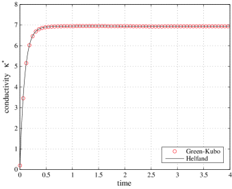
Figure 1: Thermal conductivity at the phase point $T^{*}=0.722$ and $n^{*}=0.8442$ for $N=1372$. The plain line is the derivative of the mean-square displacement of the Helfand moment and the circles the integral of the microscopic flux autocorrelation function.

We estimated thermal conductivity by a linear fit on the mean-square displacement of the Helfand moment. The fit is done in the region between 2 and 8 time units to guarantee that the linear regime is reached. We calculated the thermal conductivity for increasing system sizes from $N=108$ atoms to $N=1372$. We give the results in Table 1 and depict them in Fig. 2 as a function of the inverse $N^{-1}$ of the system size. The linear extrapolation gives the following estimate of thermal conductivity for an infinite system,

$$\kappa^{*}=6.990\pm 0.030\;.$$ (11)

We see in Table 1 that the values of the present work compare very well with the values of previous studies.

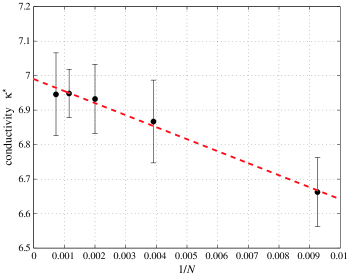
Figure 2: Thermal conductivity at the phase point $T^{*}=0.722$ and $n^{*}=0.8442$ as a function of the inverse of the number $N$ of atoms. The circles are the results of the numerical simulations and the dashed line the linear extrapolation.

Authors	year	method	$r^{*}_{\rm cut}$	$T^{*}$	$N$	$\kappa^{*}$	$\Delta\kappa^{*}$
Levesque et al. Levesque et al. (1973)	1973	GK	N. C.	0.715	256	7.067	0.416
				0.722	864	7.136	0.277
Evans Evans (1982)	1982	EM	2.5	0.722	108	6.54	N. C.
Massobrio and Ciccotti Massobrio and Ciccotti (1984)	1984	GK	3.5	0.721	256	6.880	0.485
		DM	3.5	0.721	256	6.873	0.229
Paolini et al. Paolini et al. (1986)	1986	NEM	2.5	0.718-0.721	averagea)	6.776	0.166
Heyes Heyes (1988)	1988	GK	N. C.	0.72	108	6.7	0.34 ($5\%$)
					256	6.9	0.35 ($5\%$)
					500	6.5	0.33 ($5\%$)
This work	2007	HM (MD)	2.5	0.722	108	6.663	0.10
					256	6.867	0.12
					500	6.932	0.10
					864	6.948	0.07
					1372	6.946	0.12
					$\infty$	6.990	0.061

Table 1: Results found in the literature for the thermal conductivity in the Lennard-Jones fluid near the triple point. The reduced density is $n^{*}=0.8442$ except for Heyes Heyes (1988) ($n^{*}=0.848)$. Abbreviations: DM, nonequilibrium results obtained by the differential method. EM, Evans method Evans (1982). GK, Green-Kubo formula with equilibrium molecular dynamics. NEM, results by nonequilibrium method obtained by Paolini, Ciccotti and Massobrio Paolini et al. (1986). HM, the present Helfand-moment method with molecular dynamics (MD). N. C. means the value has not been communicated.
^a) Thermal conductivity obtained by averaging the values for $N=108,256,500,864$.

V Conclusions

In this paper, a new method is proposed for the calculation of the thermal conductivity in soft-sphere systems. The technique we call the Helfand-moment method is based on generalized Einstein relations (2) with the Helfand moment defined to take into account periodic boundary conditions in the molecular dynamics. This allows us to calculate the thermal conductivity coefficient in terms of the variance of the Helfand moment (9). We show that the original Helfand moment (3) must be modified by adding two extra terms. After the addition of these extra terms, we recover the relation $J=\dot{G}$ between the microscopic flux $J$ and the corresponding Helfand moment $G$. This is the generalization of the case of diffusion for which the velocity $v_{x}$ (the microscopic flux) is related to the position $x$ (the Helfand moment) in the same way $v_{x}=\dot{x}$. Consequently, we have showed that it is possible to calculate the thermal conductivity coefficient by the mean-square displacement of the Helfand moment. Indeed, our molecular dynamics simulations show perfect agreement between the Helfand-moment and Green-Kubo methods. We think that the new expressions for the Helfand moment given in the present and the companion papers Viscardy et al. solve the problems on the use of generalized Einstein relations in periodic systems. In addition to the viscosities Viscardy et al. and thermal conductivity, it is possible to use a similar method for the electric conductivity $\sigma$ in periodic systems. Indeed, by a similar derivation to the one found in Appendix A, one can show that the electric conductivity can be written as:

$$\sigma=\lim_{N,V,t\to\infty}\frac{1}{2k_{\rm B}TVt}\left\langle\left[G^{(\sigma)}(t)-\langle G^{(\sigma)}(t)\rangle\right]^{2}\right\rangle,$$ (12)

where the modified Helfand moment for periodic systems is expressed as:

$$G^{(\sigma)}(t)=\sum_{a}eZ_{a}\left[x_{a}-\sum_{s}\Delta x_{a}^{(s)}\theta(t-t_{s})\right],$$ (13)

with the electric charge $eZ_{a}$ of the particles and $G^{(\sigma)}(0)=0$. Finally, we notice that the Helfand-moment method plays an important role in the escape-rate formalism Dorfman and Gaspard (1995); Gaspard and Dorfman (1995) and the hydrodynamic-mode method Gaspard (1996) developed in nonequibrium statistical mechanics Gaspard (1998). They establish relationships between microscopic and macroscopic levels in the context of the understanding of the origin of the irreversibility of chemical-physical phenomena. The derivation of the Helfand-moment methods give one the possibility to confirm numerically the theoretical predictions of these formalisms.

Appendix A Derivation of the Helfand moment for the thermal conductivity in periodic systems

The time derivative of the modified Helfand moment (8) is given by

$$\frac{dG^{(\kappa)}(t)}{dt} = \sum_{a}\frac{dx_{a}}{dt}\left(E_{a}-\left\langle E_{a}\right\rangle\right)$$ (14)

$$+ \sum_{a}x_{a}\frac{dE_{a}}{dt}+\frac{dI(t)}{dt}$$

where the time derivative of $E_{a}$ is

$$\frac{dE_{a}}{dt} = \frac{{\bf p}_{a}}{m}\cdot\frac{d{\bf p}_{a}}{dt}+\frac{1}{2}\sum_{b(\neq a)}\frac{\partial u_{ab}}{\partial{\bf r}_{ab}}\cdot\frac{{\bf p}_{a}-{\bf p}_{b}}{m}$$ (15)

$$= \frac{1}{2}\sum_{b(\neq a)}\frac{{\bf p}_{a}+{\bf p}_{b}}{m}\cdot{\bf F}({\bf r}_{ab})\;.$$

We notice that there is here no jump in position to consider because $\frac{d{\bf r}_{ab}}{dt}$ concerns a relative position ${\bf r}_{ab}={\bf r}_{a}-{\bf r}_{b}-{\bf L}_{b|a}$ which satisfies the minimum image convention within the range of the force. Symmetrizing the second term in Eq. (14), we find

$$\sum_{a}x_{a}\frac{dE_{a}}{dt} = \frac{1}{4}\sum_{a\neq b}x_{a}\frac{{\bf p}_{a}+{\bf p}_{b}}{m}\cdot{\bf F}({\bf r}_{ab})$$ (16)

$$+ \frac{1}{4}\sum_{a\neq b}x_{b}\frac{{\bf p}_{a}+{\bf p}_{b}}{m}\cdot{\bf F}({\bf r}_{ba})$$

$$= \frac{1}{4}\sum_{a\neq b}x_{ab}\frac{{\bf p}_{a}+{\bf p}_{b}}{m}\cdot{\bf F}({\bf r}_{ab})$$

$$+ \frac{1}{4}\sum_{a\neq b}L_{b|ax}\frac{{\bf p}_{a}+{\bf p}_{b}}{m}\cdot{\bf F}({\bf r}_{ab})$$

where ${\bf F}({\bf r}_{ab})=-{\bf F}({\bf r}_{ba})$ according to Newton’s third law and because $x_{ab}=x_{a}-x_{b}-L_{b|ax}$. Substituting this expression in Eq. (14), where $\frac{dx_{a}}{dt}$ is given by modified Newton’s equations of motion (6), we get the expression

$$\frac{dG^{(\kappa)}(t)}{dt} = \sum_{a}\frac{p_{ax}}{m}\left(E_{a}-\left\langle E_{a}\right\rangle\right)$$ (17)

$$+ \sum_{a}\sum_{s}\Delta x_{a}^{(s)}\left(E_{a}-\left\langle E_{a}\right\rangle\right)\delta(t-t_{s})$$

$$+ \frac{1}{4}\sum_{a\neq b}x_{ab}\frac{{\bf p}_{a}+{\bf p}_{b}}{m}\cdot{\bf F}({\bf r}_{ab})$$

$$+ \frac{1}{4}\sum_{a\neq b}L_{b|ax}\frac{{\bf p}_{a}+{\bf p}_{b}}{m}\cdot{\bf F}({\bf r}_{ab})$$

$$+ \frac{dI(t)}{dt}\;.$$

On the other hand, it is well known that the microscopic flux $J^{(\kappa)}$ for thermal conductivity is given by

$$J^{(\kappa)}(t) = \sum_{a}\frac{p_{ax}}{m}\left(E_{a}-\left\langle E_{a}\right\rangle\right)$$ (18)

$$+ \frac{1}{4}\sum_{a\neq b}x_{ab}\frac{{\bf p}_{a}+{\bf p}_{b}}{m}\cdot{\bf F}({\bf r}_{ab})\;.$$

Since $\frac{dG^{(\kappa)}(t)}{dt}=J^{(\kappa)}(t)$ by definition, we thus obtain that:

$$\frac{dI(t)}{dt} = -\sum_{a}\sum_{s}\Delta x_{a}^{(s)}\left(E_{a}-\left\langle E_{a}\right\rangle\right)\delta(t-t_{s})$$ (19)

$$- \frac{1}{4}\sum_{a\neq b}L_{b|ax}\frac{{\bf p}_{a}+{\bf p}_{b}}{m}\cdot{\bf F}({\bf r}_{ab})\;.$$

Finally, the quantity to be added to the usual Helfand moment (3) is:

$$I(t) = -\sum_{a}\sum_{s}\Delta x_{a}^{(s)}\left(E_{a}-\left\langle E_{a}\right\rangle\right)\theta(t-t_{s})$$ (20)

$$- \frac{1}{4}\sum_{a\neq b}\int_{0}^{t}d\tau\;L_{b|ax}\frac{{\bf p}_{a}+{\bf p}_{b}}{m}\cdot{\bf F}({\bf r}_{ab})\;.$$

References

- (1) S. Viscardy, J. Servantie, and P. Gaspard, companion paper to appear (2007).
- Helfand (1960) E. Helfand, Phys. Rev. 119, 1 (1960).
- Alder et al. (1970) B. J. Alder, D. M. Gass, and T. E. Wainwright, J. Chem. Phys. 53, 3813 (1970).
- Levesque et al. (1973) D. Levesque, L. Verlet, and J. Kürkijarvi, Phys. Rev. A 7, 1690 (1973).
- Green (1951) M. S. Green, J. Chem. Phys. 19, 1036 (1951).
- Green (1960) M. S. Green, Phys. Rev. 119, 829 (1960).
- Kubo (1957) R. Kubo, J. Phys. Soc. Jpn. 12, 570 (1957).
- Mori (1958) H. Mori, Phys. Rev. 112, 1829 (1958).
- (9) W. T. Ashurst, paper presented at the 13th International Conference on Thermal Conductivity, Lake Orzak, Missouri, Nov 5-7, 1973, in Advances in Thermal Conductivity (University of Missouri-Rolla, Rolla, Missouri, 1976), p. 89.
- Evans (1982) D. Evans, Phys. Lett. A 91, 457 (1982).
- Ciccotti and Tenenbaum (1980) G. Ciccotti and A. Tenenbaum, J. Stat. Phys. 23, 767 (1980).