Transport and Helfand moments in the Lennard-Jones fluid. I. Shear viscosity

Abstract

We propose a new method, the Helfand-moment method, to compute the shear viscosity by equilibrium molecular dynamics in periodic systems. In this method, the shear viscosity is written as an Einstein-like relation in terms of the variance of the so-called Helfand moment. This quantity, is modified in order to satisfy systems with periodic boundary conditions usually considered in molecular dynamics. We calculate the shear viscosity in the Lennard-Jones fluid near the triple point thanks to this new technique. We show that the results of the Helfand-moment method are in excellent agreement with the results of the standard Green-Kubo method.

I Introduction

Since Maxwell’s first paper Maxwell (1860); Viscardy on the kinetic theory of gases, shear viscosity as well as the other transport properties are known to find their origin in the microscopic motion of atoms and molecules composing matter. However, it is only since the fifties that exact formulas are known to calculate the transport coefficients in terms of the microscopic dynamics. These so-called Green-Kubo formulas give each transport coefficient as the time integral of the autocorrelation function of some specific microscopic flux associated with the transport property of interest Green (1951, 1960); Kubo (1957); Mori (1958) . Today, the Green-Kubo technique allows us to calculate numerically the transport coefficients by simulating the molecular dynamics of systems with a finite number of particles and periodic boundary conditions.

On the other hand, Einstein classic work on Brownian motion showed that transport properties such as diffusion can also be understood in terms of random walks. It was Helfand Helfand (1960) who identified in 1960 the fluctuating quantities which, by their random walk, are associated with each transport coefficients. These fluctuating quantities are the so-called Helfand moments and are the centroids of the conserved quantity which is transported. In principle, each transport coefficient can thus be obtained from the linear increase of the statistical variance of the corresponding Helfand moment by the so-called generalized Einstein relations. Nevertheless, it is not yet known today how these Helfand moments should be defined in molecular dynamics with periodic boundary conditions, which limits their use in numerical simulations.

The purpose of the present paper is to derive an analytical expression of the Helfand moment associated with viscosity for molecular dynamics with periodic boundary conditions, and to apply the Helfand-moment method to the calculation of shear viscosity in the Lennard-Jones fluid near the triple point.

Already in the first numerical calculation of viscosity in 1970 Alder et al. (1970), the algorithm of Alder et al. was based on generalized Einstein relations derived from the Green-Kubo formulas. The application of the pure Green-Kubo technique by equilibrium molecular dynamics to the Lennard-Jones fluid has been performed a short time after by Levesque et al Levesque et al. (1973) and later by Schoen and Hoheisel Schoen and hoheisel (1985). However, until the middle of the eighties and the work of Schoen and Hoheisel Schoen and hoheisel (1985), as well as the one of Erpenpeck using the Monte-Carlo Metropolis method Erpenbeck (1988), nonequilibrium molecular dynamics was predominantly used for the computation of shear viscosity Lees and Edwards (1972); Ashurst and Hoover (1973); Hoover et al. (1980); Evans (1981); Trozzi and Ciccotti (1984).

At the end of the eighties and the beginning of the nineties, the generalized Einstein relations started to be used for calculating the transport coefficients. An alternative equilibrium molecular dynamics method has been proposed in which the variance of the time integral of the microscopic flux is calculated Allen (1993); Haile (1997). Actually it is the analog of the method of Alder et al.’s Alder et al. (1970) for soft sphere potential systems. Recently, this technique has been applied by Meier et al. Meier et al. (2004), and by Hess and Evans Hess and Evans (2001), the latter having rather considered an equilibrium ensemble of time averages of the flux. In this context, two important points were discussed. The first concerns the so-called McQuarrie expression. In his book McQuarrie (2000), McQuarrie presented Helfand’s formula for the shear viscosity, but with a slightly different form. This difference implied a simplification of the expression, apparently giving an important advantage compared to the original formula Chialvo and Debenedetti (1991); Chialvo et al. (1993); Allen et al. (1994); Allen (1994). The second point concerned the validity of the generalized Einstein relations in periodic systems Haile (1997); Allen (1993); Allen et al. (1994); Erpenbeck (1995). Arguing that the periodic boundary conditions imply that the variance of the original expression of the Helfand moment is bounded in time, the generalized Einstein relations were considered to be impractical in periodic systems. In this paper, we will show that a generalized Einstein relation is available for viscosity after the addition of two terms to the original Helfand moment to take into account the periodicity of the system. The Helfand-moment method presents the important advantage to define shear viscosity as a non-negative quantity, satisfying the positivity of the entropy production. We have previously applied such a method to a system of two hard disks with periodic boundary conditions Viscardy and Gaspard (2003a). In the present paper, we calculate the shear viscosity in a Lennard-Jones fluid near the triple point. We compare the results obtained by the Helfand-moment method with our own Green-Kubo values and those found in the literature.

In addition, the Helfand-moment method plays an important role in the escape-rate formalism. This formalism establishes direct relationships between the characteristic quantities of the microscopic chaos (Lyapunov exponents and fractal dimensions) and the transport coefficients Dorfman and Gaspard (1995); Gaspard and Dorfman (1995); Gaspard (1998); Dorfman (1999). A few years ago, such a relation has been studied for the viscosity in the two-hard-disk model Viscardy and Gaspard (2003b). Furthermore with the use of the Helfand moment, it should be possible to construct at the microscopic level the hydrodynamic modes, which are the solutions of the Navier-Stokes equations. This approach called the hydrodynamic-mode method has been successfully applied for diffusion Gaspard (1996).

The paper is organized as follows. In Section II, we outline the theoretical background of the generalized Einstein formula. Section III is devoted to the presentation of our Helfand-moment method used for the calculation of the shear viscosity in this paper. In Section IV, we discuss the so-called McQuarrie expression and the validity of the generalized Einstein formula for periodic systems. The results of the molecular dynamics simulations are given in Section V. The comparison with our Green-Kubo results and previous researches are done. Finally, conclusions are drawn in Section VI.

II Einstein-Helfand formula

One century ago, Einstein theoretically established a relationship between the diffusion coefficient of Brownian motion and the random walk of the Brownian particle due to its collisions with the molecules of the surrounding fluid Einstein (1905):

$$D=\lim_{t\to\infty}\frac{\left\langle\left[x(t)-x(0)\right]^{2}\right\rangle}{2t}\,,$$ (1)

where $x$ is the position of the colloidal particle and $t$ the time. Thereafter, different studies led to the well-known Green-Kubo formula for the shear viscosity $\eta$ obtained by Green Green (1951, 1960), Kubo Kubo (1957) and Mori Mori (1958):

$$\eta=\lim_{N,V\to\infty}\frac{1}{k_{\rm B}TV}\int_{0}^{\infty}dt\left\langle J^{(\eta)}(t)J^{(\eta)}(0)\right\rangle,$$ (2)

where $J^{(\eta)}$ is the microscopic flux associated with the shear viscosity $\eta$. The viscosity coefficient is obtained in the thermodynamic limit where $N,V\to\infty$ while the particle density $n=N/V$ remains constant. In the following, this condition is always assumed together with the limit $N,V\to\infty$. The simplicity of Eq. (1) obtained by Einstein presents a particular interest. The extension of such a relation to the other transport coefficients could be useful. In the sixties, Helfand proposed quantities associated with the different transport processes in order to establish Einstein-like relations for the transport coefficients Helfand (1960). In particular, we have for shear viscosity that

$$\eta=\lim_{N,V,t\to\infty}\frac{1}{2k_{\rm B}TVt}\left\langle\left[G^{(\eta)}(t)-G^{(\eta)}(0)\right]^{2}\right\rangle.$$ (3)

It can be shown Helfand (1960) that the Einstein-Helfand relation is equivalent to the Green-Kubo formula (2) by defining the Helfand moment as:

$$G^{(\eta)}(t)=\sum_{a=1}^{N}p_{xa}(t)y_{a}(t)\,,$$ (4)

if the corresponding microscopic flux is the time derivative of the Helfand moment:

$$J^{(\eta)}(t)=\frac{d}{dt}G^{(\eta)}(t)\,.$$ (5)

We notice that the limit $t\to\infty$ should be related to the thermodynamic limit $N,V\to\infty$. Indeed, for a fluid of particles confined in a finite box, the quantity (4) is bounded so that the coefficient (3) would vanish if the limit $t\to\infty$ was taken before the thermodynamic limit $N,V\to\infty$. Therefore, the number $N$ of particles and the volume $V$ should be large enough in order that the variance of the Helfand moment displays a linear increase over a sufficiently long time interval $t$, allowing the coefficient $\eta$ to be well defined. The larger the system, the longer the time interval. It is in this sense that the limit $N,V,t\to\infty$ should be considered in Eq. (3).

Another remark is that, compared with the Green-Kubo formula (2), Eq. (3) presents the advantage to define the shear viscosity as a positive quantity, satisfying the conditions of non-negative entropy production.

III Helfand moment in periodic systems

Often, the molecular dynamics is simulated with periodic boundary conditions. In this case, the particles exiting at one boundary are reinjected at the opposite boundary. Due to the periodicity of the system, particles in the simulation box may interact with image particles as well as the particles inside the original unit cell. As a consequence, the images of particle $b$ may contribute to the force ${\bf F}_{ab}$ applied by the particle $b$ on the particle $a$:

$${\bf F}_{ab}=-\sum_{{\boldsymbol{\beta}}^{(a,b)}}\frac{\partial u({\bf r}_{ab})}{\partial{\bf r}_{ab}}$$ (6)

with

$${\bf r}_{ab}={\bf r}_{a}-{\bf r}_{b}-L\;{\boldsymbol{\beta}}^{(a,b)}$$ (7)

where $L$ the length of the simulation box and ${\boldsymbol{\beta}}^{(a,b)}$ determines the cell translation vector Haile (1997). The range of the interaction potential must be smaller than $L/2$ to guarantee that the particle $a$ interacts only with one of the images of $b$ in Eq. (6). The interacting pair is found by the minimum-image convention, $\|{\bf r}_{a}-{\bf r}_{b}-L\,{\boldsymbol{\beta}}^{(a,b)}\|<L/2$. Here, we define the quantity

$${\bf L}_{b|a}(t)=L\;{\boldsymbol{\beta}}^{(a,b)}(t)$$ (8)

which is the vector to be added to ${\bf r}_{b}$ in order to satisfy the minimum-image convention.

For a dynamics which is periodic in the box, the positions should jump to satisfy the minimum-image convention. As a consequence, the positions and momenta used to calculate the viscosity by the Green-Kubo method actually obey the modified Newtonian equations

$$\frac{d{\bf r}_{a}}{dt} = \frac{{\bf p}_{a}}{m}+\sum_{s}\Delta{\bf r}_{a}^{(s)}\;\delta(t-t_{s})\;,$$

$$\frac{d{\bf p}_{a}}{dt} = \sum_{b(\neq a)}{\bf F}({\bf r}_{ab})\;,$$ (9)

where $\Delta{\bf r}_{a}^{(s)}$ is the jump of the particle $a$ at time $t_{s}$ with $\|\Delta{\bf r}_{a}^{(s)}\|=L$. We notice that the modified Newtonian equations (9) conserve energy, total momentum and preserve phase-space volumes (Liouville’s theorem).

Moreover, we see that the periodic boundary conditions imply that the Helfand moment of Eq. (4) is bounded and cannot be differentiated near the times $t_{s}$ of the jumps. In order to have a well-defined quantity, one should remove the discontinuities at the jumps, so that the Helfand moment can grow without bound. In order to do that, we add a term $I(t)$ to the original Helfand moment (4) to get

$$G^{(\eta)}(t)=\sum_{a}p_{ax}(t)y_{a}(t)+I(t)\;.$$ (10)

According to Eq. (5), the time derivative of the Helfand moment must be the microscopic flux

$$J^{(\eta)}(t)=\sum_{a}\frac{p_{ax}p_{ay}}{m}+\frac{1}{2}\sum_{a\neq b}F_{x}({\bf r}_{ab})\;y_{ab}\,,$$ (11)

defined with the position $y_{ab}$ of the minimum-image convention. In order to satisfy the equality (5) in periodic systems, we show in Appendix A that the term $I(t)$ must be given by

$$I(t) = -\sum_{a}\sum_{s}p_{ax}^{(s)}\Delta y_{a}^{(s)}\theta(t-t_{s})$$ (12)

$$- \frac{1}{2}\sum_{a\neq b}\int_{0}^{t}d\tau\;F_{x}({\bf r}_{ab})\;L_{b|ay}\;.$$

where both ${\bf r}_{ab}$ and $L_{b|ay}$ depend on the time $\tau$ in the integral of the last term. We then obtain our general expression for the Helfand moment in systems with periodic boundary conditions:

$$G^{(\eta)}(t) = \sum_{a=1}^{N}p_{ax}(t)\;y_{a}(t)$$ (13)

$$- \sum_{a}\sum_{s}p_{ax}^{(s)}\;\Delta y_{a}^{(s)}\;\theta(t-t_{s})$$

$$- \frac{1}{2}\sum_{a\neq b}\int_{0}^{t}d\tau\;F_{x}({\bf r}_{ab})\;L_{b|ay}$$

where $p_{ai}^{(s)}=p_{ai}(t_{s})$ is the momentum at the time of the jump $t_{s}$ and $\theta(t-t_{s})$ the Heaviside step function defined as

$$\theta(t-t_{s})=\left\{\begin{array}[]{cc}1\;\quad{\rm for}\ \ t>t_{s}\;,\\ 0\;\quad{\rm for}\ \ t<t_{s}\;.\\ \end{array}\right.$$ (16)

We notice that the quantity $L_{b|ay}$ has discontinuous jumps in order to satisfy the minimum-image convention. Let us point out that $L_{b|ay}$ changes when the force $F_{x}({\bf r}_{ab})$ vanishes, so that the last term varies continuously in time and does not present any jump. We notice thatthe last two terms of Eq. (13) involves the particles near the boundaries of the box. The second term is due to the jumps of the particles to or from the neighboring boxes. The third term concerns the pairs of particles interacting between neighboring cells. The Helfand moment of Eq. (13) can be used to obtain the shear viscosity coefficient for systems with periodic boundaries thanks to the Einstein-like relation (3).

IV Discussion

Since the beginning of the nineties, some confusions have been propagated in the literature concerning the use of the mean-squared displacement equation for shear viscosity. First, it concerns the so-called McQuarrie expression. On the other hand, several works have been done which have prematurely concluded that the mean-square displacement equation for shear viscosity is inapplicable for systems with periodic boundary conditions. These confusions and criticisms are reported in particular by Erpenbeck in Ref. Erpenbeck (1995). Since these questions are central in this paper, this section is devoted to such problems in order to avoid any misconception.

IV.1 McQuarrie expression for shear viscosity

In his well-known and remarkable book Statistical Mechanics, McQuarrie McQuarrie (2000) reported the work achieved by Helfand Helfand (1960). The derivation he proposed is quite different but he obtained the same intermediate relation as Helfand, that is hel

$$\eta=\lim_{N,V,t\to\infty}\frac{1}{2k_{\rm B}TVt}\left\langle\sum_{a,b=1}^{N}\left[x_{a}(t)-x_{b}(0)\right]^{2}p_{ay}(t)p_{by}(0)\right\rangle.$$ (17)

Thereafter in his book, McQuarrie let as an exercise the derivation from Eq. (17) of the final expression which is printed in Ref. McQuarrie (2000) as follows

$$\eta_{\rm MQ}=\lim_{N,V,t\to\infty}\frac{1}{2k_{\rm B}TVt}\left\langle\sum_{a=1}^{N}\left[x_{a}(t)p_{ay}(t)-x_{a}(0)p_{ay}(0)\right]^{2}\right\rangle,$$ (18)

while Helfand obtained

$$\eta_{\rm H}=\lim_{N,V,t\to\infty}\frac{1}{2k_{\rm B}TVt}\left\langle\left[\sum_{a=1}^{N}x_{a}(t)p_{ay}(t)-x_{a}(0)p_{ay}(0)\right]^{2}\right\rangle.$$ (19)

The difference between both expressions is in the position of the sum over particles, and it seems that such a difference is due to a typing error. Nevertheless, the McQuarrie expression (18) at first sight presents a certain advantage compared to Helfand’s one (19). Indeed, the sum over the particles can come out of the average. Consequently, one would obtain a sum of averages no longer depending on the different particles. If Eq. (18) would hold, Eq. (18) could be rewritten as

$$\eta_{\rm MQ}=\lim_{N,V,t\to\infty}\frac{N}{2k_{\rm B}TVt}\left\langle\left[x_{1}(t)p_{1y}(t)-x_{1}(0)p_{1y}(0)\right]^{2}\right\rangle.$$ (20)

In other words, the McQuarrie relation seems to present the advantage that shear viscosity would be evaluated through a single-particle expression whereas Helfand expressed the viscosity by a collective approach.

The first time that Eq. (18) has been considered was in the work of Chialvo and Debenedetti Chialvo and Debenedetti (1991). Without giving a theoretical proof of the validity of the last equation or the equivalence with Eq. (19), they provided a numerical comparison between both methods and concluded that the difference between $\eta_{\rm H}$ and $\eta_{\rm MQ}$ is small. Later, Chialvo, Cummings and Evans Chialvo et al. (1993) also compared the McQuarrie and Helfand expressions and speculated an equivalencefor theoretical reasons. Thereafter, Allen, Brown and Masters Allen et al. (1994) showed by comparison with their Green-Kubo results that the numerical calculations for shear viscosity obtained by Chialvo and Debenedetti Chialvo and Debenedetti (1991) were incorrect. Moreover, Allen devoted a comment in Ref. Chialvo et al. (1993), and concluded that the McQuarrie expression is not valid and is not able to give shear viscosity Allen (1994). This conclusion was confirmed later by Erpenbeck Erpenbeck (1995), which settled the question. As aforementioned, this is not really surprising since Eq. (18) seems quite clearly to be the result of a typing error. This discussion emphasizes the fact that viscosity is a collective transport property, implying the intervention of all the particles.

IV.2 Periodic systems and Helfand-moment method

The other point which was questioned is whether a mean-squared displacement equation for shear viscosity is useful for systems submitted to periodic boundary conditions Allen (1993); Allen et al. (1994); Erpenbeck (1995). First, it was pointed out that the well known Alder et al. method initially developed for hard-ball systems Alder et al. (1970) is not based on the Helfand expressions, but instead on the mean-square displacement of the time integral of the microscopic flux Erpenbeck (1995).

The main doubt on the use of Helfand moments in periodic systems comes from the fact that the original expression (4) is bounded and would lead to a vanishing shear viscosity in the long-time limit. By this argument, Allen concluded that the only correct way to handle $G_{xy}(t)$ is to write it as $\int_{0}^{t}\dot{G}_{xy}(\tau)\;d\tau$, and express $\dot{G}_{xy}$ in pairwise, minimum-image form Allen (1993). In other words, the Alder et al. method would be the only valid method for studying viscosity, that is, through a method intermediate between the Helfand and Green-Kubo methods. Let us mention that this opinion was recently followed by Hess, Kröger and Evans Hess and Evans (2001); Hess et al. (2003) as well as by Meier, Laesecke and Kabelac Meier et al. (2004, 2005) having considered systems with soft-potential interactions. However, this does not preclude the possibility to modify the original expression (4) of the Helfand moment in order to recover the microscopic flux (11). This is precisely what we have done here above with our Helfand-moment method by adding the following two terms

$$- \sum_{a=1}^{N}\sum_{s}p_{ax}^{(s)}\;\Delta y_{a}^{(s)}\;\theta(t-t_{s})$$ (21)

$$- \frac{1}{2}\sum_{a\neq b}\int_{0}^{t}d\tau\;F_{x}({\bf r}_{ab})\;L_{b|ay}$$

to the original one. Albeit the first original term is bounded in time, the two new terms increase without bound in time because of the jumps and the interactions between the particle and the image particles (due to the minimum-image convention). Therefore, they can contribute to the linear growth in time of the variance of the Helfand moment. The Helfand-moment method we propose here is completely equivalent to the Green-Kubo formula and presents the advantage to express the transport coefficients by Einstein-like relations, directly showing their positivity.

V Numerical results

We carried out molecular dynamics simulations to calculate the shear viscosity by the Helfand-moment and the Green-Kubo methods. We use the standard 6-12 Lennard-Jones potential

$$u(r)=4\epsilon\left[\left(\frac{\sigma}{r}\right)^{12}-\left(\frac{\sigma}{r}\right)^{6}\right]$$ (22)

We use the reduced units defined in Table 1.

Quantity	Units
temperature	$T^{*}=\frac{k_{\rm B}T}{\epsilon}$
number density	$n^{*}=n\sigma^{3}$
time	$t^{*}=t\sqrt{\frac{\epsilon}{m\sigma^{2}}}$
distance	$r^{*}=\frac{r}{\sigma}$
shear viscosity	$\eta^{*}=\eta\frac{\sigma^{2}}{\sqrt{m\epsilon}}$

Table 1: Reduced units of the Lennard-Jones fluid.

All the calculations we perform are done with the cutoff $r_{c}=2.5\sigma$. The equations of motion are integrated with the velocity Verlet algorithm Swope et al. (1982) of time step $\Delta t=0.003$. The initial positions of the atoms form a fcc lattice and the initial velocities are given by a Maxwell-Boltzmann distribution. Thereafter, the system is equilibrated over $3\times 10^{5}$ time steps to reach thermodynamic equilibrium. After the equilibration stage, the production stage starts. At each time step, the microscopic flux (11) and the Helfand moment (13) are calculated. Every 300 time units ($10^{5}$ time steps), we compute the time autocorrelation function of the flux and the mean-square displacement of the Helfand moment for this piece of trajectory and average them with the previous results. Thanks to this method we can calculate with a very large statistics since we do not need to keep in memory the whole trajectory. Depending on the size of the systems ($N=108$-$1372$), the number of pieces of trajectory varies between 2000 and 6000, hence the total number of time steps is between $2\times 10^{8}$ and $6\times 10^{8}$. Statistical error is obtained from the mean-square deviation of the correlation function or of the mean-square displacement on the trajectory pieces.

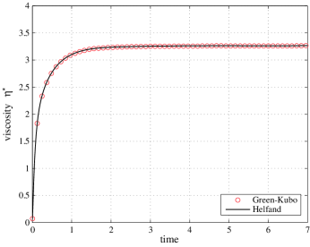
Figure 1: Viscosity at the phase point $T^{*}=0.722$ and $n^{*}=0.8442$ for $N=1372$. The plain line is the derivative of the mean-square displacement of the Helfand moment and the circles the integral of the microscopic flux autocorrelation function.

We depict in Fig. 1 the time derivative of the mean-square displacement of the Helfand moment (13) and the time integral of the autocorrelation function of the microscopic flux (11). In Fig. 1, the calculation is performed for $N=1372$ atoms near the triple point at the reduced temperature $T^{*}=0.722$ and density $n^{*}=0.8442$. As we see, the two method are in perfect agreement.

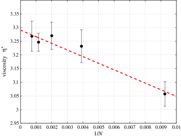
Figure 2: Viscosity at the phase point $T^{*}=0.722$ and $n^{*}=0.8442$ as a function of the inverse of the number $N$ of atoms. The circles are the results of the numerical simulations and the dashed line the linear extrapolation.

We estimated the shear viscosity by a linear fit on the mean-square displacement of the Helfand moment. The fit is done in the region between 5 and 10 time units to guarantee that the linear regime is reached. We depict in Fig. 2 the shear viscosity versus the inverse $N^{-1}$ of the system size. The linear extrapolation gives the following estimate of shear viscosity for an infinite system,

$$\eta^{*}=3.291\pm 0.057$$ (23)

This result is in agreement with the previous works as reported in Table 2. Indeed, the previous extrapolation found by Erpenbeck Erpenbeck (1988) $\eta^{*}=3.345\pm 0.068$, Palmer Palmer (1994) $\eta^{*}=3.25\pm 0.08$, and Meier et al. Meier et al. (2004) $\eta^{*}=3.258\pm 0.033$ are all in agreement with our result (23) within the statistical error.

Authors	year	method	$r_{\rm cut}^{*}$	$T^{*}$	$N$	$\eta^{*}$	$\Delta\eta^{*}$
Levesque et al. Levesque et al. (1973)	1973	GK (MD)	N. C.	0.722	864	4.03	0.3
Ashurst and Hoover Ashurst and Hoover (1973)	1973	SSW	N. C.	0.722	864	3.88	0.0026
Ashurst and Hoover Ashurst and Hoover (1975)	1975	SSW	N. C.	0.722	$\infty$	2.9	0.1
Hoover et al. Hoover et al. (1980)	1980	SSW	2.5	0.715	864	3.0	0.15
		OSW		0.722	108	3.18	0.1
Levesque a)	1980	GK (MD)	N. C.	0.728	108	2.97	N. C.
				0.715	256	2.92	N. C.
				0.722	864	3.85	N. C.
Pollock a)	1980	GK (MD)	N. C.	0.722	256	2.6	0.1
				0.722	500	3.2	0.2
Evans Evans (1981)	1981	LE	2.5	0.722	108-256 b)	3.17	0.03
Heyes Heyes (1983)	1983	DT	2.5	0.73	500	3.08	0.24
Schoen and Hoheisel Schoen and hoheisel (1985)	1985	GK (MD)	2.5	0.73	500	3.18	0.15
Erpenbeck Erpenbeck (1988)	1988	GK (MC)	2.5	0.722	108	2.912	0.071
					864	3.200	0.160
					$\infty$	3.345	0.068
Heyes Heyes (1988)	1988	GK (MD)	N. C.	0.72	108	3.2	0.16
					256	3.5	0.18
					500	3.4	0.17
Ferrario et al. Ferrario et al. (1991)	1991	GK (MD)	2.5	0.725	500	3.02	0.07
				0.7247	864	3.24	0.10
				0.725	864	3.11 - 3.27 c)	0.10
					2048	3.24	0.04
					4000	3.28	0.13
Palmer Palmer (1994)	1994	TCAF	2.5	0.722	$\infty$	3.25	0.08
Stassen and Steele Stassen and Steele (1995)	1995	GK (MD)	3.4	0.722	256	3.297	N. C.
Meier et al. Meier et al. (2004)	2004	GEF	2.5	0.722	108	2.984	0.089
			3.25		256	3.105	0.093
			4.0		500	3.188	0.096
			5.0		864	3.314	0.099
			2.5		1372	3.277	0.098
			5.5		2048	3.224	0.097
			5.5		4000	3.275	0.098
					$\infty$	3.258	0.033
This work	2007	HM (MD)	2.5	0.722	108	3.057	0.045
					256	3.232	0.060
					500	3.270	0.050
					864	3.247	0.033
					1372	3.268	0.055
					$\infty$	3.291	0.029

Table 2: Results found in the literature for the shear viscosity in the Lennard-Jones fluid near the triple point. The reduced density equals $n^{*}=0.8442$, except for the result reported by Heyes (1988) Heyes (1988) ($n^{*}=0.848$), and by Stassen and Steele Stassen and Steele (1995) ($n^{*}=0.8445$) . Abbreviations: DT, difference in trajectories method. GEF, generalized Einstein relation with integration of the flux. GK (MC), Green-Kubo results with Monte-Carlo method. GK (MD), Green-Kubo results with molecular dynamics. OSW, oscillatory shearing walls. SSW, steady shearing walls. TCAF, method based on the transverse-current autocorrelation functions. HM (MD) the present Helfand-moment method with molecular dynamics (MD). The infinite sign means that the value of the shear viscosity is obtained by extrapolation for $N\to\infty$. N. C. means that the value has not been communicated.
^a) Values unpublished but communicated by Hoover et al. Hoover et al. (1980).
^b) No size dependence.
^c) Values obtained for different thermostatting rates.

VI Conclusions

In this paper, we propose a new method for the computation of shear viscosity by molecular dynamics. The Helfand-moment method is an adaptation of the Helfand formula (3) for systems with periodic boundary conditions by adding two terms (12) to the original expression of the Helfand moment (4). The method consists in the calculation of the mean-square displacement of the Helfand moment (13). The variance of this quantity gives the shear viscosity by the generalized Einstein relation (3). We have discussed its validity in the light of the discussions found in the literature of the beginning of the nineties. Thanks to this new method, we have computed the shear viscosity in the Lennard-Jones fluid near the triple point. We showed that the Helfand-moment method gives the same results as the standard Green-Kubo method. Moreover, our extrapolated value of shear viscosity is in statistical agreement with those found in the literature. More than stating as an alternative method to the standard Green-Kubo in equilibrium molecular dynamics, the Helfand-moment method is useful and plays a central role in the escape-rate formalism and the hydrodynamic-mode method. Indeed, in these theories, the Helfand moment allows us to put in evidence fractal structures at the microscopic level, which are related to the transport processes Dorfman and Gaspard (1995); Gaspard and Dorfman (1995); Gaspard (1998); Dorfman (1999); Viscardy and Gaspard (2003b).

We remark that the method can be similarly extended to the bulk viscosity $\zeta$. As for the shear viscosity, two terms must be added to the original expression of the Helfand moment associated with the bulk viscosity. Formally, this last coefficient is expressed as follows:

$$\zeta+\frac{4}{3}\eta=\lim_{N,V,t\to\infty}\frac{1}{2k_{\rm B}TVt}\left\langle\left[G^{(\zeta)}(t)-\langle G^{(\zeta)}(t)\rangle\right]^{2}\right\rangle,$$ (24)

where its Helfand moment is defined as:

$$G^{(\zeta)}(t) = \sum_{a}p_{ax}(t)\;x_{a}(t)$$ (25)

$$- \sum_{a}\sum_{s}p_{ax}^{(s)}\;\Delta x_{a}^{(s)}\;\theta(t-t_{s})$$

$$- \frac{1}{2}\sum_{a\neq b}\int_{0}^{t}d\tau\;F_{x}({\bf r}_{ab})\;L_{b|ax}\,,$$

and with $G^{(\zeta)}(0)=0$. In the companion paper, we will present a similar method for the calculation of thermal conductivity Viscardy et al. .

Appendix A Derivation of the Helfand moment for the shear viscosity in periodic systems

By taking the time derivative of the Helfand moment (10), we have:

$$\frac{dG^{(\eta)}(t)}{dt} = \sum_{a}\frac{p_{ax}(t)p_{ay}(t)}{m}$$ (26)

$$+ \sum_{a}\sum_{s}p_{ax}(t)\Delta y_{a}^{(s)}\delta(t-t_{s})$$

$$+ \sum_{a\neq b}F_{x}(\mathbf{r}_{ab})y_{a}(t)+\frac{dI(t)}{dt}$$

where we have used the modified Newton equations (9). The term implying the interparticle force $\mathbf{F}({\bf r}_{ab})$ may be modified into

$$\sum_{a\neq b}F_{x}(\mathbf{r}_{ab})y_{a}(t)=\frac{1}{2}\sum_{a\neq b}F_{x}({\bf r}_{ab})y_{a}+\frac{1}{2}\sum_{a\neq b}F_{x}({\bf r}_{ba})y_{b}\,.$$ (27)

Since the force $\mathbf{F}$ is central, we obtain $F_{x}({\bf r}_{ab})=-F_{x}({\bf r}_{ba})$, which implies that

$$\sum_{a\neq b}F_{x}(\mathbf{r}_{ab})y_{a}(t)=\frac{1}{2}\sum_{a\neq b}F_{x}({\bf r}_{ab})\,(y_{a}-y_{b})\,.$$ (28)

which still differs from the corresponding term appearing in the microscopic flux (11) defined with the minimum-image convention because $y_{a}-y_{b}=y_{ab}+L_{b|ay}$ according to Eqs. (7) and (8). Consequently, Eq. (26) becomes

$$\frac{dG^{(\eta)}(t)}{dt} = J^{(\eta)}(t)+\frac{1}{2}\sum_{a,b\neq a}F_{x}({\bf r}_{ab})L_{b|ay}$$

$$+ \sum_{a}\sum_{s}p_{ax}(t)\Delta y_{a}^{(s)}\delta(t-t_{s})+\frac{dI(t)}{dt}\,.$$

Comparing with Eq. (5), we should have

$$\frac{dI(t)}{dt} = -\sum_{a}\sum_{s}p_{ax}(t)\Delta y_{a}^{(s)}\delta(t-t_{s})$$ (30)

$$- \frac{1}{2}\sum_{a,b\neq a}F_{x}({\bf r}_{ab})L_{b|ay}$$

whereupon $I(t)$ can be expressed as

$$I(t) = -\sum_{a}\sum_{s}p_{ax}^{(s)}\Delta y_{a}^{(s)}\theta(t-t_{s})$$ (31)

$$- \frac{1}{2}\sum_{a,b\neq a}\int_{0}^{t}d\tau\;F_{x}({\bf r}_{ab})\;L_{b|ay}\;.$$

References

- (1)
- Maxwell (1860) J. Maxwell, Phil. Mag. 19, 19 (1860).
- (3) S. Viscardy, E-print: cond-mat/0601210.
- Green (1951) M. S. Green, J. Chem. Phys. 19, 1036 (1951).
- Green (1960) M. S. Green, Phys. Rev. 119, 829 (1960).
- Kubo (1957) R. Kubo, J. Phys. Soc. Jpn. 12, 570 (1957).
- Mori (1958) H. Mori, Phys. Rev. 112, 1829 (1958).
- Helfand (1960) E. Helfand, Phys. Rev. 119, 1 (1960).
- Alder et al. (1970) B. J. Alder, D. M. Gass, and T. E. Wainwright, J. Chem. Phys. 53, 3813 (1970).
- Levesque et al. (1973) D. Levesque, L. Verlet, and J. Kürkijarvi, Phys. Rev. A 7, 1690 (1973).
- Schoen and hoheisel (1985) M. Schoen and C. hoheisel, Mol. Phys. 56, 653 (1985).
- Erpenbeck (1988) J. J. Erpenbeck, Phys. Rev. A 38, 6255 (1988).
- Lees and Edwards (1972) A. W. Lees and S. F. Edwards, J. Phys. C 5, 1921 (1972).
- Ashurst and Hoover (1973) W. T. Ashurst and W. G. Hoover, Phys. Rev. Lett. 31, 206 (1973).
- Hoover et al. (1980) W. G. Hoover, D. J. Evans, R. B. Hickman, A. J. C. Ladd, W. T. Ashurst, and B. Moran, Phys. Rev. A 22, 1690 (1980).
- Evans (1981) D. J. Evans, Phys. Rev. A 23, 1988 (1981).
- Trozzi and Ciccotti (1984) C. Trozzi and G. Ciccotti, Phys. Rev. A 29, 916 (1984).
- Allen (1993) M. P. Allen, in Computer Simulation in Chemical Physics, edited by M. P. Allen and D. J. Tildesley (Kluwer, Amsterdam, 1993), pp. 49–92.
- Haile (1997) J. M. Haile, Molecular Dynamics Simulation (John Wiley & Sons, New York, 1997).
- Meier et al. (2004) K. Meier, A. Laesecke, and S. Kabelac, J. Chem. Phys. 121, 3671 (2004).
- Hess and Evans (2001) S. Hess and D. J. Evans, Phys. Rev. E 64, 011207 (2001).
- McQuarrie (2000) D. McQuarrie, Statistical Mechanics (University Science Books, Sausalito, 2000).
- Chialvo and Debenedetti (1991) A. A. Chialvo and P. G. Debenedetti, Phys. Rev. A 43, 4289 (1991).
- Chialvo et al. (1993) A. A. Chialvo, P. T. Cummings, and D. J. Evans, Phys. Rev. E 47, 1702 (1993).
- Allen et al. (1994) M. P. Allen, D. Brown, and A. J. Masters, Phys. Rev. E 49, 2488 (1994).
- Allen (1994) M. Allen, Phys. Rev. E 50, 3277 (1994).
- Erpenbeck (1995) J. J. Erpenbeck, Phys. Rev. E 51, 4296 (1995).
- Viscardy and Gaspard (2003a) S. Viscardy and P. Gaspard, Phys. Rev. E 68, 041204 (2003a).
- Dorfman and Gaspard (1995) J. R. Dorfman and P. Gaspard, Phys. Rev. E 51, 28 (1995).
- Gaspard and Dorfman (1995) P. Gaspard and J. R. Dorfman, Phys. Rev. E 52, 3525 (1995).
- Gaspard (1998) P. Gaspard, Chaos, Scattering and Statistical Mechanics (Cambridge University Press, Cambridge, 1998).
- Dorfman (1999) J. R. Dorfman, An Introduction to Chaos in Nonequilibrium Statistical Mechanics (Cambridge University Press, Cambridge, 1999).
- Viscardy and Gaspard (2003b) S. Viscardy and P. Gaspard, Phys. Rev. E 68, 041205 (2003b).
- Gaspard (1996) P. Gaspard, Phys. Rev. E 53, 4379 (1996).
- Einstein (1905) A. Einstein, Ann. d. Phys. 17, 549 (1905), translated and reprinted in Investigations on the theory of the brownian movement (Dover, New York, 1956).
- (36) Eq. (3.13) in Helfand’s paper Helfand (1960) and Eq. (21-304) in McQuarrie’s book McQuarrie (2000).
- Hess et al. (2003) S. Hess, M. Kröger, and D. Evans, Phys. Rev. E 67, 042201 (2003).
- Meier et al. (2005) K. Meier, A. Laesecke, and S. Kabelac, J. Chem. Phys. 122, 014513 (2005).
- Swope et al. (1982) W. C. Swope, H. C. Andersen, P. H. Berens, and K. R. Wilson, J. Chem. Phys. 76, 637 (1982).
- Palmer (1994) B. J. Palmer, Phys. Rev. E 49, 359 (1994).
- Ashurst and Hoover (1975) W. T. Ashurst and W. G. Hoover, Phys. Rev. A 11, 658 (1975).
- Heyes (1983) D. M. Heyes, J. Chem. Soc. Faraday Trans. 79, 1741 (1983).
- Heyes (1988) D. M. Heyes, Phys. Rev. B 37, 5677 (1988).
- Ferrario et al. (1991) M. Ferrario, G. Ciccotti, B. L. Holian, and J. P. Ryckaert, Phys. Rev. A 44, 6936 (1991).
- Stassen and Steele (1995) H. Stassen and W. A. Steele, J. Chem. Phys. 102, 932 (1995).
- (46) S. Viscardy, J. Servantie, and P. Gaspard, companion paper to appear (2007).