Orientational Ordering and Dynamics of Rodlike Polyelectrolytes

Abstract

The interplay between electrostatic interactions and orientational correlations is studied for a model system of charged rods positioned on a chain, using Monte Carlo simulation techniques. It is shown that the coupling brings about the notion of electrostatic frustration, which in turn results in: (i) a rich variety of novel orientational orderings such as chiral phases, and (ii) an inherently slow dynamics characterized by stretched-exponential behavior in the relaxation functions of the system.

I Introduction

Solutions of highly charged polymers are known to develop novel structural properties due to the interplay between electrostatic interactions and entropic effects gelbart . For example, it has been shown that for most charged biopolymers such as DNA, filamentous (F-)actin, and various viruses DNA-collapse , electrostatic correlations in the vicinity of the macroions caused by multivalent counterions—ions of opposite charge—can lead to like-charged attraction levin . This attraction most often destabilizes the polyelectrolyte solution and leads to the formation of collapsed bundles.

In a recent experiment with F-actin, Wong et al. observed that when the density of multivalent counterions is not yet sufficient to trigger complete collapse, the uniform solution can become unstable and phase separate into coexisting low- and high-density phases gerard . This experiment is perhaps a most direct manifestation of the peculiar behavior of polyelectrolytes in high density solutions: the dense phase is characterized by multi-axial liquid crystalline behavior itamar , as well as exceedingly slow dynamics that leads to the formation of an actin gel gerard . A similar self-assembly pattern has been observed in the structure of the nuclear lamina—a charged filamentous integral membrane protein network that provides a cytoskeletal support for the nuclear membrane alb .

Another interesting example is the observation of slow modes in the dynamics of various high-density polyelectrolyte solutions in the absence of salt, where it is suggested that correlations cause the formation of starlike complexes with considerably slow dynamics slow ; muthu . These examples raise the issue that strong many-body Coulombic correlations for extended (non-pointlike) charged objects could lead to novel features that are poorly understood.

Based on such experimental evidence, one can broadly identify two characteristic features in this class of problems: the novel orientational ordering, and the slow dynamics. As a first step towards understanding such properties, one should note the frustration that is inherent structurally in the collection of like-charged rodlike objects: As they come together, they reorient themselves to minimize the total energy of the system. Here, the long range nature of the interaction presents them with a multitude of configurations that are good minimum energy candidates and yet are far apart in the configuration space. This picture is partly supported by the fact that there are so many of them. This picture is supported by the fact that in the presence of (a considerable amount of) salt the above effects are washed out, as screening can eliminate the frustration by reducing the effective range of the mutual repulsion.

Here, we set out to study the collective behavior of polyelectrolytes at close separations using Monte Carlo (MC) simulation, with the primary goal of understanding the complexity that electrostatic frustration can bring about. We consider a most simple model system of similarly charged rigid rods of equal length $L$ with their centers forming a regular lattice of spacing $a$ on a chain, as shown in Fig. 1. We find a variety of collective behaviors, and map out the phase diagram for the system as a function of temperature and lattice spacing (inverse density of the rods), as shown in Fig. 2. In the low-density regime, the rods are found to order in a staggered way upon decreasing the temperature, such that they are perpendicular both to their neighbors and to the axis that connects their centers, through a two-stage crossover transition.

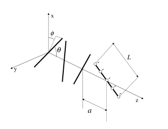
Figure 1: The schematic configuration of charged rods. The centers of the rods of equal length $L$ are fixed on a chain of spacing $a$. Each rod has two rotational degrees of freedom, and a uniform distribution of point charges.

For intermediate densities, we find that a low-temperature ordered phase appears through a first-order phase transition, in which neighboring rods have a twist angle in addition to the ninety degrees of the low-density phase. In the high-density regime, a hierarchy of different phases is observed depending on the lattice spacing, where there is a multitude of twist angles, a periodic structure with a basis, and out-of-plane arrangements of the rods. We also study the equilibrium relaxation properties of the system and find that the appropriate order parameter in the system has an anomalous relaxation characterized by a stretched-exponential behavior, which is a feature also seen in systems with frustration.

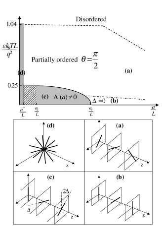
Figure 2: Phase diagram of the system in the $a-T$ plane. Dashed line: The crossover transition line from a disordered regime to partially ordered one [region (a)]. Dash-dotted line: The crossover transition line from a partially ordered regime to the staggered ground-state of the low-density regime [region (b)]. Solid line: First order transition line from a partially ordered regime to the chiral ordered phase of the intermediate-density case [region (c)]. Hashed region: The domain in which a multitude of transitions occur to phases with various kinds of orderings. Region (d): The “sea urchin” phase. Schematic configuration of rods corresponding to the different parts of the phase diagram is indicated in the lower panel. The values of the various transition points indicated in the phase diagram are $a_{c}=0.40\,L$, $a_{1}=0.10\,L$, and $a^{*}\simeq 0.02\,L$.

The rest of the paper is organized as follows. In Sec. II, we introduce the model and outline the simulation technique used. Section III is devoted to the description of various parts of the phase diagram, which is followed by discussions on the relaxation dynamics of the system in Sec. IV. Some discussions and concluding remarks are presented in Sec. V. Finally, a variant of the model that corresponds to polyelectrolyte combs is discussed in the Appendix.

II The Model

We use the Metropolis algorithm to simulate a system of $N_{r}$ rods with their centers fixed on a chain, and only their rotational degrees of freedom $(\theta,\phi)$ left to explore theta . We assume that $N_{q}$ (odd) point-charges of the same sign are distributed symmetrically on each rod (Fig. 1). The screened Coulomb interaction energy of the system of rods can be written as:

$$U=\frac{q^{2}}{\varepsilon}\sum_{m>n}^{N_{r}}\sum_{i,j=1}^{N_{q}}\frac{e^{-\kappa|{{\bf r}_{mi}-{\bf r}_{nj}}|}}{|{{\bf r}_{mi}-{\bf r}_{nj}}|},$$ (1)

where $\varepsilon$ is the dielectric constant of the medium, $q=Q/N_{q}$ where $Q$ is the overall charge of the rod, ${\bf r}_{mi}({\bf r}_{nj})$ is the position of charge $i(j)$ on rod $m(n)$, and $\kappa^{-1}$ is the Debye screening length. Note that the energy expression is invariant under the local transformation $\theta\to\pi-\theta$ and $\phi\to\phi+\pi$ for each rod. We use free boundary conditions to avoid complexities arising from the Ewald-summation of extended charge distributions Ewald .

For each value of the lattice constant $a$, we start the system from a random configuration of the rods at a high temperature (where the system is in the disordered phase) and gradually cool down toward lower temperatures. At a given temperature, we start the calculation of various thermal averages after equilibration and take the last configuration at each temperature as the initial configuration for a slightly lower temperature. We have run a wide variety of simulations for different values of $N_{r}$, $N_{q}$, and $a$, and found that all the qualitative results are robust.

III The Phase Diagram

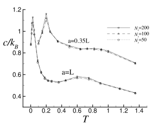
Figure 3: The specific heat as a function of temperature $T$ [in units of $q^{2}/(\varepsilon k_{\rm B}L)$] for (a) $a=L$ and (b) $a=0.35\,L$, with three different sizes $N_{r}=50,\,100,\,200$ and $N_{q}=3$.

To capture the essence of the electrostatic frustration, we first consider the salt-free case that corresponds to $\kappa=0$, and comment on the effect of screening later. In Fig. 2, we show the phase diagram of the system in the plane of temperature and lattice constant for $N_{r}=100$ and $N_{q}=3$.

In the low-density regime, where $a$ is greater than a critical value $a_{c}=0.40\,L$, the rods appear to order on decreasing the temperature through a two-stage crossover transition. The first crossover (denoted by the dashed line in Fig. 2) takes the system to a partially ordered phase in which the angular degree of freedom, $\theta$, freezes to $\frac{\pi}{2}$, and the rods fluctuate freely only within the resulting parallel plates [region (a) in Fig. 2]. The ordering in the $\phi$ degree of freedom occurs through another crossover at a lower temperature (denoted by the dash-dotted line in Fig. 2). The crossover transition temperatures are determined from the specific heat of the system as a function of temperature, which develops two rounded peaks. In Fig. 3a, the specific heat of the system is plotted as a function of the temperature $T$, which is made dimensionless by the combination $q^{2}/(\varepsilon k_{\rm B}L)$, at $a=L$ for three different sizes $N_{r}=50,\,100,\,200$ and $N_{q}=3$. Each data point is the average over five independent runs starting from different initial random configurations. For each temperature, $1.5\times 10^{6}$ MCS are used with the first $7.5\times 10^{5}$ MCS being for equilibration. As can be seen from Fig. 3a, the height of the peaks in the specific heat do not change appreciably for various values of the system size $N_{r}=50,\,100,\,200$.

The ground-state configuration corresponding to this regime is given as [see Fig. 2b]:

$$\theta_{m}=\frac{\pi}{2}~{}~{}{\rm and}~{}~{}\phi_{m}=m\times\frac{\pi}{2},$$ (2)

where $m$ indicates the position of the centers of rods on the $z$ axis $(z_{m}=ma)$. This is in agreement with the two-body minimum energy configuration of the rods adrian . A multipole expansion of the electrostatic energy expression in Eq. (1), which is presumably a good approximation in the limit of $a\gg L$, reveals that the system of rods effectively behaves as a collection of quadrupoles in an external staggered electric field; hence the perpendicular ordering described by Eq. (2). This picture also agrees well with the lack of genuine phase transitions in this regime, as it is expected from quadrupoles in a symmetry breaking external field.

In the intermediate-density regime, corresponding to $a^{*}<a<a_{c}$ where $a^{*}\simeq 0.025\,L$, lowering the temperature for each value of the lattice constant causes a crossover transition from disordered to partially ordered regime, which is followed by a phase transition (solid line in the phase diagram in Fig. 2) to low-temperature phases having chiral order. A plot for the specific heat in this regime, corresponding to $a=0.35\,L$, is shown in Fig. 3b for system sizes $N_{r}=50,\,100,\,200$ and $N_{q}=3$. The data points are the averages of five independent runs starting from different initial random configurations. For each temperature $2\times 10^{6}$ MCS are used, with $10^{6}$ MCS being for equilibration. It can again be seen that the specific heat is not sensitive to the size of the system.

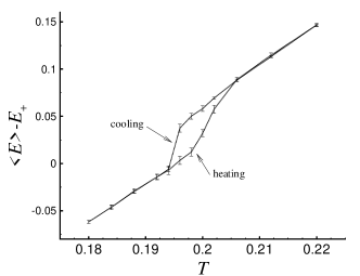
Figure 4: The thermal average of energy per site [in units of $q^{2}/(\varepsilon L)$] as a function of the temperature [in units of $q^{2}/(\varepsilon k_{\rm B}L)$] upon successive cooling and heating of the system, for $a=0.35\,L$, $N_{r}=100$, $N_{q}=3$. The self-energy of the staggered ground-state configuration $E_{+}$ is subtracted off from the energy. The hysteresis loop can be observed, which indicates a first order transition from the partially ordered regime to the chiral phase.

To understand the nature of the phase transition, we examined the energy of the system upon successive cooling and heating. In Fig. 4, the thermal average of energy per site as a function of the temperature [that is made dimensionless using $q^{2}/(\varepsilon k_{\rm B}L)$] is plotted for $a=0.35\,L$ corresponding to successive cooling and heating of the system. In this curve, $7.5\times 10^{5}$ MCS are used for equilibration and $7.5\times 10^{5}$ MCS for ensemble averages, and it corresponds to $N_{r}=100$, $N_{q}=3$. As can be seen from Fig. 4, the average energy of the system shows hysteresis around the transition temperature, which is a signature of a first order phase transition. One can also define an order parameter that could distinguish between the two phases and thus monitor the phase transition as a function of temperature. A suitable choice for the order parameter could be

$$M=\frac{1}{N_{r}-1}\sum_{n=1}^{N_{r}-1}\langle\sin\Delta_{n}\rangle,$$ (3)

where $\Delta_{n}(t)=\phi_{n+1}(t)-\phi_{n}(t)-\frac{\pi}{2}$. Figure 5 shows a plot of this order parameter versus temperature [in units of $q^{2}/(\varepsilon k_{\rm B}L)$] for a system of $N_{r}=200$ and $N_{q}=3$ at $a=0.35\,L$. In this plot, $10^{6}$ MCS are used for equilibration of the system and $10^{6}$ MCS for thermal averages. It can be seen that the order parameter develops a discontinuous jump across the transition temperature. This is another indication that the transition across the solid line in the phase diagram of Fig. 2 is first order. These observations, however, should be complemented with more systematic investigations using energy histogram methods LK ; future .

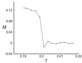
Figure 5: The order parameter $M$ [defined in Eq. (3)] versus temperature [in units of $q^{2}/(\varepsilon k_{\rm B}L)$] for a system of $N_{r}=200$, $N_{q}=3$ at $a=0.35\,L$.

Below this transition, the system of rods appears to develop a rich variety of orderings. For $a_{1}<a<a_{c}$ where $a_{1}=0.1\,L$ [region (c) in the phase diagram in Fig. 2], the array of rods orders in a chiral phase with the corresponding ground-state configuration given as:

$$\theta_{m}=\frac{\pi}{2}~{}~{}{\rm and}~{}~{}\phi_{m}=m\times\left(\frac{\pi}{2}+\Delta_{g}(a)\right).$$ (4)

Since the twist angle $\Delta$ is small in the vicinity of the transition line, we can simplify our description by assuming that $\Delta$ itself serves as the corresponding order parameter for the phase transition from (a) and (b) to (c). While its value is observed to undergo a finite jump just below the transition line, the ground-state value $\Delta_{g}(a)$ is found to vanish continuously at $a_{c}$, implying that the termination point of the transition line at zero temperature corresponding to $a=a_{c}$ is a critical point.

For a more direct study of the transition in the ground-state configuration at $a_{c}$, we calculate the exact energy per site for the system using the energy expression given in Eq. (1) as a function of $\Delta$ for the configuration given in Eq. (4). This means that we freeze the charged rods into the configurations defined by Eq. (4) and calculated in a point by point double summation the electrostatic energy of the configuration for each value of $\Delta$. This energy function, which is plotted in Fig. 6 for different values of $a$, admits a Landau form and the corresponding minimum energy solution $\Delta_{g}(a)$ vanishes at $a_{c}$ as $\Delta_{g}=|a_{c}-a|^{\beta}$ with $\beta=0.500$ (see inset of Fig. 6). We have checked that the value of $\beta$ does not depend on $N_{q}$ (even up to $N_{q}=1001$), confirming the expectation from Landau theory that $\beta=1/2$.

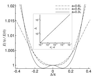
Figure 6: A plot of the ground-state energy per site as a function of $\Delta$ for $a=0.3\,L$, $a=a_{c}=0.4\,L$, and $a=0.6\,L$, with $N_{r}=40$ and $N_{q}=3$. The value of $\Delta$ which minimizes the energy of the system vanishes continuously at $a=a_{c}$. Inset: The log-log plot of $\Delta_{g}$ versus $(a_{c}-a)$ gives a slope of $\beta=0.500$.

In the intermediate-density regime when the rods are brought closer to each other, different configurations that are close in energy appear. This changes the behavior of the system at $a_{1}$ where the curve of energy versus $\Delta$ starts to have four degenerate minima. For $a^{*}<a<a_{1}$ with $a^{*}\simeq 0.025\,L$ (hashed region in Fig. 2), while the rods still respect the planar ordering, a multitude of transitions occur taking the system through a variety of minimum energy configurations. For example, upon increasing the density, a phase appears in which successive cross-like structures formed by two neighboring rods are rotated relative to each other around the $z$-axis by an angle $\Delta^{\prime}$, which corresponds to a chiral ordering with a basis. Finally, in the high-density region where $a<a^{*}$, the rods are no longer confined in the planes. While in this regime one also finds various kinds of orderings, eventually the rods tend to approach a spherical configuration that resembles a “sea urchin” [see Fig. 2(d)], as $a$ approaches its smallest possible value $a_{0}$ that is set by the thickness of the rods. Note that only a very small choice of the cutoff length, such as our choice of $a_{0}=10^{-6}\,L$, can allow for these complicated high-density phases to exist. Moreover, unlike the lower density cases, this part of the phase diagram depends very sensitively on the choice of charge distribution on the rods, namely the value of $N_{q}$ as well as whether the charges are smeared or discrete.

IV Relaxation Dynamics

The low-temperature chiral ordering (in either of its various forms) is not easily achieved in its complete form when the system is cooled down from the disordered phase to temperatures below the transition line. This means that the equilibrium dynamics of the system involves a rather slow process, which we try to identify and study here.

For $a_{1}<a<a_{c}$, the array of rods is decomposed into several domains of the chiral structure with both positive and negative values of $\Delta$, corresponding to the degenerate minima of energy shown in Fig. 6. The neighboring left-handed and right-handed domains are regions that typically contain just a few rods, and are linked via what can be thought of as kinks. By definition, the kinks annihilate when they meet each other or when they reach the boundaries of the system. We observe that the density of the kinks is more or less fixed to about one kink for every 40 rods or so, irrespective of the size of the system.

These kinks are observed to have very slow dynamics, presumably due to the electrostatic frustration, so that a considerably long MC time is needed before all the kinks are annihilated and one of the domains spans the entire system. The MC time needed for the annihilation of the kinks increases with increasing the system size. We also note that when the energy has four minima (for $a$ just below $a_{1}$) and two kinds of chiral structures are possible, different kinds of kinks are observed depending on the type of the two neighboring domains that are linked.

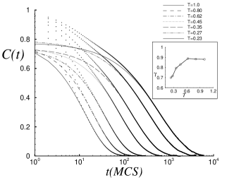
Figure 7: Equilibrium relaxation function of the system for $a=0.25\,L$ and various temperatures, reported in units of $q^{2}/(\varepsilon k_{\rm B}L)$. The nonlinear fits to the long-time behavior of the curves are of the stretched-exponential form. Inset: A plot of $\gamma$ as a function of temperature.

To put the study of the slow dynamics in a more quantitative framework, we probe the equilibrium relaxation properties of the system by measuring the auto-correlation function for $\Delta_{n}(t)$, which is defined as:

$$C(t)=\frac{\sum_{n=1}^{N_{r}-1}{\int dt^{\prime}\Delta_{n}(t+t^{\prime})\Delta_{n}(t^{\prime})}}{\sum_{n=1}^{N_{r}-1}{\int dt^{\prime}\Delta_{n}(t^{\prime})\Delta_{n}(t^{\prime})}}.$$ (5)

To obtain $C(t)$ at each temperature $T$, we start the system from a random configuration at high temperatures and quench it to $T$. After running the system for a waiting time, $t_{w}$, we use the system configuration $\phi_{n}(t)$ in all time steps from $t_{w}$ to $t_{w}+t_{av}$ to calculate $C(t)$ using Eq. (5). For long enough waiting times ($t_{w}\simeq 2\times 10^{6}$ MC steps for $N_{r}=100$)), the relaxation function $C(t)$ is independent of $t_{w}$ as well as the system initial conditions, indicating that there is no difference between averaging over time [Eq. (5)] and averaging over different initial conditions of the system. Note that the waiting time is typically the time needed for the kinks to annihilate.

In Fig. 7, we show the system relaxation function with logarithmic time scale for different values of temperature in the case of $a=0.25\,L$ with $N_{r}=100$ and $N_{q}=3$. Using nonlinear fits with three free parameters, we find that the long-time part of the relaxation function is well represented by the stretched-exponential form, $C_{0}\,\exp[-(t/\tau)^{\gamma}]$. The exponent $\gamma$ saturates to a constant of the order of $0.9$ in the high temperature regime, while it drops at lower temperatures where the relaxation is exceedingly slower. The stretched-exponential form for the relaxation is a feature that is often encountered in the dynamics of frustrated systems frustrated .

V Discussion and Conclusion

In a most simple realization of the system, we have shown that charged linear objects in close separation can develop novel collective orientational correlations as well as an unusually slow dynamics, due to the frustration in the orientational degrees of freedom. While in our simple model system we assume that the rods are positioned in a lattice, we expect that removing this constraint will cause the orientational correlations to manifest themselves as liquid crystalline structures such as those observed in Ref. gerard . Geometrical frustration induced by the dimensionality of the arrangement could also affect the orientational ordering, and it remains to be seen what kind of arrangement is favored by the liquid system itself, i.e., what is the coupling between the positional- and the orientational correlations in this frustrated system.

Let us examine the effect of screening by added-salt in the above results. For a low concentration of added salt, the screening is weak and we expect that the results reported here will hold true so long as the screening length is the largest length in the system. As the salt concentration is increased, however, the Debye length begins to compete with the other length scales and this could change the phase behavior of the system.

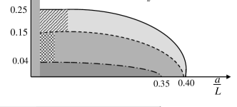
Figure 8: First order transition line of the phase diagram for different values of the screening parameter.

We have performed simulations with the screened Coulomb interaction of Eq. (1) using different values for the Debye screening length. We find that the general structure of the phase diagram of Fig. 2 persists, while the size of the chiral domain in the phase diagram shrinks as $\kappa$ is increased. In Fig. 8, the first order phase transition line is shown for three values of the Debye length for $N_{r}=100$ and $N_{q}=3$. It can be seen that even for $\kappa^{-1}=L$ the value of $a_{c}$ barely changes as compared to its $\kappa=0$ value of $0.4\,L$. Our results suggest that $\kappa^{-1}\sim a_{c}$ sets the threshold where screening can wipe out the chiral ordering altogether.

We have neglected the effect of counterions in the above study. This can be justified by noting that the polyelectrolytes are very short rods and unless we choose extremely high values for $q$, it is unlikely that they condense on the rods. This means that they will move relatively freely in the vicinity of the linear polyelectrolyte array, and merely participate in the Debye screening of the interaction. This effect can be taken into account by considering a local effective value for the Debye length that incorporates the density of the counterions as well as that of salt. Moreover, the presence of the counterions in an effective “cell” around the array provides the necessary neutralization of the system. In our treatment, however, we did not need to care about the neutralization criterion because the centers of the charged rods are fixed in space and in effect it is only multipoles (not monopoles) that are interacting.

Finally, we note that the results obtained here are related to the studies of the equilibrium configuration of ions in a confined plasma, where even similar chiral phases are observed as the confinement potential becomes anisotropic plasma .

Appendix A End-grafted Charged Rods

In this Appendix, we consider the case where the charged rods are actually grafted at their ends instead of the mid-points. This will make a model for a polyelectrolyte comb, i.e. a backbone with a linear array of charged side chains, which has in fact been synthesized and studied comb ; waigh .

We have performed simulations on such a system and have found the same general behavior as the previous case. The corresponding phase diagram for the case of $N_{q}=7$ is shown in Fig. 9, where the transition points are found to be $a_{c}=1.40\,L$, and $a_{1}=0.3\,L$. Note that the region (b) in Fig. 9 corresponds to rods that are anti-parallel to their neighbors, which is a direct consequence of the non-vanishing dipole moment of rods that are grafted at one end as opposed to those that are grafted from the mid-point. Consequently, region (b) in this case corresponds to dipoles in a staggered field. Similarly, in the chiral phase the neighboring rods are out of phase by $\pi$ (instead of $\pi/2$) plus a residual twist angle. We also note that the transitions are occurring at larger values of the reduced temperature and lattice spacing, because of the stronger dipolar interactions.

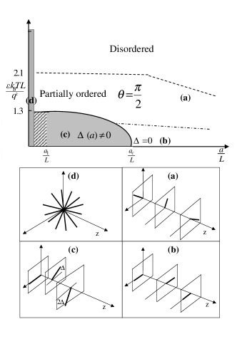
Figure 9: Phase diagram of the polyelectrolyte comb model in the $a-T$ plane. Dashed line: The crossover transition line from a disordered regime to partially ordered one [region (a)]. Dash-dotted line: The crossover transition line from a partially ordered regime to the staggered ground-state of the low-density regime [region (b)]. Solid line: First order transition line from a partially ordered regime to the chiral ordered phase of the intermediate-density case [region (c)]. Hashed region: The domain in which a multitude of transitions occur to phases with various kinds of orderings. Region (d): The “sea urchin” phase. Schematic configuration of rods corresponding to the different parts of the phase diagram is indicated in the lower panel. The values of the various transition points indicated in the phase diagram are $a_{c}=1.40\,L$ and $a_{1}=0.3\,L$.

References

- (1) W.M. Gelbart, R.F. Bruinsma, P.A. Pincus, and V.A. Parsegian, Physics Today 53, 38 (2000).
- (2) V.A. Bloomfield, Biopolymers 31, 1471 (1991); Curr. Opin. Struc. Biol. 6, 334 (1996); J.X. Tang and P.A. Janmey, J. Biol. Chem. 271, 8556 (1996); R. Podgornik, D. Rau, and V.A. Parsegian, Biophys. J. 66, 962 (1994).
- (3) For a recent review see: Y. Levin, Rep. Prog. Phys. 65, 1577 (2002).
- (4) G.C.L. Wong, A. Lin, J.X. Tang, Y. Li, P.A. Janmey, and C.R. Safinya, Phys. Rev. Lett. 91, 018103 (2003).
- (5) I. Borukhov and R.F. Bruinsma, Phys. Rev. Lett. 87, 158101 (2001).
- (6) B. Alberts, J. Lewis, M. Raff, K. Roberts, and J.D. Watson, Molecular Biology of the Cell, (Garland, New York, 1994).
- (7) For a review, see e.g.: D.F. Hodgson and E.J. Amis, in Polyelectrolytes: Science and Technology edited by M. Hara (Marcel Dekker, New York, 1992).
- (8) M. Muthukumar, J. Chem. Phys. 107, 2619 (1997).
- (9) In sampling the unit sphere described by uniformly, one should be careful to include the factor in the measure. In most interesting domains in the phase diagram of Fig. 2, however, the tendency to keep the rods in-plane makes this factor dispensible, as our explicit checks have shown.
- (10) M. Deserno and C. Holm, J. Chem. Phys. 109, 7678 (1998).
- (11) V.A. Parsegian, J. Chem. Phys. 56, 4393 (1972).
- (12) J. Lee and J.M. Kosterlitz, Phys. Rev. Lett. 65, 137 (1990).
- (13) H. Fazli, B. Farnudi, R. Golestanian, and M.R. Kolahchi, work in progress.
- (14) See e.g.: B. Kim and S.J. Lee, Phys. Rev. Lett. 78, 3709 (1997). Note that works as an inherent frustration parameter , and characterizes region (c) of the phase diagram (Fig. 2) as the frustrated phase.
- (15) C.P. Whitby, P.J. Scales, F. Grieser, T.W. Healy, G. Kirby, J.A. Lewis, and C.F. Zukoski, Journal of Colloid and Interface Science 262, 274 (2003).
- (16) T.A. Waigh, private communication.
- (17) See: J.P. Schiffer, in Strongly Coupled Coulomb Systems edited by G.J. Kalman et al. (Plenum Press, New York, 1998); and references therein.