Phase diagram and spin Hamiltonian of weakly-coupled
anisotropic ${\bf S=\frac{1}{2}}$ chains in ${\bf CuCl_{2}\cdot 2((CD_{3})_{2}SO)}$

Abstract

Field-dependent specific heat and neutron scattering measurements were used to explore the antiferromagnetic $S$=$\frac{1}{2}$ chain compound ${\rm CuCl_{2}\cdot 2((CD_{3})_{2}SO)}$. At zero field the system acquires magnetic long-range order below $T_{N}=0.93\;\mathrm{K}$ with an ordered moment of $0.44\mu_{B}$. An external field along the b-axis strengthens the zero-field magnetic order, while fields along the a- and c-axes lead to a collapse of the exchange stabilized order at $\mu_{0}H_{c}=6\;\mathrm{T}$ and $\mu_{0}H_{c}=3.5\;\mathrm{T}$, respectively (for $T=0.65\;\mathrm{K}$) and the formation of an energy gap in the excitation spectrum. We relate the field-induced gap to the presence of a staggered g-tensor and Dzyaloshinskii-Moriya interactions, which lead to effective staggered fields for magnetic fields applied along the a- and c-axes. Competition between anisotropy, inter-chain interactions and staggered fields leads to a succession of three phases as a function of field applied along the c-axis. For fields greater than $\mu_{0}H_{c}$, we find a magnetic structure that reflects the symmetry of the staggered fields. The critical exponent, $\beta$, of the temperature driven phase transitions are indistinguishable from those of the three-dimensional Heisenberg magnet, while measurements for transitions driven by quantum fluctuations produce larger values of $\beta$.

I Introduction

Weakly-coupled antiferromagnetic (AF) $S=\frac{1}{2}$ chains can be close to one or several quantum critical points and serve as interesting model systems in which to explore strongly-correlated quantum order. An isolated AF $S=\frac{1}{2}$ Heisenberg chain, described by

$${\mathcal{H}}=J\sum_{n}{\bf S}_{n}\cdot{\bf S}_{n+1}\,,$$ (1)

is quantum critical at zero temperature. Due to the absence of a length scale at a critical point, the spin correlations decay as a power law, and the fundamental excitations are fractional spin excitations called spinons that carry $S=\frac{1}{2}$.Haldane and Zirnbauer (1993); Talstra and M.Haldane (1994) Interactions that break the symmetry of the ground state can induce transitions to ground states of distinctly different symmetry, such as one-dimensional long-range order at zero temperature in the presence of an Ising anisotropy or conventional three-dimensional long-range order at finite temperature in the presence of weak non-frustrating interchain interactions.Sachdev (1999)

Magnetic fields break spin rotational symmetry and allow tuning the spin Hamiltonian in a controlled way. When it couples identically to all sites in a spin chain, an external field uniformly magnetizes the chain and leads to novel gapless excitations that are incommensurate with the lattice. Experimentally this is observed with methods that couple directly to the spin correlation functions, such as neutron scattering. Inelastic neutron scattering experiments on model AF $S=\frac{1}{2}$ chain systems such as copper pyrazine dinitrate Stone et al. (2003) show that upon application of a uniform magnetic field there are gapless excitations at an incommensurate wave vector that moves across the Brillouin zone with increasing field.Müller et al. (1981) This is expected to be a rather general feature of a partially magnetized quantum spin system without long range spin order at $T=0\;\mathrm{K}$. When even and odd sites of the spin chain experience different effective fields, there is an entirely different ground state which is separated by a finite gap from excited states. This has been observed in magnetic materials with staggered crystal field environments and Dzyaloshinskii-Moriya (DM) interactions. Most notably, the generation of an excitation energy gap was first observed in copper benzoate using neutron scattering Dender et al. (1997) and the entire excitation spectrum of the $S=\frac{1}{2}$ chain in the presence of an effective staggered field was mapped out in ${\rm CuCl_{2}\cdot 2DMSO}$ (CDC) Kenzelmann et al. (2004). These experiments showed that the excitation spectrum in high staggered fields consists of solitons and breathers that can be described as bound spinon states, and that the one-dimensional character of the spinon potential leads to high-energy excitations that are not present in the absence of staggered fields.Kenzelmann et al. (2005)

In this paper, we explore the strongly anisotropic field dependence of long range magnetic order in CDC. Using neutron scattering, we have directly measured the order parameters associated with the various competing phases. We show that a magnetic field destroys the low-field long-range order that is induced by super-exchange interactions involving ${\rm Cl^{-}}$ cations, and that an applied field induces a first-order spin-flop transition followed by a second-order quantum phase transition. Field-dependent specific heat measurements provide evidence for a gapless excitation spectrum in the low-field phase and an energy gap for larger fields. These results combined with neutron measurements enable a comprehensive characterization of the dominant spin interactions in this system, including a quantitative determination of the staggered gyromagnetic tensor and the DM interactions, which give rise to the field-induced gap.

II Crystal Structure

CDC crystallizes in the orthorhombic space group Pnma (No. 62) with room-temperature lattice constants $a=8.054$Å, $b=11.546$ Å, and $c=11.367$ Å .Willett and Chang (1970) Based on the temperature dependence of the magnetic susceptibility, CDC was proposed as an AF $S$=$\frac{1}{2}$ chain with exchange constant $J=1.43\;\mathrm{meV}$.Landee et al. (1987) Inspection of the crystal structure (the positions of the ${\rm Cu^{2+}}$ sublattice are given in Appendix A) suggests strong super-exchange interactions between ${\rm Cu^{2+}}$ ions via ${\rm Cl^{-}}$ cations, so that the ${\rm Cu^{2+}}$ ions form spin chains along the a-axis, as shown in Fig. 1. Inelastic neutron scattering measurements described below yield a consistent value of $J=1.46\;\mathrm{meV}$.

The local symmetry axis of the ${\rm Cl^{-}}$ environment lies entirely in the ac-plane, but alternates its orientation along the a-axis. This alternation of the local crystalline environment leads to an alternating ${\bf g}$ tensor in CDC of the following form:

$${\bf g}_{n}=\left(\begin{array}[]{ccc}2.31&0&(-1)^{n}g^{s}\\ 0&2.02&0\\ (-1)^{n}g^{s}&0&2.14\end{array}\right)={\bf g^{u}}+(-1)^{n}{\bf g^{s}}\,,$$ (2)

where $n$ denotes the $n$-th spin in the chains along the a-direction Landee et al. (1987). ${\bf g^{u}}$ is the uniform and ${\bf g^{s}}$ is the staggered part of the ${\bf g}$ factor.

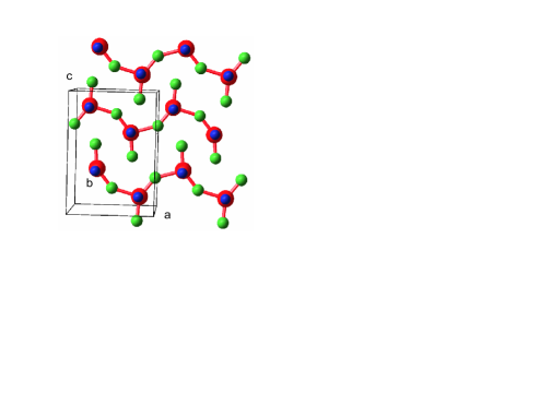
Figure 1: Position of the ${\rm Cu^{2+}}$ (red), ${\rm Cl^{-}}$ (green) and ${\rm O^{-}}$ (blue) in the crystal structure of CDC. The dominant superexchange interactions are via ${\rm Cu^{2+}}$-${\rm Cl^{-}}$- ${\rm Cu^{2+}}$ paths forming linear chains along the a-axis. The axes of the quasi-planar ${\rm CuCl_{2}O_{2}}$ groups alternates by $22^{\circ}$ along the chain direction, leading to a staggered gyromagnetic tensor ${\bf g}$.

The crystal symmetry also allows the presence of DM interactions Dzyaloshinskii (1958); Moriya (1960)

$${\mathcal{H}}_{\rm DM}=\sum_{n}{\bf D}_{n}\cdot({\bf S}_{n-1}\times{\bf S}_{n})\,.$$ (3)

The DM vector ${\bf D}_{n}=(-1)^{n}D{\bf{\hat{b}}}$ alternates from one chain site to the next as can be seen from the space group symmetry: First, the structure is invariant under a translation along the a-axis by two Cu sites, meaning that there can be at most two distinct DM vectors. Second, the ac plane is a mirror plane, implying that the DM vectors point along the b-axis. Third, the crystal structure is invariant under the combined operation of translation by one Cu site along the chain, and reflection in the ab-plane.

It was shown that alternating DM interactions can result in an effective staggered field ${\bf H_{\rm st}}$ upon application of a uniform external field ${\bf H}$ (Ref. Oshikawa and Affleck, 1997). Taking into account also the staggered ${\bf g}$ tensor, the effective staggered field that is generated by a uniform field can be written as

$${\bf g^{u}}{\bf H_{\rm st}}=\frac{1}{2J}{\bf D}\times{\bf g^{u}}{\bf H}+{\bf g^{s}}{\bf H}\,.$$ (4)

III Experimental Techniques

Single crystals of CDC were obtained by slow cooling from $T=50^{\rm o}\mathrm{C}$ to $20^{\rm o}\mathrm{C}$ of saturated methanol solutions of anhydrous $\mathrm{CuCl_{2}}$ and dimethyl sulphoxide in a 1:2 molar ratio. Emerald-green crystals grow as large tabular plates with well developed (001) faces. Specific heat measurements were performed on small, protonated crystals with a typical mass of $15\;\mathrm{mg}$ in a dilution refrigerator, using relaxation calorimetry in magnetic fields up to $9\;\mathrm{T}$ applied along the three principal crystallographic directions. Measurements were performed in six different magnetic fields applied along the a- and b-axes, and eight different fields applied along the c-axis.

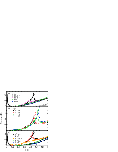
Figure 2: Specific heat of CDC as a function of temperature for magnetic field applied along the a, b and c-axis. The peaks in the temperature dependence correspond to the onset of long-range magnetic order. The solid (and the mostly hidden dashed) line corresponds to the low-temperature specific heat calculated in the framework of the sine-Gordon (boson) model and described in Eq. 10 (Eq. 6). Dotted line plotted in (a) corresponds to $aT^{3}$ lattice contribution to the specific heat.

Neutron diffraction measurements were performed on deuterated single crystals of mass $1\mathrm{g}$ using the SPINS spectrometer at the NIST Center for Neutron Research. Inelastic neutron scattering experiments were performed on multiple co-aligned single crystals with a total mass of $7.76\;\mathrm{g}$ using the DCS spectrometer at NIST. The SPINS spectrometer was configured with horizontal beam collimations $45^{\prime}/k_{i}\;{\rm(}^{58}{\rm Ni}\;{\rm guide)}-80^{\prime}-80^{\prime}-300^{\prime}$. A pyrolytic graphite (PG) monochromator was used to select incident neutron energies of either $E_{i}=3\;\mathrm{meV}$, $5\;\mathrm{meV}$ (using the $(0,0,2)$ reflection) or $20\;\mathrm{meV}$ (using the $(0,0,4)$ reflection). For $E_{i}=3\;\mathrm{meV}$ and $5\;\mathrm{meV}$ a cooled Be filter was used before the sample to eliminate contamination from higher-order monochromator Bragg reflections. The DCS measurements were performed with an incident energy $E_{i}$=$4.64\;\mathrm{meV}$ and an angle of $60^{o}$ between the incident beam and the a-axis, as detailed in Ref. Kenzelmann et al., 2004.

IV Specific heat measurements

The temperature dependence of the specific heat at low fields has a well-defined peak for all field directions, as shown in Fig. 2. The peak position varies with field strength and direction, all of which suggests that the peak corresponds to the onset of long-range magnetic order. At zero-field, the transition temperature is $T_{N}$=$0.93\;\mathrm{K}$, in agreement with prior zero-field heat capacity measurements.Flipsen When the field is applied in the mirror plane, either along the a or the c-axis, the ${\rm Ne\acute{e}l}$ temperature $T_{N}$ decreases with increasing field, as shown in Fig. 2(a) and Fig. 2(c). The peak becomes unobservable above $\mu_{0}H_{c}$=$5.7$ and $\mu_{0}H_{c}$=$3.9\;\mathrm{T}$ for fields applied along the a- and c-axis, respectively. At higher fields, the specific heat is exponentially activated, with spectral weight shifting to higher temperatures with increasing field. This is evidence for a spin gap for magnetic fields along the a- and c-axes. In contrast, a magnetic field along the b-axis enhances the magnetic order and the ${\rm Ne\acute{e}l}$ temperature increases with increasing field strength, as shown in Fig. 2(b).

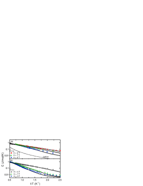
Figure 3: Semilogarithmic plot of the specific heat $C(H,T)$ in the high-field gapped phase as a function of the inverse temperature $1/T$ for different magnetic fields applied along the (a) a and (b) c-axes, respectively. The solid (dashed) line corresponds to the low-temperature specific heat calculated in the framework of the sine-Gordon (boson) model and given in Eq. 10 (Eq. 6). Dotted line plotted in (a) corresponds to $aT^{3}$ lattice contribution to the specific heat.

We analyze the specific heat for $H>H_{c}$ to determine the field dependence of the spin gap. The low-temperature specific heat is first compared to a simple model (which we refer to as the boson model) of ñ species of one-dimensional non-interacting gapped bosons with a dispersion relation

$${\hbar}{\omega}(\tilde{q})=\sqrt{\Delta^{2}+[v(\tilde{q}-{\tilde{q}}_{0})]^{2}}\,.$$ (5)

Here $\Delta$ is the spin gap, $v$ is the spin-wave velocity, which depends on both the strength and orientation of the magnetic field, ${\tilde{q}}$ is the chain wave-vector ${\tilde{q}}=\pi h$ and ${\tilde{q}}_{0}=\pi$. The specific heat of a one-dimensional boson gas in this boson model is given byTroyer et al. (1994)

$$C_{\rm mag}(T)=\frac{\tilde{n}R}{\sqrt{2\pi}}\left(\frac{\Delta}{k_{B}T}\right)^{\frac{3}{2}}\frac{\Delta}{v}\exp(-\Delta/k_{B}T)\,.$$ (6)

Terms proportional to $\frac{H^{2}}{T^{2}}$ and to $T^{3}$ were included in the fit to take into account the small nuclear spin and lattice contributions, respectively. The total function fitted to the specific heat was

$$C(T,H)=C_{\rm mag}+aT^{3}+b(H/T)^{2}\,.$$ (7)

All data for $T<\Delta$ and $H>H_{c}$ were fit simultaneously to Eq. 7, yielding $a=0.027(1)\;\mathrm{J/molK^{4}}$ and $b=8(2)\cdot 10^{-6}\;\mathrm{JmolK/T^{2}}$. The average spin-wave velocity is found to be $v/\tilde{n}=0.65(1)$ and $0.58(2)\;\mathrm{meV/mode}$ for fields along the a- and c-axis, respectively. From our previous measurements of the field-induced incommensurate mode Kenzelmann et al. (2005) we found that the spin-wave velocity is $v=1.84(4)\;\mathrm{meV}$. This yields $\tilde{n}=2.8$ for the number of gapped low-energy modes which contribute to the specific heat, in excellent agreement with the expectation of one longitudinal and two transverse modes. The resulting field and orientation dependent spin gaps are shown in Fig. 4, and the calculated $C(T,H)$ for the boson model are plotted as dashed lines in Figs. 2 and 3.

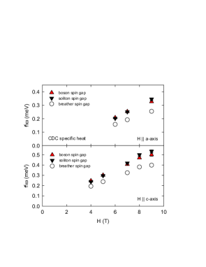
Figure 4: Field dependence of the energy gaps for the boson and sine-Gordon models, derived from fits to specific heat data as shown in Fig. 3. The error bars are smaller than the symbol size.

We also analyze the specific heat in the framework of the sine-Gordon model, to which the Hamiltonian can be mapped in the long wave-length limit Oshikawa and Affleck (1997). The sine-Gordon model is exactly solvable, with solutions that include massive soliton and breather excitations. The soliton mass, $M$, is given byDashen et al. (1975); Affleck and Oshikawa (1999)

$$M\approx J(\frac{g\mu_{B}H_{\rm st}}{J})^{(1+\xi)/2}$$

$$\{B(\frac{J}{g\mu_{B}H})^{(2\pi-\beta^{2})/4\pi}(2-\frac{\beta^{2}}{\pi})^{1/4}\}^{-(1+\xi)/2}.$$ (8)

Here $\xi=\beta^{2}/(8\pi-\beta^{2})\rightarrow 1/3$ for $\mu_{0}H\rightarrow 0$, $B=0.422169$, and $\mu_{0}H_{\rm st}$ is the effective staggered field. The mass of the breathers, $M_{n}$, is given by

$$M_{n}=2M\sin(n\pi\xi/2)\,,$$ (9)

where $1\leq n\leq[1/\xi]$ with $\xi$ depending entirely on the applied field Essler and Tsvelik (1998). The temperature dependence of the specific heat due to breathers and solitons is given by

$$C\sim\sum_{\alpha=0}^{[1/\xi]}\frac{(1+\delta_{\alpha 0})M_{\alpha}}{\sqrt{2\pi}v}\left[1+\frac{k_{B}T}{M_{\alpha}}+\frac{3}{4}\left(\frac{k_{B}T}{M_{\alpha}}\right)^{2}\right]$$

$$\cdot\left(\frac{M_{\alpha}}{k_{B}T}\right)^{\frac{3}{2}}\exp\left(-\frac{M_{\alpha}}{k_{B}T}\right)\,,$$ (10)

where $M_{0}\equiv M$. We use this expression for an additional comparison to the experimentally-observed temperature and field dependence of the specific heat $C(T,H)$ for $T<M_{1}$ and $H>H_{c}$, in order to determine the soliton mass as a function of field strength and orientation. These results are shown as solid lines in Figs. 2 and 3. The adjusted soliton and breathers masses are shown in Fig. 4, in comparison with the results from the boson model.

The adjusted boson mass is larger than the breather mass, but smaller than the soliton mass, as expected from a model which is only sensitive to an average gap energy. The soliton energy is different for fields applied along the a- and c-axis as a result of different staggered fields arising from the staggered $g$-factor and DM interactions.

The field dependence of the gap for two different field directions allows an estimate of the strength of $g_{s}$ and $D/J$. The best estimate is obtained for high fields where the effect of the low-field ordered phase is small. Assuming $H_{\rm st}=cH$ and fitting Eq. 8 to the field dependence of the gap, we obtain $c=0.045(2)$ for fields along the a-axis and $c=0.090(4)$ for fields along the c-axis. Comparing these results with Eq. 4 we obtain

$$g^{s}-g^{aa}D/2J=0.045$$

$$g^{s}+g^{cc}D/2J=0.09\,.$$ (11)

With $g^{aa}=2.28$ and $g^{cc}=2.12$ (Ref. Landee et al., 1987), this leads to $g^{s}=0.068(3)$ and $D/J=0.0102(5)$, establishing the presence of both sizeable DM interactions and a staggered $g$ factor in CDC.

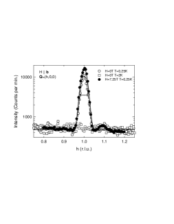
Figure 5: (h,0,0) scans through ${\bf Q}=(1,0,0)$ magnetic Bragg peak in CDC at $T=0.25$K, $\mu_{0}H=7.25$ T$||{\bf b}$, $T=0.25$K and $T=2$K at zero field. The bar in the figure represents the calculated peak width of ${\bf Q}=(1,0,0)$ based on the known instrumental resolution. The peak at $h=1.09$ appears to be field and temperature independent indicating that it does not arise from magnetic scattering.

V Neutron diffraction

Neutron diffraction measurements were performed in the $(h,0,l)$ and $(h,k,0)$ reciprocal lattice planes. Fig. 5 shows $h$-scans through the $(1,0,0)$ reflection for different temperatures and fields. At zero field and $T=0.3\;\mathrm{K}$ a resolution-limited peak is observed at $h=1$. The peak is absent for temperatures higher than $T_{N}=0.93\;\mathrm{K}$. No incommensurate order was observed in any of our experiments. The reflections we found can be indexed by $(2\cdot n,m,0)$ in the $(h,k,0)$ plane, whereas magnetic diffraction was found only at the $(1,0,0)$ and the $(3,0,0)$ reciprocal lattice points in the $(h,0,l)$ plane for $|{\bf Q}|<2.6\AA^{-1}$.

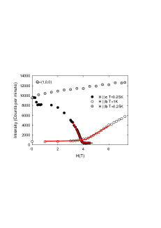
Figure 6: Measured field dependence of the ${\bf Q}=(1,0,0)$ magnetic peak intensity at $T=0.25\;\mathrm{K}$ with the field applied along the c-axis and at $T=0.25$K and at $T=1\;\mathrm{K}$ with the field applied along the b-axis. The solid lines represent the fits explained in Sect. V.3.

V.1 HT-Phase Diagram

The phase diagram of CDC was further explored with neutron diffraction for fields up to $7.25\;\mathrm{T}$, applied along the b and c-axis. Figure 6 summarizes the magnetic field dependence of elastic scattering measurements at the $(1,0,0)$ wave-vector. Applying a field along the b-axis increases the intensity of the $(1,0,0)$ reflection and we associate this with an increase in the staggered magnetization. In contrast, a field along the c-axis decreases the intensity of the $(1,0,0)$ Bragg peak, first in a sharp drop at $0.3\;\mathrm{T}$ suggestive of a spin-flop transition, and then in a continuous decrease towards a second phase transition at $3.9\;\mathrm{T}$. The transition at $3.9\;\mathrm{T}$ is evidence that exchange-induced long-range order is suppressed by the application of fields along the c-axis. The value of the critical field, $3.9\;\mathrm{T}$, is in agreement with specific heat measurements.

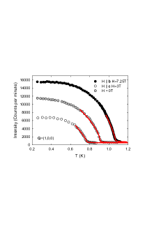
Figure 7: Measured temperature dependence of the ${\bf Q}=(1,0,0)$ magnetic peak intensity for zero field, $\mu_{0}H=7.25\;\mathrm{T}$ applied parallel to the b-axis and $\mu_{0}H=3\;\mathrm{T}$ applied parallel to the c-axis. The solid lines represent the fits explained in Sect. V.3.

Fig. 7 shows the temperature dependence of the $(1,0,0)$ magnetic Bragg peak for fields applied along the b- and c-axis. For fields along the b-axis, the Bragg peak has higher intensity at low T and the enhanced intensity survives to higher temperatures than in the zero field measurement. For fields along the c-axis, the intensity is reduced and the transition temperature is lower than at zero field. The phase transition remains continuous, regardless of the direction of the field.

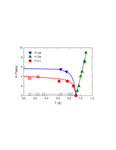
Figure 8: Field-temperature phase diagram of CDC determined from heat capacity measurements (filled symbols) and from neutron scattering (open symbols). The squares indicate the spin-flop transition observed for a field along the c-axis. The solid and dashed lines are a guide to the eye.

The phase diagram in Fig. 8 shows a synopsis of the results obtained from specific heat and neutron diffraction measurements. CDC adopts long-range magnetic order below $T_{N}$. This order can be strengthened by the application of a magnetic field along the b-axis, which enhances the ordered moment and increases the transition temperature to long-range order. In contrast, applying fields along the a- and c-axes competes with the zero-field long-range order, decreases the critical temperature leading eventually to the collapse of the low-field long-range order at $5.9$ and $3.9\;\mathrm{T}$ respectively, as extrapolated to zero temperature.

V.2 Magnetic Structures

To understand the field-induced phase transitions, it is important to determine the symmetry of the magnetic structures below and above the transitions. The intensities of $\sim 40$ magnetic Bragg peaks were measured at $0.1\;\mathrm{K}$ at zero field, at $\mu_{0}H=0.5\;\mathrm{T}$ and at $10\;\mathrm{T}$ applied along the c-axis. The ordering wave-vector for both structures is ${\bf k}=(0,0,0)$. We use group theory to identify the spin configurations consistent with the wave-vector ${\bf k}$ for the given crystal symmetry, and compare the

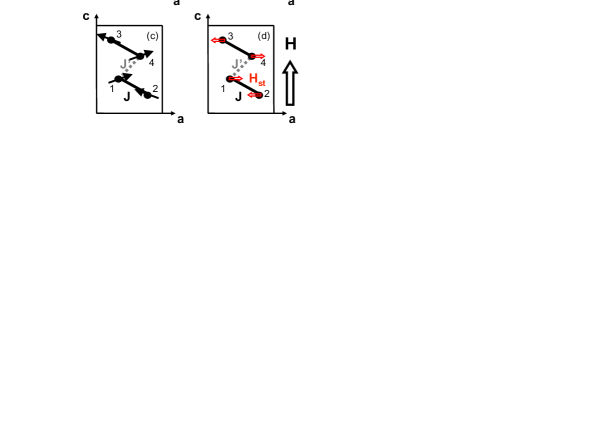
Figure 9: Magnetic structures at zero field (a), $0.75\;\mathrm{T}$ (b) and $10\;\mathrm{T}$ (c), with the field ${\rm H}$ applied along the c-axis. The solid arrows indicate the spin directions, + and - indicate spins pointing into opposite directions along the b-axis. The ${\rm Cu^{2+}}$ positions are defined in Appendix A. Because the ordering wave-vector is ${\bf k}=(0,0,0)$, the spin arrangement in other unit cells is identical. (d) Directions of the staggered fields ${\bf H_{\rm st}}$ upon application of an external field ${\bf H}$ along the c-axis.

structure factor of possible spin configurations with the observed magnetic Bragg peak intensities. The group theoretical analysis which leads to the determination of the symmetry-allowed basis vectors is presented in Appendix B.

At zero field and $T=0.1\;\mathrm{K}$, best agreement (see Table 1 and Fig. 10a-b) with the experiment is obtained for a magnetic structure belonging to representation $\Gamma^{2}$ as defined in Appendix B with $\chi^{2}=3.1$ and $R=0.43$. The magnetic structure is collinear with a moment of $0.44(5)\mu_{B}$ along the c-axis as shown in Fig. 9(a). The alignment of the moment along the c-axis suggests an easy-axis anisotropy along this direction, which is not included in the zero-field Hamiltonian defined by Eq. 1. The ordered magnetic moment is significantly less than the free-ion moment, as expected for a system of weakly-coupled $S=\frac{1}{2}$ chains close to a quantum critical point Schulz (1996).

	($h$,$k$,$l$)	$I_{\rm exp}$	$I_{\rm cal}$
	( -1, 7, 0)	-4 (2)	1.38
	( -1, 8, 0)	0 (2)	3.43
	( 0, 3, 0)	0 (2)	0
	( 0, 7, 0)	0 (2)	0
	( 3, 4, 0)	1 (2)	0.722
	( 3, 2, 0)	3 (2)	1.12
	( 5, 1, 0)	3 (2)	4.17
	( 3, 5, 0)	4 (2)	9.11
	( 5, 2, 0)	5 (2)	2.21
	( 3, 7, 0)	5 (2)	3.7
	( 3, 6, 0)	5 (2)	0.344
	( -1, 5, 0)	5 (2)	3.32
	( 5, 3, 0)	5 (2)	3.09
	( 1, 8, 0)	5 (2)	3.43
	( 1, 7, 0)	5 (2)	1.38
	( 1, 5, 0)	5 (2)	3.32
	( 1, 3, 0)	6 (2)	6.55
	( 5, -1, 0)	7 (2)	4.17
	( -1, 6, 0)	7 (2)	9.76
	( -1, 3, 0)	8 (2)	6.55
	( 1, 6, 0)	8 (2)	9.76
	( 5, 0, 0)	11 (2)	2.57

Table 1: Measured magnetic Bragg peak intensities at $\mu_{0}H=0\;\mathrm{T}$, compared with the best fit with $\chi^{2}=3.1$ and $R=0.43$. The found magnetic structure belongs to $\Gamma^{2}$ and the moment is aligned along the z-axis. The next best fit yields a magnetic structure that belongs to $\Gamma^{5}$ with the magnetic moments aligned along the y-axis, with $\chi^{2}=5.2$ and $R=0.67$.

At $\mu_{0}H=0.75\;\mathrm{T}$ after the system undergoes a spin-flop transition, the magnetic order can be described by the representation $\Gamma^{5}$ with $\chi^{2}=1.75$ and $R=0.49$ ( Table 2 and Fig. 10c) . Slightly lower values for $\chi^{2}$ are obtained if a small antiferromagnetic moment belonging to $\Gamma^{8}$ is also allowed for. As shown in Fig. 9(b), the spin structure is collinear with a magnetic moment of $0.3(1)\mu_{B}$ per ${\rm Cu^{2+}}$ along the b-axis (and perpendicular to the field as expected for a spin-flop transition).

	($h$,$k$,$l$)	$I_{\rm exp}$	$I_{\rm cal}$
	( 1, 5, 0)	-1 (1)	0.321
	( 5, 1, 0)	0 (1)	5.05
	( 1, 7, 0)	0 (1)	0.0705
	( 1, 6, 0)	0 (1)	0.671
	( 1, 3, 0)	0 (1)	1.54
	( 0, 3, 0)	0 (2)	0
	( 0, 7, 0)	0 (2)	0
	( 3, 4, 0)	0 (1)	0.485
	( 3, 2, 0)	0 (1)	1.15
	( 3, 7, 0)	1 (2)	1.28
	( 1, 8, 0)	1 (1)	0.136
	( 3, 6, 0)	2 (2)	0.147
	( 3, 5, 0)	2 (2)	4.87
	( 5, 2, 0)	2 (2)	2.54
	( 5, 3, 0)	4 (2)	3.26
	( 5, 0, 0)	4 (2)	3.17

Table 2: Measured magnetic Bragg peak intensities at $\mu_{0}H=0.75\;\mathrm{T}$, compared with the best fit with $\chi^{2}=1.75$ and $R=0.49$. The found magnetic structure belongs to $\Gamma^{5}$ and the moment is aligned along the y-axis. The next best fit yields a magnetic structure that belongs to $\Gamma^{4}$ with the magnetic moments aligned along the x-axis, with $\chi^{2}=5.3$ and $R=0.96$.

At $\mu_{0}H=10\;\mathrm{T}$, the magnetic order can be described by representation $\Gamma^{8}$ with $\chi^{2}=2.41$ and $R=0.21$ ( Table 3 and Fig. 10) . The spin structure is a collinear magnetic structure where the magnetic moments point along the a-axis, perpendicular to the external field and along the staggered fields in the material, as shown in Fig. 9(c). The antiferromagnetically ordered moment along the a-axis is $0.49(5)\mu_{B}$ per ${\rm Cu^{2+}}$. Our numerical calculations Kenzelmann et al. (2005) using a the Lanczos method for finite chains of 24 sites yield a ordered staggered moment $0.55\mu_{B}$ per site, in good agreement with the experiment.

The magnetic structures reveal why fields along the a- and c-axis lead to the collapse of long-range order, while a field along the b-axis strengthens magnetic order. A field along the c-axis leads to staggered fields due to the alternating $g$ tensor and DM interactions, as illustrated in Fig. 9(d). These staggered fields compete with inter-chain interactions which favor a different antiferromagnetic arrangement of spins. For example, inter-chain exchange favors AF alignment of the neighboring magnetic moments on sites 1 and 4, but the staggered fields favor ferromagnetic alignment along the a-axis. This must lead to an increase in quantum fluctuations which leads to a collapse of magnetic order, identifying the transition as a quantum phase transition. This situation was recently analyzed in great detail by Sato and Oshikawa.Sato and Oshikawa (2004).

	($h$,$k$,$l$)	$I_{\rm exp}$	$I_{\rm cal}$
	( 5, 1, 0)	-5 (2)	0.0479
	( 5, 0, 0)	-3 (2)	0
	( 5, -1, 0)	-2 (2)	0.0479
	( 3, 5, 0)	-1 (2)	0.308
	( 3, 7, 0)	-1 (2)	0.159
	( 5, 3, 0)	-1 (2)	0.278
	( 5, 2, 0)	0 (2)	0.273
	( 0, 3, 0)	0 (2)	0
	( 0, 7, 0)	0 (2)	0
	( -1, 7, 0)	0 (2)	6.05
	( -1, 8, 0)	1 (2)	0.792
	( 1, 8, 0)	2 (2)	0.792
	( 1, 6, 0)	2 (2)	22
	( -1, 6, 0)	2 (2)	22
	( 3, 2, 0)	4 (2)	3.57
	( 3, 6, 0)	6 (2)	4.13
	( 3, 4, 0)	7 (2)	6.04
	( 1, 7, 0)	8 (2)	6.05
	( -1, 5, 0)	14 (2)	14
	( 1, 5, 0)	20 (2)	14
	( -1, 3, 0)	21 (2)	24.3
	( 1, 3, 0)	23 (2)	24.3

Table 3: Measured magnetic Bragg peak intensities at $\mu_{0}H=10\;\mathrm{T}$, compared with the best fit with $\chi^{2}=2.4$ and $R=0.21$. The found magnetic structure belongs to $\Gamma^{8}$ and the moment is aligned along the x-axis. The next best fit yields a magnetic structure that belongs to $\Gamma^{6}$ with the magnetic moments aligned along the z-axis, with $\chi^{2}=8.2$ and $R=0.34$.

Application of a field along the b-axis does not induce staggered fields, and so merely quenches quantum fluctuations for small field strengths, thereby leading to an enhancement of the antiferromagnetically ordered moment as observed in the experiment. Application of a field along the a-axis should not lead to a spin-flop transition, because the moments in the zero-field structure are already perpendicular to that field direction. At higher fields, however, the competition between magnetic order arising from either spin exchange or staggered fields becomes important, leading eventually to the phase transition at $\mu_{0}H=5.7\;\mathrm{T}$ into a gapped phase that is described by the sine-Gordon model.

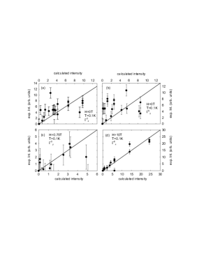
Figure 10: (a-d) Observed magnetic intensities plotted as a function of calculated intensities, showing the quality of our fits. (a-b) compares the best fit for $\mu_{0}H=0\;\mathrm{T}$ with the second best fit, while (c-d) show the best fits for $\mu_{0}H=0.75\;\mathrm{T}$ and $\mu_{0}H=10\;\mathrm{T}$, respectively.

V.3 Critical Exponents

The neutron diffraction measurements allow determination of the order parameter critical exponent $\beta$ for the phase transition to long-range order. Fig. 11 shows the magnetic intensity of the $(1,0,0)$ reflection close to the critical region. The data were corrected for a non-magnetic, constant background.

The temperature scans are shown as a function of reduced temperature $(1-T/T_{c})$ for zero field, $\mu_{0}H=7.25\;\mathrm{T}$ applied along the b-axis and $\mu_{0}H=3\;\mathrm{T}$ applied along the c-axis. Power law fits were performed using

$$I(H)\propto|T-T_{N}|^{2\beta}\,.$$ (12)

It was found that $\beta=0.30(1)$ for zero field, $\beta=0.35(1)$ for $\mu_{0}H=7.25\;\mathrm{T}$ and $\beta=0.36(1)$ for $\mu_{0}H=3\;\mathrm{T}$. Fits were performed over a reduced temperature of $0.2$.

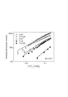
Figure 11: Logarithmic plot of the background corrected ${\bf Q}=(1,0,0)$ magnetic intensity plotted as a function of reduced temperature (open symbols) or versus reduced field (filled symbols). Dashed lines corresponds to the power law fits described in the text. For the temperature scans, $\mu_{0}H=7.25\;\mathrm{T}$ was applied along the b-axis, and $\mu_{0}H=3\;\mathrm{T}$ was applied along the c-axis. For the field scans at constant temperature, the field was applied along the b-axis for $T=1\;\mathrm{K}$ and along the c-axis for $T=0.25\;\mathrm{K}$.

Figure 11 also shows two field scans: one scan with the field applied along the c-axis and performed at $0.25\;\mathrm{K}$, and a scan with the field applied along the b-axis, performed at $1\;\mathrm{K}$. The latter transition is unlike all other transitions discussed here, because here the field induces an ordered state starting from a paramagnetic state. The field scans are shown as a function of reduced field $|1-H/H_{c}|$. Power law fits were made using

$$I(T)\propto|H-H_{c}|^{2\beta}$$ (13)

in order to determine the critical exponents and it was found that $\beta=0.400(1)$ for $T=0.25\;\mathrm{K}$ and $\beta=0.481(3)$ for $T=1\;\mathrm{K}$. Fits were performed over the range $0.2$ in reduced field.

For the temperature driven transition, the critical exponents $\beta$ fall in the range $0.30\sim 0.36$ depending on the direction of the applied field, consistent with the critical exponents of three-dimensional Ising universality class,LeGuillou and Zinn-Justin (1980) to which CDC belongs at zero field. For the field-induced transitions, the Ising character of the spin symmetry is enhanced due to the presence of a uniform and perpendicular staggered field. The critical exponent for the field-induced transitions, $\beta=0.400(1)$ and $\beta=0.481(3)$, are however higher than the critical exponent $\beta=0.325$ of the three-dimensional Ising universality class.

For an Ising quantum phase transition ($T=0$), the effective dimension of the quantum critical point is $D=d+z$ where $d=3$ is the spatial dimension and $z=1$ is the dynamical exponent. Since $D=4$ is the upper critical dimension, the quantum critical point is Gaussian (with logarithmic corrections) and $\beta=0.5$. Therefore, by measuring the field dependence of the order parameter at different temperatures, we expect to observe a crossover between the classical (finite $T$ and $\beta=0.325$) and the quantum phase transitions ($T=0$ and $\beta=0.5$). This seems to be the natural explanation for the observed values of $\beta$ close to $0.5$. A similar increase in the apparent $\beta$ critical exponent was observed in the singlet ground state system PHCC.Stone et al. (2006)

VI Inelastic Neutron Scattering

VI.1 Exchange Interactions

To characterize the Hamiltonian and accurately determine the strength of the spin interaction along the chain, we performed an energy scan for wave-vector transfer ${\bf Q}\cdot{\bf a}=\pi$ along the chain. At this wave-vector the two-spinon spectrum characteristic of the AF $S=\frac{1}{2}$ chain should be concentrated over a small energy window and form a well-defined peak located at $\hbar\omega=\pi J/2$. Fig. 12 shows that this is indeed the case, and that for CDC this well-defined excitation is located at $\hbar\omega=2.43(2)\;\mathrm{meV}$. A fit to the exact two-spinon cross-section Bougourzi et al. (1998) convolved with the experimental resolution yields an excellent description of the observed spectrum, as shown in Fig. 12 for a value of intra-chain exchange $J=1.46(1)\;\mathrm{meV}$. This value is very similar to that obtained from the temperature dependence of the magnetic susceptibility, which was $1.43\;\mathrm{meV}$.Landee et al. (1987)

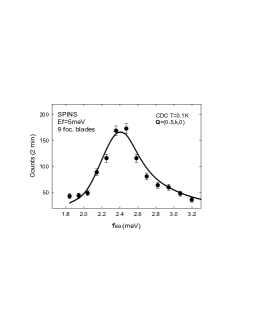
Figure 12: Neutron scattering intensity as a function of energy transfer for zero-field for $h=0.5$ measured using SPINS. The measurement was performed with $9$ analyzer blade channels set to reflect $E_{f}=5\;\mathrm{meV}$ to the center of the detector. A Be filter rejected neutrons with energies higher than $5\;\mathrm{meV}$ from the detection system. The measurements were performed with the strongly dispersive direction along the scattered neutron direction, so that the measurements integrate neutron scattering over wave-vectors along a weakly-dispersive direction. The solid line represents the exact two-spinon cross-section Bougourzi et al. (1998) for $J=1.46(1)\;\mathrm{meV}$, convolved with the experimental resolution.

VI.2 Ground state energy at zero field and $\mu_{0}H=11\;\mathrm{T}$

Inelastic neutron scattering not only allows determination of exchange constants, but also a measurement of the ground state energy. The expectation value of the Hamiltonian, $<{\mathcal{H}}>$, is proportional to the first moment of the dynamic structure factor, defined as $\langle\tilde{\omega}\rangle_{{\bf Q}}=\hbar^{2}\int d\omega\omega S({\bf Q},\omega)$. Here the normalization of $S({\bf Q},\omega)$ is chosen such that the total moment sum rule reads: $\hbar\int S({\bf Q},\omega)d\omega=S(S+1)/3$. So if the dynamic structure factor, $S({\bf Q},\omega)$, is measured in absolute units, neutron scattering yields a measurement of $<{\mathcal{H}}>$ as a function of field or temperature.

For a Heisenberg AF chain, the wave-vector dependence of $\langle\tilde{\omega}\rangle_{h}$ is given by

$$\langle\tilde{\omega}\rangle_{h}=-\frac{2}{3}<{\mathcal{H}}>(1-\cos(\pi h))\,.$$ (14)

We use this relation to describe the measured first moment, $\langle\tilde{\omega}\rangle_{h}$. Figure 13 shows that at zero field the experimental $\langle\tilde{\omega}\rangle_{h}$ follows this expression with $<{\mathcal{H}}>=-0.4(1)J$ - in excellent agreement with Bethe’s result of $<{\mathcal{H}}>\simeq-0.44J$ (Ref. Bethe, 1931). $\langle\tilde{\omega}\rangle_{h}$ was obtained by fitting the exact two-spinon cross-section $S_{\rm 2sp}({\bf Q},\omega)$ as calculated by Bougourzi et al.Bougourzi et al. (1998) to the data and computing $\langle\tilde{\omega}\rangle_{h}$ from the analytical expression for $S_{\rm 2sp}({\bf Q},\omega)$.

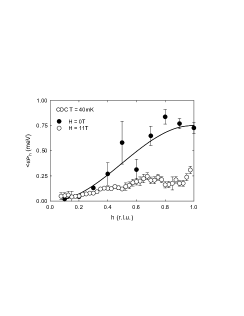
Figure 13: First moment $\langle\tilde{\omega}\rangle_{h}=\hbar^{2}\int d\omega\omega I(h,\omega)$ of the well-defined excitations only as a function of wave-vector $h$ along the chain, for zero field and $\mu_{0}H$=$11\;\mathrm{T}$. The raw scattering data were corrected for a time-independent background measured at negative energy transfer, for monitor efficiency, and for the ${\rm Cu^{2+}}$ magnetic form factor, folded into the first Brillouin zone, and put onto an absolute scale using the elastic incoherent scattering from CDC.

Fig. 13 shows the first moment $\langle\tilde{\omega}\rangle_{h}$ at $\mu_{0}H=11\;\mathrm{T}$ including contributions only from sharp modes in the spectrum, thus excluding any contributions from continuum scattering. It was calculated by fitting a Gaussian to the experimentally observed peak in the energy spectra and by integrating the area under the Gaussian curve. $\langle\tilde{\omega}\rangle_{h}$ at $\mu_{0}H=11\;\mathrm{T}$ is generally about $3$ times smaller than $\langle\tilde{\omega}\rangle_{h}$ at zero field. This is evidence for the presence of substantial magnetic continuum scattering because both numerical and analytical calculations show that the first moments in an applied magnetic field should be larger than this measured value. This is based upon (A) numerical calculations Kenzelmann et al. (2005) using the Lanczos method for finite chains of length between 12 and 24 spins which show that the ground state energy at $\mu_{0}H=11\;\mathrm{T}$ for $H_{\rm st}=0.075H$ is $<{\mathcal{H}}>=-0.34J$, and (B) analytical calculations of the field dependence of the first moment which show that Eq. 14 acquires merely a small constant value with the application of uniform and staggered fields. Points (A) and (B) thus show that theoretically, only a slight depression of the first moment is expected upon application of magnetic fields.

Because our data presented in Fig. 13 include only resonant modes this result indicates that there are substantial contributions to the first moment from continuum scattering - perhaps not a surprise given that continuum scattering is the sole source of the first moment at zero field.

VI.3 Comparison with the chains-MF model

The magnetic order of weakly-coupled chains can be described by a chain mean-field theory developed by Schulz Schulz (1996). It gives the following relations between ordered magnetic moment $m_{0}$, $T_{N}$ and the average of inter-chain interactions $|J^{\prime}|$:

$$|J^{\prime}|=\frac{T_{N}}{1.28\sqrt{\ln(5.8J/T_{N})}}$$ (15)

$$m_{0}=1.017\sqrt{|J^{\prime}|/J}\,.$$ (16)

The first relation allows an estimate for $|J^{\prime}|$. In our case, where $T_{N}=0.93\;\mathrm{K}$ and $J=1.5\;\mathrm{meV}$, this gives $|J^{\prime}|=0.03\;\mathrm{meV}$. The real value for $|J^{\prime}|$ may be somewhat higher because quantum fluctuations are not fully accounted for in the chain mean-field theory.

The second relation predicts the ordered moment for a Heisenberg chain magnet $m_{0}=0.14\;\mu_{B}$ for $|J^{\prime}|=0.03\;\mathrm{meV}$, which is considerably lower than the observed ordered moment even if one considers a higher value for $|J^{\prime}|$ due to quantum fluctuations. The large discrepancy may be due to the Ising-type spin anisotropy which fixes the zero-field ordered moment along the c-axis, thereby quenching quantum fluctuations and enhancing long-range order at low temperatures. Indeed, this term, no matter how small, induces long-range order even in the purely 1D model at $T=0\;\mathrm{K}$.

VII Conclusions

CDC is a rich model system in which to study quantum magnetism because an applied magnetic field leads first to a first-order phase transition and then to a novel high-field phase with soliton excitations via a quantum critical phase transition. In this paper, we characterized the material and its proximity to quantum criticality using specific heat and neutron scattering measurements. We determined the phase diagram as a function of temperature and field applied along all three crystallographic directions. The Bragg peak intensities and the temperature dependence of the specific heat demonstrate that when applying a field along the a- and c-axes, the spin system undergoes a quantum phase transition due to competing magnetic order parameters. Beyond the critical field, specific heat measurements show activated behavior typical for a gapped excitation spectrum. Theoretical analysis indicates that the spin gap results from spinon binding due to a staggered gyromagnetic factor and DM interactions. The gap energy was extracted from specific heat data using both a non-interacting boson model and an expression derived from a mapping of the Hamiltonian to the sine-Gordon model. We determined the strength of the staggered gyromagnetic factor and the DM interactions by analyzing the different field dependence of the gap for fields along the a- and c-axes. A magnetic field along the c-axis leads to two phase transitions: a first-order spin-flop transition and a continuous phase transition at higher field to magnetic order described by only one irreducible representation. The continuous field driven quantum phase transition was characterized by an apparent critical exponent $\beta$, which is higher than expected for a classical phase transition in a 3D antiferromagnet. The interpretation of this result is that the experiment probes a cross over regime affected by the $T=0$ quantum critical transition, which is above its upper critical dimension and therefore mean field like.

VIII ACKNOWLEDGEMENTS

We thank C. Landee, J. Copley, I. Affleck, and F. Essler for helpful discussions, and J. H. Chung for help during one of the experiments. Work at JHU was supported by the NSF through DMR-9801742 and DMR-0306940. DCS and the high-field magnet at NIST were supported in part by the NSF through DMR-0086210 and DMR-9704257. ORNL is managed for the US DOE by UT-Battelle Inc. under contract DE-AC05-00OR2272. This work was also supported by the Swiss National Science Foundation under Contract No. PP002-102831.

Appendix A Definition of the magnetic sub-lattice in CDC

The unit cell contains four ${\rm Cu^{2+}}$ sites, which occupy the $4c$ position in the Pnma space group and are given by:

$${\bf r}_{1}=(0.3209,0.25,0.3614)$$

$${\bf r}_{2}=(0.8209,0.25,0.1386)$$

$${\bf r}_{3}=(0.1791,0.75,0.8614)$$

$${\bf r}_{4}=(0.6791,0.75,0.6386)$$ (17)

This numbering of the ${\rm Cu^{2+}}$ positions is used throughout the paper.

Appendix B Magnetic group theory analysis

Magnetic structures were inferred from diffraction data by considering only spin structures ”allowed” by the space group and the given ordering wave-vector ${\bf k}=(0,0,0)$. Landau theory of continuous phase transitions implies that a spin structure transforms according to an irreducible representation of the little group $G_{{\bf k}}$ of symmetry operations that leave the wave-vectors ${\bf k}$ invariant. The eigenvectors $\phi^{\lambda}$ of the $\lambda$-th irreducible representations $\Gamma^{\lambda}$ were determined using the projector method.Heine (1993) They are given by

$$\phi^{\lambda}=\sum_{g}\chi^{\lambda}(g)g(\phi)\,,$$ (18)

where $g$ is an element of the little group and $\phi$ is any vector of the order parameter space. $\chi^{\lambda}(g)$ is the character of symmetry element g in representation $\Gamma^{\lambda}$.

We start by considering the symmetry elements of the Pmna space group of CDC:

$$\{1,\;\overline{1},\;2_{x},\;2_{y},\;2_{z},\;m_{xy},\;m_{xz},\;m_{yz}\}\,.$$ (19)

Here $1$ is the identity operator, $\overline{1}$ is inversion at the origin, $2_{\alpha}$ denotes a 180^∘ screw axis along the crystallographic direction $\alpha=a,b$ or $c$ (180^∘ rotation operation followed by a translation). $m_{\alpha\beta}$ is a glide plane containing axes $\alpha$ and $\beta$. The group is nonsymmorphic because the group elements $\{R|{\bf a}\}$ consist of an operation $R$ followed by a translation ${\bf a}$ equal to half a direct lattice vector.

The ordering wave-vector ${\bf k}=(0,0,0)$ is invariant under all operations of the space group, so the little group $G_{\bf k}$ equals the space group. The group consists of $8$ different classes and therefore has $8$ irreducible representations. The irreducible representations and their basis vectors are given in Table 4. The magnetic representation can be written as

$$\Gamma^{k}=\Gamma^{1}\oplus 2\,\Gamma^{2}\oplus\Gamma^{3}\oplus 2\,\Gamma^{4}$$

$$\oplus\Gamma^{5}\oplus 2\,\Gamma^{6}\oplus\Gamma^{7}\oplus 2\,\Gamma^{8}\,.$$ (20)

	$\psi_{1}$	$\psi_{2}$	$\psi_{3}$	$\psi_{4}$	$\psi_{5}$	$\psi_{6}$	$\psi_{7}$	$\psi_{8}$
${\bf m}^{1}$	$\begin{array}[]{c}0\\ m_{y}\\ 0\end{array}$	$\begin{array}[]{c}m_{x}\\ 0\\ m_{z}\end{array}$	$\begin{array}[]{c}0\\ m_{y}\\ 0\end{array}$	$\begin{array}[]{c}m_{x}\\ 0\\ m_{z}\end{array}$	$\begin{array}[]{c}0\\ m_{y}\\ 0\end{array}$	$\begin{array}[]{c}m_{x}\\ 0\\ m_{z}\end{array}$	$\begin{array}[]{c}0\\ m_{y}\\ 0\end{array}$	$\begin{array}[]{c}m_{x}\\ 0\\ m_{z}\end{array}$
${\bf m}^{2}$	$\begin{array}[]{c}0\\ -m_{y}\\ 0\end{array}$	$\begin{array}[]{c}m_{x}\\ 0\\ -m_{z}\end{array}$	$\begin{array}[]{c}0\\ m_{y}\\ 0\end{array}$	$\begin{array}[]{c}-m_{x}\\ 0\\ m_{z}\end{array}$	$\begin{array}[]{c}0\\ -m_{y}\\ 0\end{array}$	$\begin{array}[]{c}m_{x}\\ 0\\ -m_{z}\end{array}$	$\begin{array}[]{c}0\\ m_{y}\\ 0\end{array}$	$\begin{array}[]{c}-m_{x}\\ 0\\ m_{z}\end{array}$
${\bf m}^{3}$	$\begin{array}[]{c}0\\ -m_{y}\\ 0\end{array}$	$\begin{array}[]{c}-m_{x}\\ 0\\ m_{z}\end{array}$	$\begin{array}[]{c}0\\ m_{y}\\ 0\end{array}$	$\begin{array}[]{c}m_{x}\\ 0\\ -m_{z}\end{array}$	$\begin{array}[]{c}0\\ m_{y}\\ 0\end{array}$	$\begin{array}[]{c}m_{x}\\ 0\\ -m_{z}\end{array}$	$\begin{array}[]{c}0\\ -m_{y}\\ 0\end{array}$	$\begin{array}[]{c}-m_{x}\\ 0\\ m_{z}\end{array}$
${\bf m}^{4}$	$\begin{array}[]{c}0\\ m_{y}\\ 0\end{array}$	$\begin{array}[]{c}-m_{x}\\ 0\\ -m_{z}\end{array}$	$\begin{array}[]{c}0\\ m_{y}\\ 0\end{array}$	$\begin{array}[]{c}-m_{x}\\ 0\\ -m_{z}\end{array}$	$\begin{array}[]{c}0\\ -m_{y}\\ 0\end{array}$	$\begin{array}[]{c}m_{x}\\ 0\\ m_{z}\end{array}$	$\begin{array}[]{c}0\\ -m_{y}\\ 0\end{array}$	$\begin{array}[]{c}m_{x}\\ 0\\ m_{z}\end{array}$

Table 4: Basis vectors of irreducible representations for the commensurate phase described with ${\bf k}=(0,0,0)$ for the for ${\rm Cu^{+2}}$ sites. The components of the vector correspond to the spin component on the Cu sites in order given in Table A.

The low-temperature magnetic structure was inferred from the integrated intensities of rocking scans through magnetic Bragg peaks in the $(h,k,0)$ plane. An absolute scale for the integrated intensities of these reflections was obtained from measurements of nuclear Bragg peaks. The magnetic structure factors squared were obtained after correcting for resolution effects, the sample mosaic and the magnetic form factor of the $\mathrm{Cu^{2+}}$ ions.

References

- Haldane and Zirnbauer (1993) F. D. M. Haldane and M. R. Zirnbauer, Phys. Rev. Lett. 71, 4055 (1993).
- Talstra and M.Haldane (1994) J. C. Talstra and F. D. M.Haldane, Phys. Rev. B 50, 6889 (1994).
- Sachdev (1999) S. Sachdev, Quantum Phase Transitions (Cambridge University Press, Cambridge, 1999).
- Stone et al. (2003) M. B. Stone, D. H. Reich, C. Broholm, K. Lefmann, C. Rischel, C. P. Landee, and M. M. Turnbull, Phys. Rev. Lett. 91, 037205 (2003).
- Müller et al. (1981) G. Müller, H. Thomas, H. Beck, and J. C. Bonner, Phys. Rev. B 24, 1429 (1981).
- Dender et al. (1997) D. C. Dender, P. R. Hammar, D. H. Reich, C. Broholm, and G. Aeppli, Phys. Rev. Lett 79, 1750 (1997).
- Kenzelmann et al. (2004) M. Kenzelmann, Y. Chen, C. Broholm, D. H. Reich, and Y. Qiu, Phys. Rev. Lett. 93, 017204 (2004).
- Kenzelmann et al. (2005) M. Kenzelmann, C. D. Batista, Y. Chen, C. Broholm, D. H. Reich, S. Park, and Y. Qiu, Physical Review B 71, 094411 (2005).
- Willett and Chang (1970) R. D. Willett and K. Chang, Inorg. Chem. Acta 4, 447 (1970).
- Landee et al. (1987) C. P. Landee, A. C. Lamas, R. E. Greeney, and K. G. Bücher, Phys. Rev. B 35, 228 (1987).
- Dzyaloshinskii (1958) I. Dzyaloshinskii, J.Phys. Chem. Solids 4, 241 (1958).
- Moriya (1960) T. Moriya, Phys. Rev. 120, 91 (1960).
- Oshikawa and Affleck (1997) M. Oshikawa and I. Affleck, Phys. Rev. Lett. 79, 2883 (1997).
- (14) R. F. Flipsen, Masters Thesis, U. Eindhoven, (1983).
- Troyer et al. (1994) M. Troyer, H. Tsunetsugu, and D. Würtz, Phys. Rev. B 50, 13515 (1994).
- Dashen et al. (1975) R. F. Dashen, B. Hasslacher, and A. Neveu, Phys. Rev. D 11, 3424 (1975).
- Affleck and Oshikawa (1999) I. Affleck and M. Oshikawa, Phys. Rev. B 60, 1038 (1999).
- Essler and Tsvelik (1998) F. H. L. Essler and A. M. Tsvelik, Phys. Rev. B 57, 10592 (1998).
- Schulz (1996) H. J. Schulz, Phys. Rev. Lett. 77, 2790 (1996).
- Sato and Oshikawa (2004) M. Sato and M. Oshikawa, Phys. Rev. B 69, 054406 (2004).
- LeGuillou and Zinn-Justin (1980) J. C. LeGuillou and J. Zinn-Justin, Phys. Rev. B 21, 3976 (1980).
- Stone et al. (2006) M. B. Stone, C. Broholm, D. H. Reich, O. Tchernyshyov, P. Vorderwisch, and N. Harrison, Phys. Rev. Lett. 96, 257203 (2006).
- Bougourzi et al. (1998) A. H. Bougourzi, M. Karbach, and G. Müller, Phys. Rev. B 57, 11429 (1998).
- Bethe (1931) H. A. Bethe, Z. Phys. 71, 205 (1931).
- Heine (1993) V. Heine, Group Theory in Quantum Mechanics (Dover Publications, New York, 1993), pp. 119, 288.