Analytic approach to the ground-state energy of charged anyon gases

Abstract

We derive an approximate analytic formula for the ground-state energy of the charged anyon gas. Our approach is based on the harmonically confined two-dimensional (2$D$) Coulomb anyon gas and a regularization procedure for vanishing confinement. To take into account the fractional statistics and Coulomb interaction we introduce a function, which depends on both the statistics and density parameters ($\nu$ and $r_{s}$, respectively). We determine this function by fitting to the ground state energies of the classical electron crystal at very large $r_{s}$ (the 2$D$ Wigner crystal), and to the Hartree-Fock (HF) energy of the spin-polarized 2$D$ electron gas, and the dense 2$D$ Coulomb Bose gas at very small $r_{s}$. The latter is calculated by use of the Bogoliubov approximation. Applied to the boson system ($\nu=0$) our results are very close to recent results from Monte Carlo (MC) calculations. For spin-polarized electron systems ($\nu=1$) our comparison leads to a critical judgment concerning the density range, to which the HF approximation and MC simulations apply. In dependence on $\nu$, our analytic formula yields ground-state energies, which monotonously increase from the bosonic to the fermionic side if $r_{s}>1$. For $r_{s}\leq 1$ it shows a nonmonotonous behavior indicating a breakdown of the assumed continuous transformation of bosons into fermions by variation of the parameter $\nu$.

I Introduction

The jellium model Kittel63 , consisting of a homogeneous electron (or fermion) gas charge-neutralized by a uniform positive background, is serving as a realistic model to describe generic properties of metallic systems, which extend in two (2$D$) or three (3$D$) spatial dimensions Ginliani . Especially, the exchange and correlation contributions to the ground state energy per particle in dependence on the particle density (quantified by the Wigner-Seitz radius $r_{s}$) and the degree of spin polarization are required in applications of the density functional theory (in its local density approximation) to inhomogeneous fermion systems (e.g., nuclei, molecules, solids) Dreizler90 . Analytic formulas of these contributions for 2$D$ and 3$D$ systems are available from interpolations between known data from numerical or analytical calculations for special values of the system parameters attac ; tanatar ; seidl . Although frequently in use, such formulas are not free of shortcomings and may lead to misleading results Wensauer . Here, the special topology of 2D systems provides a unique opportunity to derive an approximate analytic formula for the ground state energy, which has not been exploited so far.

The 2D topology allows for fractional exchange statistics lei , characterized by a continuous parameter $\nu$, that may attain values between 0 (for bosons) and 1 (for fermions). Particles with $0<\nu<1$ are generically called anyons wil2 ; wil1 . The quasiparticle excitations in the fractional quantum Hall regime fis ; ler ; kh and in certain quantum magnets kitaev can be described using the anyon concept.

2$D$ electron systems are realized in semiconductor heterostructures and layered metallic systems such as cuprate superconductors. Their ground-state properties are subjects of fundamental studies (see Ref. kwon and references therein). To obtain accurate estimates of the ground-state energy, numerical simulations have been employed attac ; tanatar , which are restricted, however, to special values of the particle density (expressed by the interparticle distance $r_{s}$) or the degree of spin polarization. An analytic expression in terms of $r_{s}$ exists for the 2$D$ Wigner crystal ($r_{s}\gg 1$) bm , which represents a classical system. All these investigations refer to 2$D$ electron systems and are, as such, based on the fermion character of the particles. It is interesting to note that bosonic Coulomb systems have found so far only little attention DePalo , which may be due to lacking realization. This seems to be even more the case for the anyon aspects of the 2$D$ Coulomb gases, while for the 3$D$ Coulomb Bose gas a closed-form expression for the ground-state energy as a function of $r_{s}$ was derived by use of the Bogoliubov approximation foldy . The aim of this paper is, by making use of the anyon concept, to establish a link between the analytic results, which exist for the ground-state energies of the 2$D$ Coulomb Bose gas (derived here in close analogy to Ref. foldy ), of the Wigner crystal bm , and of the high-density 2$D$ spin-polarized electron gas.

Previously, we have derived an approximate analytic expression for the ground state energy of $N$ charged anyons confined in a 2$D$ harmonic potential aormn . This was achieved by using the bosonic representation of anyons and a gauge vector potential to account for the fractional statistics, which allowed us to work with the product ansatz for the $N$-body wave function. A variational principle has been applied by constructing this wave function from single-particle Gaussians of variable shape. As in many other perturbative treatments of anyons in an oscillator potential (see Ref. aormn and references therein) our expression for the ground state energy had a logarithmic divergence connected with a cutoff parameter for the interparticle distance. Making use of the physical argument (see Ref. ler ) that for $\nu\neq 0$ this distance has to have some finite value, we have regularized the formula obtained for the ground state energy by an appropriate procedure that takes into account the numerical results for electrons in quantum dots in the case with Coulomb interaction.

The ground state of anyons in a harmonic potential has been studied by Chitra and Sen chitra , especially for the limit of an infinite number of particles, yet without Coulomb interaction. In the present paper, we make use of previous work for the harmonically confined 2D anyons aormn ; chitra to derive an approximate analytic expression for the ground-state energy of the homogeneous 2D anyon gas. This is done (for all values of the statistic parameter $\nu$) by flattening out the confining potential with a simultaneous increase of the particle number $N$, but fixed areal density, to obtain the infinite size system, i.e., the thermodynamic limit. It is achieved by redefining the strength $\omega_{0}$ of the harmonic potential such that it vanishes with increasing $N$ as $1/N^{1/2}$. With respect to the dependence on the statistic parameter we have to distinguish between the cases without and with Coulomb interaction. In the former case, we introduce a function of $\nu$, which is fitted to known analytic expressions at the fermion or boson end. For the case with Coulomb interaction, one has to warrant also charge neutrality. This is achieved by introducing the interaction with a positively charged background disk, which slightly modifies the interaction term in the formula for the ground-state energy. For this case, as the dependence on $\nu$ may now be mixed with that on the density parameter $r_{s}$, we assume a function, which depends on both parameters. This function is fitted to the analytic expressions for the ground state energies of the classical Wigner crystal (for large $r_{s}$ and independent of $\nu$) and of the 2$D$ Coulomb Bose gas (for small $r_{s}$ and $\nu=0$). For the fermion case ($\nu=1$), we fit this function to the analytic expression for the HF energy, which is a high-density limit ($r_{s}\rightarrow 0$).

In Sec. II we introduce the principal approach for deriving an analytic formula for the ground state energy and demonstrate the regularization to obtain the thermodynamic limit. In Sec. III we derive an analytic expression for the ground-state energy of the 2$D$ Coulomb Bose gas using the Bogoliubov approximation. In Secs IV and V the derivation of the approximate analytic formula for the ground state energy of the 2$D$ Coulomb anyon gas is completed and the results will be discussed by comparing with numerical results from the literature. We summarize and conclude with Sec. VI.

II Principal approach and harmonic potential regularization

Let us start by considering $N$ noninteracting spinless anyons of mass $M$ confined in a $2D$ parabolic potential described by the Hamiltonian

$$\hat{H}_{0}=\displaystyle\frac{1}{2M}\displaystyle\sum_{i=1}^{N}\left[\left(\vec{p}_{i}+\vec{A}_{\nu}(\vec{r}_{i})\right)^{2}+M^{2}\omega_{0}^{2}|\vec{r_{i}}|^{2}\right]\,.$$ (1)

Here $\vec{r}_{i}$ and $\vec{p}_{i}$ are the position and momentum, respectively, of the $i$th anyon in 2$D$ and

$$\vec{A}_{\nu}(\vec{r}_{i})=\hbar\nu\displaystyle\sum_{j\not=i}^{N}\displaystyle\frac{\vec{e}_{z}\times\vec{r}_{ij}}{|\vec{r}_{ij}|^{2}}$$ (2)

is the anyon gauge vector potential wu ; lau with $\vec{r}_{ij}=\vec{r}_{i}-\vec{r}_{j}$, and $\vec{e}_{z}$ the unit vector normal to the 2$D$ plane. The parameter $\nu$ accounts for the fractional statistics of the anyon: it varies between $\nu=0$ for bosons and $\nu=1$ for fermions. When later on considering the anyons as charged particles, we add their mutual interaction to define the Coulomb anyon problem.

In Ref. aormn we have outlined a variational procedure for the ground-state energy of interacting anyons confined in an oscillator potential with characteristic energy $\hbar\omega_{0}$. Starting from the bosonic end ($\nu=0$) we achieved, after regularization of a logarithmic expression by means of a cutoff parameter for the particle-particle interaction, approximate analytic formulas in terms of $N$ and $\nu$. For the noninteracting anyon system we found

$$E_{0}(N,\nu)=\hbar\omega_{0}N{\cal N}^{1/2}\,,$$ (3)

while for the interacting anyon system it is given by

$$E_{0}(N,\nu)=\displaystyle\frac{\hbar\omega_{0}N}{2}\left[\displaystyle\frac{\cal N}{X_{0}^{2}}+X_{0}^{2}+\displaystyle\frac{2{\cal M}}{X_{0}}\right]\,,$$ (4)

with

$$X_{0}=(A+B)^{1/2}+[-(A+B)+2(A^{2}-AB+B^{2})^{1/2}]^{1/2}\,,$$ (5)

and

$$\begin{array}[]{l}A=\left[{\cal M}^{2}/128+\left(({\cal N}/12)^{3}+({\cal M}^{2}/128)^{2}\right)^{1/2}\right]^{1/3},\\ B=\left[{\cal M}^{2}/128-\left(({\cal N}/12)^{3}+({\cal M}^{2}/128)^{2}\right)^{1/2}\right]^{1/3}\,.\end{array}$$ (8)

In these expressions we use ${\cal N}=1+\nu(N-1)$ and

$$\begin{array}[]{l}{\cal M}=\left(\displaystyle\frac{\pi}{2}\right)^{1/2}\displaystyle\frac{N-1}{2}\displaystyle\frac{L}{a_{B}}\,,\end{array}$$ (10)

where $L=(\hbar/M\omega_{0})^{1/2}$ is the oscillator unit length, and $a_{B}$ the Bohr radius.

In order to obtain the corresponding expressions for the homogeneous 2$D$ anyon gas, we flatten out the parabolic confining potential while increasing the number $N$ of anyons, but keeping the density $\rho=N/S=1/\pi r_{0}^{2}$ constant, i.e. we perform the thermodynamic limit while making the confining potential disappear. Here $\pi r_{0}^{2}$ is the area of the jellium disk carrying the positive countercharge corresponding to the mean particle distance $r_{0}=a_{B}r_{s}$ expressed in units of the Bohr radius by the dimensionless density parameter $r_{s}$.

Without Coulomb interaction and in the case of fermions ($\nu=1$), the ground state energy of the homogeneous 2$D$ electron system of density $\rho$ is determined by the Pauli exclusion principle. It is given by

$$E_{0}(\rho)=\pi\hbar^{2}\rho N/M\,,$$ (11)

while from Eq. (3) we have (see also Ref. chitra for $\nu=1$ and $N\rightarrow\infty$)

$$E_{0}(N,\nu=1)=\hbar\omega_{0}N^{3/2}\,.$$ (12)

In the thermodynamic limit both expressions have to become identical and we obtain the relation

$$\omega_{0}(N)=\pi\hbar\rho/(MN^{1/2})\,,$$ (13)

which means that, in fact, the thermodynamic limit ($N\rightarrow\infty$) is obtained for the vanishing parabolic confining potential. We extend this consideration for the fermionic limit, $\nu=1$, to the general anyon case, $\nu\neq 1$, by assuming instead of Eq. (11) the relation

$$E_{0}(\rho,\nu)=\pi\hbar^{2}\rho N\phi(\nu)/M\,,$$ (14)

where the function $\phi(\nu)$ is still to be determined under the constraint $\phi(\nu=1)=1$. This form is motivated by the fact that close to the bosonic limit ($\nu\simeq 0$) the ground-state energy of the infinite anyon gas depends linearly on $\nu$ sen ; wen ; mori . We replace this particular dependence by $\phi(\nu)$. Consequently, we have to change Eq. (13) into

$$\omega_{0}(N,\nu)=\pi\hbar\rho f(\nu)/(MN^{1/2})$$ (15)

with another unknown function $f(\nu)$ and the constraint $f(\nu=1)=1$. Thus we assume the vanishing of $\omega_{0}$ according to $1/N^{1/2}$ also in the general anyon case $\nu\not=1$. As it turns out $\phi(\nu)$ is determined by $f(\nu)$. For the free (noninteracting) anyon gas both unknown functions would be the same. However, in our generalization to the charged anyon gas this will not be the case anymore.

In the thermodynamic limit, and including the Coulomb interaction, the parabolic confinement (caused by geometry and electrostatics of the compensating charges) has to be replaced by the jellium contribution, which for a disk of radius $R_{0}$ (containing $N$ countercharges) gives a potential energy contribution laupr

$$V(\vec{r}_{k})=-\rho\int_{S}\displaystyle\frac{e^{2}\ d^{2}r}{|\vec{r}_{k}-\vec{r}|}\,.$$ (16)

Here $S=\pi R_{0}^{2}$ is the area of the jellium disk for $N$ charges and we have $R_{0}=N^{1/2}r_{0}$. For $\nu=1$, we may now identify the characteristic length $L$ of the oscillator with the mean particle distance to obtain $L=(\hbar/M\omega_{0})^{1/2}=N^{1/4}r_{0}$, and find for $N\gg 1$ the relation $r_{0}\ll L\ll R_{0}$. The generalization to the anyon case, $\nu\not=1$, is possible by dividing those lengths by $f^{1/2}(\nu)$.

The strength of the particle interaction is characterized by the density parameter $r_{s}$ (in 2$D$ the radius of the Seitz circle), and we may generalize our analytic expression (14) for the ground state-energy to the form

$$E_{0}(\nu,r_{s})=\pi\hbar^{2}\rho N\phi(\nu,r_{s})/M\,.$$ (17)

Thus we replace the unknown function $\phi(\nu)$ by $\phi(\nu,r_{s})$, which now depends on the two system parameters $\nu$ and $r_{s}$ and takes into account the Coulomb interaction and the statistics. In the high density limit $(r_{s}\rightarrow 0)$ it becomes the function $\phi(\nu)$ introduced for the noninteracting system. The nontrivial case of $r_{s}\rightarrow 0$ and $\nu\rightarrow 0$ will be considered in Sec. V.

In a similar way, we have to generalize $f(\nu)$ to $f(\nu,r_{s})$. Now these functions depend in a complicated way on each other. Thus we have established the extension from the confined to the homogeneous 2$D$ anyon system. In Sec. V we determine the function $f(\nu,r_{s})$.

III 2$D$ Coulomb Bose gas at high densities

The 3$D$ Coulomb Bose gas problem has been treated by Foldy foldy in the high density limit by applying the Bogoliubov approximation bogoliubov . Originally, Bogoliubov considered a low-density system of bosons interacting with short-range forces, but it was shown in Ref. foldy that the Bogoliubov approximation can also be reliably used for bosons with long-range Coulomb interactions in the high density limit. In this section we use the same strategy for the 2$D$ Coulomb Bose gas to obtain an analytic expression for the ground-state energy.

According to Ref. foldy , the Bogoliubov approximation is valid if almost all particles are in the zero momentum state, i.e., $(N-N_{0})/N$ tends to zero when $r_{s}\rightarrow 0$, where $N_{0}$ is the number of particles with zero momentum. Following Ref. foldy , for the 2$D$ Coulomb Bose gas, this ratio takes the form

$$\frac{(N-N_{0})}{N}=\displaystyle\frac{S}{4\pi N}\int_{0}^{\infty}\left(\displaystyle\frac{{\cal E}_{k}+NV_{k}}{E_{k}}-1\right)k\ dk\,,$$ (18)

where ${\cal E}_{k}=\hbar^{2}k^{2}/(2M)$, $V_{k}=2\pi e^{2}/(Sk)$ is the Fourier transform of the $1/r$ potential in 2$D$, and

$$E_{k}=[({\cal E}_{k}+NV_{k})^{2}-N^{2}V_{k}^{2}]^{1/2}$$ (19)

is the dispersion of collective excitations. By introducing the variable

$$\xi=\left(\displaystyle\frac{\hbar^{2}k^{3}S}{2\pi MNe^{2}}\right)^{1/6}=\left(\displaystyle\frac{a_{B}^{3}r_{s}^{2}k^{3}}{2}\right)^{1/6}\,,$$ (20)

Eq. (18) takes the form

$$\frac{(N-N_{0})}{N}=\displaystyle\frac{r_{s}^{2/3}}{2^{1/3}}\int_{0}^{\infty}\left[\displaystyle\frac{\xi^{6}+2}{(\xi^{6}+4)^{1/2}}-\xi^{3}\right]\ d\xi\,.$$ (21)

After evaluation of the integral one obtains

$$\frac{(N-N_{0})}{N}=\frac{\Gamma(\frac{1}{3})\Gamma(\frac{7}{6})}{2\sqrt{\pi}}r_{s}^{2/3}=0.701091r_{s}^{2/3}\,,$$ (22)

which tends to zero for $r_{s}\rightarrow 0$, thus showing the validity of the Bogoliubov approximation also for the 2$D$ Coulomb Bose gas.

The 2$D$ analog of the ground-state energy given in Ref. foldy is

$$E=\displaystyle\frac{S}{4\pi}\int_{0}^{\infty}(E_{k}-{\cal E}_{k}-NV_{k})k\ dk\,,$$ (23)

and can also be written in terms of the variable $\xi$ (in Ry=$e^{2}/(2a_{B})$ units)

$$\frac{E}{N}=2^{1/3}r_{s}^{-2/3}\int_{0}^{\infty}[\xi^{3}(\xi^{6}+4)^{1/2}-\xi^{6}-2]\xi\ d\xi\,,$$ (24)

which after evaluation of the integral yields

$$\frac{E}{N}=-c_{BG}r_{s}^{-2/3}\,,$$ (25)

where $c_{BG}=\frac{2\Gamma(-\frac{4}{3})\Gamma(\frac{5}{6})}{3\sqrt{\pi}}=1.29355$. The same result has been obtained also in Ref. Apaja by applying the hypernetted chain approximation.

Thus we have an exact analytic expression for the ground-state energy per particle for the 2$D$ Coulomb Bose gas valid at high densities. It will be used in Sec. V together with the known expression for the 2$D$ Coulomb gas in the low density limit (the 2$D$ Wigner crystal) to derive a form for the unknown function $f(\nu,r_{s})$ introduced in Sec. II. We note in passing that the 2$D$ (classical) Wigner crystal is independent of particle statistics, thus its properties do not depend on $\nu$.

It is interesting to note that the spectrum of collective excitations of the 2$D$ Coulomb Bose gas, Eq. (19), can be cast in the form

$$E_{k}=[\hbar^{2}2\pi e^{2}\rho k/M+(\hbar^{2}k^{2}/(2M))^{2}]^{1/2}\,,$$ (26)

which for small $k$ represents the 2$D$ plasmon dispersion stern and approaches for large $k$ the free particle dispersion. In contrast to the 3$D$ system this spectrum has no gap at $k=0$.

IV Analytic expression for the ground state-energy in the thermodynamic limit

With the considerations of the previous sections we may now derive the wanted analytic expression for the ground-state energy of the charged anyon gas. The system Hamiltonian is given by

$$\hat{H}=\displaystyle\sum_{i=1}^{N}\left[\displaystyle\frac{1}{2M}\left(\vec{p}_{i}+\vec{A}_{\nu}(\vec{r}_{i})\right)^{2}+\displaystyle\frac{1}{2}\left(\displaystyle\sum_{j\not=i}\displaystyle\frac{e^{2}}{|\vec{r}_{i}-\vec{r}_{j}|}+V(\vec{r}_{i})\right)\right]\,,$$ (27)

where (for $N\rightarrow\infty$) $V(\vec{r}_{i})$, the interaction energy of the $i$th electron with the jellium background, plays the role of the confining potential considered in Ref. aormn .

From our calculation for parabolically confined interacting anyons we know the contributions of the individual terms of Eq. (27) to the expectation value of the ground state energy except for the potential energy $V(\vec{r}_{i})$. As will be demonstrated in this section, $V(\vec{r}_{i})$ modifies the expectation value originating from the Coulomb interaction in the case of $N\rightarrow\infty$. Namely, we will show that, differing from Eq. (10), ${\cal M}$ will now be proportional to $N^{1/2}$. This allows us to obtain in Sec. V the thermodynamic limit of the ground-state energy, Eq. (4), as a complicated function of the system parameters $\nu$ and $r_{s}$ introduced by ${\cal M}$ and its dependence on $f(\nu,r_{s})$.

Before this is done, we have to calculate the mentioned modification of the contribution of the Coulomb interaction to the ground-state energy by $V(\vec{r}_{i})$. For this we adopt the approach of Fisher et al. fhm who used the Ewald method. They started dividing the plane into square cells, each cell containing the same number of pointlike charges (electrons) and the corresponding jellium background. We use their expression for the interaction potential (Eq. (A2) of Ref. fhm )

$$\Phi(\vec{r})=\displaystyle\frac{2\pi}{{\cal L}^{2}}\sum_{\vec{S}\not={\bf 0}}\displaystyle\frac{{\sf erfc}(St)e^{i\vec{S}\cdot\vec{r}}}{S}+\sum_{{\cal\vec{R}}}\displaystyle\frac{{\sf erfc}(|\vec{r}-{\cal\vec{R}}|/2t)}{|\vec{r}-{\cal\vec{R}}|}-\displaystyle\frac{4\pi^{1/2}t}{{\cal L}^{2}}\,.$$ (28)

Here, ${\cal\vec{R}}={\cal L}(l_{x},l_{y})$, and $\vec{S}=2\pi(l_{x},l_{y})/{\cal L}$ (with $l_{x},l_{y}=0,\pm 1,\pm 2,...$) are the direct and reciprocal lattice vectors, respectively, with lattice constant ${\cal L}$; ${\sf erfc}(x)=1-{\sf erf}(x)$ is the complementary error function, and $t$ the Ewald parameter for optimal convergence of the lattice sums.

The interaction energy of the 2$D$ Coulomb gas is given by

$$V(\vec{r}_{1},...\vec{r}_{N})=\displaystyle\frac{1}{2}\sum_{i,j=1}^{N}\left[\Phi(\vec{r}_{i}-\vec{r}_{j})-\delta_{ij}\displaystyle\frac{e^{2}}{|\vec{r}_{i}-\vec{r}_{j}|}\right]\,,$$ (29)

where the self-interaction is explicitly subtracted. Using the Gaussian variational wave function of Ref. aormn to compute the expectation value of the interaction energy, we need to evaluate

$$\sum_{i,j\not=i}\int\ d^{2}r_{i}\ d^{2}r_{j}e^{-\alpha\vec{r}_{i}^{2}}\ e^{-\alpha\vec{r}_{j}^{2}}\Phi(\vec{r}_{i}-\vec{r}_{j})\,.$$ (30)

Consider now the individual contributions to $\Phi(\vec{r}_{i}-\vec{r}_{j})$ in Eq. (28). Typically, the Ewald parameter is taken to be $t\approx{\cal L}$. For simplicity we assume $t={\cal L}$. Then $St=2\pi(l_{x}^{2}+l_{y}^{2})^{1/2}$, $|\vec{r}-{\cal\vec{R}}|={\cal L}|\vec{r}/{\cal L}-(l_{x},l_{y})|$, and $|\vec{r}-{\cal\vec{R}}|/(2t)=|\vec{r}/{\cal L}-(l_{x},l_{y})|/2$ and we rewrite the expression for $\Phi(\vec{r})$, Eq. (28), in the form

$$\Phi(\vec{r})=\displaystyle\frac{{\sf erfc}(r/2{\cal L})}{r}+\displaystyle\frac{1}{{\cal L}}{\cal A}(\vec{r})\,,$$ (31)

where

$${\cal A}(\vec{r})=\sum_{l_{x},l_{y}\not=0}\left[\displaystyle\frac{{\sf erfc}(2\pi(l_{x}^{2}+l_{y}^{2})^{1/2})e^{i\vec{S}\cdot\vec{r}}}{(l_{x}^{2}+l_{y}^{2})^{1/2}}+\displaystyle\frac{{\sf erfc}(|\vec{r}/{\cal L}-(l_{x},l_{y})|/2)}{|\vec{r}/{\cal L}-(l_{x},l_{y})|}\right]-4\pi^{1/2}\,.$$ (32)

The length of the vector $\vec{r}$ is in the interval $0<r\leq\cal{L}$. We identify ${\cal L}\equiv L=N^{1/4}r_{0}$, which implies $r_{0}\leq r\leq N^{1/4}r_{0}$, and estimate the contributions to $\Phi(\vec{r})$ in the limits $r\ll L$ and $r\rightarrow L$. For $r/L\ll 1$ one has $e^{i\vec{S}\cdot\vec{r}}\approx 1$ and one can neglect $\vec{r}/{\cal L}$ in the second term of ${\cal A}(\vec{r})$ to obtain the leading terms of an expansion $\Phi(\vec{r})\approx 1/r+A/L$. When $r\rightarrow L$ and with $\vec{S}\cdot\vec{r}=2\pi(l_{x}^{2}+l_{y}^{2})^{1/2}\cos{\beta}$ , we find that the first term of ${\cal A}(\vec{r})$ depends only on $l_{x},l_{y}$ and the angle between $\vec{S}$ and $\vec{r}$. Likewise, it is seen that the second term of ${\cal A}(\vec{r})$ neither depends on $r$ nor on $L$. Hence we conclude with the relation

$$\frac{\Phi(r\rightarrow r_{0})}{\Phi(r\rightarrow L)}\sim N^{1/4}\,,$$ (33)

showing that in the thermodynamic limit ($N\rightarrow\infty$) the small $r$ contributions to the interaction energy become essential.

Thus, assuming $\Phi(\vec{r})\approx 1/r$, and taking into account that the original cell contains $\pi L^{2}/(4\pi r_{0}^{2})=N^{1/2}/4$ particles, we obtain (after integration) for the expectation value of the interaction energy per particle

$$\frac{E^{(I)}}{N}=\displaystyle\frac{aN^{1/2}e^{2}\alpha^{1/2}}{L}\,.$$ (34)

Rewriting the result for $E^{(I)}$ in $\hbar^{2}/(ML^{2})$ units, substituting into the expression for the expectation value of the total energy, and minimizing with respect to $\alpha$ as in Ref. aormn yields the expression for the ground-state energy, Eq. (4), with $\hbar\omega_{0}=\hbar^{2}/(ML^{2})$ and

$${\cal M}=\displaystyle\frac{aN^{1/2}L}{a_{B}}\,.$$ (35)

Following Ref. aormn we assume ${\cal N}=1+\nu(N-1)$. The constant $a$ is fixed by fitting our ground-state energy to the exact numerical value of the 2D Wigner crystal ground state energy and we find $a=-c_{WC}$.

V Ground-state energy of 2$D$ Coulomb anyon gas

For sufficiently large $N$ and by taking into account that $L=N^{1/4}r_{0}$, we may use ${\cal M}=-c_{WC}N^{3/4}r_{s}/f^{1/2}(\nu,r_{s})$ and ${\cal N}=\nu N$ (in this section the boson limit, $\nu=0$, is understood as the limit $\nu\rightarrow 0$ under the condition $\nu\gg 1/N$ ) to write, starting from Eq. (4), the expression for the ground-state energy per particle (in Ry units) in the form

$${\cal E}_{0}(\nu,r_{s})\approx\displaystyle\frac{2f(\nu,r_{s})}{r_{s}^{2}}\left[\displaystyle\frac{\nu}{2K_{X}^{2}}+\displaystyle\frac{K_{X}^{2}}{2}-\displaystyle\frac{K}{K_{X}}\right]\,.$$ (36)

Here

$$K_{X}=(K_{A}+K_{B})^{1/2}+[-(K_{A}+K_{B})+2(K_{A}^{2}-K_{A}K_{B}+K_{B}^{2})^{1/2}]^{1/2}\,,$$ (37)

and

$$\begin{array}[]{l}K_{A}=\left[K^{2}/128+\left((\nu/12)^{3}+(K^{2}/128)^{2}\right)^{1/2}\right]^{1/3},\\ K_{B}=\left[K^{2}/128-\left((\nu/12)^{3}+(K^{2}/128)^{2}\right)^{1/2}\right]^{1/3},\end{array}$$ (40)

with $K=c_{WC}r_{s}/f^{1/2}(\nu,r_{s})$, are obtained from Eqs.  (5) and (8) for $X_{0}$ and $A$ and $B$, respectively, after substitution of ${\cal M}$ and ${\cal N}$ by the expressions given above. Note that we have scaled the lengths by $f^{1/2}(\nu,r_{s})$ (see Sec. II) and replaced $\omega_{0}$ according to Eq. (15). Finally, we determine the function $f(\nu,r_{s})$ by fitting Eq.  (36) to the known analytic expressions for the ground state energy of spin-polarized electrons and of the 2$D$ Coulomb Bose gas, as derived in Sec. III.

For the Bose gas ($\nu=0$) we obtain from Eq.  (36)

$${\cal E}_{0}(0,r_{s})=-\displaystyle\frac{c_{WC}^{2/3}f^{2/3}(0,r_{s})}{r_{s}^{4/3}}$$ (41)

and find with Eq.  (25) for small $r_{s}$ $f(0,r_{s})\approx c_{BG}^{3/2}r_{s}/c_{WC}$. For large $r_{s}$, the ground-state energy does not depend on statistics and equals the energy of the classical 2$D$ Wigner crystal bm , $E_{WC}=-2.2122/r_{s}$. This matches with Eq. (41) if at low densities $f(0,r_{s})\approx r_{s}^{1/2}$ with $c_{WC}^{2/3}=2.2122$. For arbitrary $r_{s}$, we connect these asymptotics by

$$f(0,r_{s})\approx\displaystyle\frac{c_{BG}^{3/2}r_{s}/c_{WC}}{1+c_{BG}^{3/2}r_{s}^{1/2}/c_{WC}}+\displaystyle\frac{0.2r_{s}^{2}Ln(r_{s})}{1+r_{s}^{2}}\,.$$ (42)

For $\nu\not=0$ and small $r_{s}$ the asymptotics of the ground-state energy, Eq. (36), has the form

$${\cal E}_{0}(\nu,r_{s}\rightarrow 0)=\displaystyle\frac{2f(\nu,r_{s})}{r_{s}^{2}}\left(\nu^{1/2}-\displaystyle\frac{c_{WC}r_{s}}{\nu^{1/4}f^{1/2}(\nu,r_{s})}\right)\,,$$ (43)

the first term of which (for $f(\nu,r_{s})=1$) corresponds to the thermodynamic limit of the ground-state energy of anyons in 2$D$ harmonic potential without Coulomb interaction aormn ; chitra . For large $r_{s}$ we obtain

$${\cal E}_{0}(\nu,r_{s}\rightarrow\infty)=\displaystyle\frac{c_{WC}^{2/3}f^{2/3}(\nu,r_{s})}{r_{s}^{4/3}}\left(-1+\displaystyle\frac{7\nu f^{2/3}(\nu,r_{s})}{3c_{WC}^{4/3}r_{s}^{4/3}}\right)\,.$$ (44)

The function $f(\nu,r_{s})$ has to fulfill the following constraints: $f(\nu=1,r_{s}=0)=1$ for the dense ideal Fermi gas, $f(\nu,r_{s}=0)=\nu^{1/2}$ for the ideal anyon gas close to the bosonic limit, and $f(0,r_{s})$ given by Eq. (42) for the 2$D$ Coulomb Bose gas. The interpolating functional form

$$f(\nu,r_{s})\approx\nu^{1/2}c_{0}(r_{s})e^{-5r_{s}}+\displaystyle\frac{c_{BG}^{3/2}r_{s}/c_{WC}}{1+c_{1}(r_{s})c_{BG}^{3/2}r_{s}^{1/2}/c_{WC}}+\displaystyle\frac{0.2c_{1}(r_{s})r_{s}^{2}Ln(r_{s})}{1+r_{s}^{2}}\,$$ (45)

with $c_{0}(r_{s})=1+6.9943r_{s}+22.4717r_{s}^{2}$ and $c_{1}(r_{s})=1-e^{-r_{s}}$ satisfies these constraints and, in addition, yields in the fermion case ($\nu=1$) for the ground-state energy per particle the HF result rajagopal . Moreover, for intermediate $r_{s}$ the logarithmic term in Eq. (45) gives ground-state energies of the Bose gas lower than those of the spin-polarized electron system, as indicated in DePalo .

In Fig. 1 we show results for the ground-state energy per particle on the large scale $1.0\leq r_{s}\leq 15.0$. The upper four curves refer in descending order to the fermion case ($\nu=1$): HF energies for spin-polarized electrons from Ref. rajagopal (open triangles), interpolated by Pad$\grave{e}$ approximant MC data from Ref. tanatar (on the given scale identical with those of Ref. seidl ) for spin-polarized electrons (crosses), and our results from Eq.  (36) (on the given scale identical with those of Eq.  (44)) for spin-polarized electrons (closed circles). The lower two curves are for charged bosons ($\nu=0$) and result from MC calculations of Ref. DePalo (closed triangles) and from our Eq. (41) (open squares). By star symbols we indicated the MC data attac (without interpolation) obtained for some particular $r_{s}$ values. In Fig. 2 the corresponding results are depicted for $0.2\leq r_{s}\leq 1.5$ and a larger energy scale. Here the difference in the data from Eqs.  (36) and (44) (plus signs and closed circles, respectively) is clearly resolved for the smallest $r_{s}$ values.

Let us first discuss the curves for the interacting Bose gas. As can be seen from Figs. 1 and 2, our analytic formula (41) for the ground-state energy yields results in close agreement with the MC data of Ref. DePalo , which are obtained numerically with much effort and represent upper bounds to the ground state. In this respect it is noteworthy that for $r_{s}>2.0$ the energies of Eq. (41) are lower than those of Ref. DePalo .

For the spin-polarized electron system we recognize, that the results of our analytic formula (Eq.  (36)) are lower than the HF data for all $r_{s}$ with larger deviations for small $r_{s}$, while the MC data (which are close to the HF results) correctly approach the Wigner crystal limit (as our results). The curves obtained from our low-density expansion, Eq.  (44), are very close to those of Eq.  (36) except for the lowest $r_{s}$ values, thus indicating to breakdown of this approximation (Fig. 2). The deviation from the HF and MC data for smaller $r_{s}$ can be made explicit by looking at the minima of these curves. By minimizing Eq.  (44) with respect to $f^{2/3}(\nu,r_{s})/r_{s}^{4/3}$ we obtain ${\cal E}_{0\,,min}=-3c_{WC}^{2}/(28\nu)$ for $\nu\not=0$. For the electron system ($\nu=1$) this gives with $c_{WC}=3.2903$ the energy minimum ${\cal E}_{0\,,min}=-1.159$. With $f(\nu=1,r_{s})$ from Eq. (45) its position at $r_{s}\approx 0.7$ is in close agreement with the result obtained from Eq. (36) (as shown in Fig. 2). In contrast, the HF energy rajagopal for the spin-polarized electron gas

$$E_{HF}=\displaystyle\frac{2}{r_{s}^{2}}-\displaystyle\frac{16}{3\pi r_{s}}\,$$ (46)

takes its minimum value $E_{HF\,,min}=-0.360$ for $r_{s}\approx 2.36$ compared with MC data of ${\cal E}_{MC\,,min}=-0.393$ at $r_{s}\approx 2.3$.

Here we have to consider that the validity of the HF approximation is limited by the demand that the leading (kinetic energy) is larger than the second term (exchange contribution). For the spin-polarized electron system this is the case for $r_{s}<1.2$, i.e., the HF minimum energy per particle is achieved in a density range, for which the HF approximation does not apply. Likewise, we can discard the MC results for this intermediate density range because they are obtained with a method, which conceptually is close to the HF approximation.

Results for the $\nu$ dependence of the ground-state energy per particle, calculated for various fixed values of $r_{s}$ using Eq. (36), are presented in Fig. 3. It shows for $r_{s}>1$ a monotonous increase from the boson ($\nu=0$) to the fermion ($\nu=1$) end. This follows analytically also by taking the derivative of Eq. (44), valid for this range of $r_{s}$. In contrast, for $r_{s}\leq 1$, a minimum appears for an intermediate value $\nu_{0}$, thus the boson energies are not the lowest ones. This minimum follows (for $\nu<r_{s}$) with $f(\nu,r_{s}\rightarrow 0)\approx\nu^{1/2}b_{1}$ with $b_{1}=1+2.441472r_{s}$ from Eq. (45) using the approximate Eq. (44). It is given by ${\cal E}_{0\,,min}=-(4/5)b_{2}^{1/4}c_{WC}b_{1}^{1/2}/r_{s}$ with $b_{2}=3/35$, and occurs at $\nu_{0}=b_{2}^{3/4}c_{WC}r_{s}/b_{1}^{1/2}$. For $r_{s}=0.2$ this gives ${\cal E}_{0\,,min}\approx-8.689$ and $\nu_{0}\approx 0.08$, while from Eq. (36) we have ${\cal E}_{0\,,min}=-8.847$ and $\nu_{0}=0.08$. From this analysis we see that for $r_{s}\rightarrow 0$ the minimal energy decreases according to ${\cal E}_{0\,,min}\sim-1/r_{s}$ much faster than the boson ground-state energy with the asymptotics $\sim-1/r_{s}^{2/3}$. Therefore close to $r_{s}=0$ the continuous transformation of bosons into fermions by varying of parameter $\nu$ breaks down. This result is not surprising because for $r_{s}\rightarrow 0$ we have no ideal boson gas.

Altogether the curves in Figs. 1 – 3 demonstrate the capability of our analytical formula to describe the ground-state energy in a wide range of the density parameter $r_{s}$ and for the whole range of the anyon parameter $\nu$. The ground-state energies for Coulomb anyon systems would continuously change between the curves from Eq. (41) and Eqs. (36) and (44) if $\nu$ would change from 0 to 1 (except the close region to $r_{s}=0$).

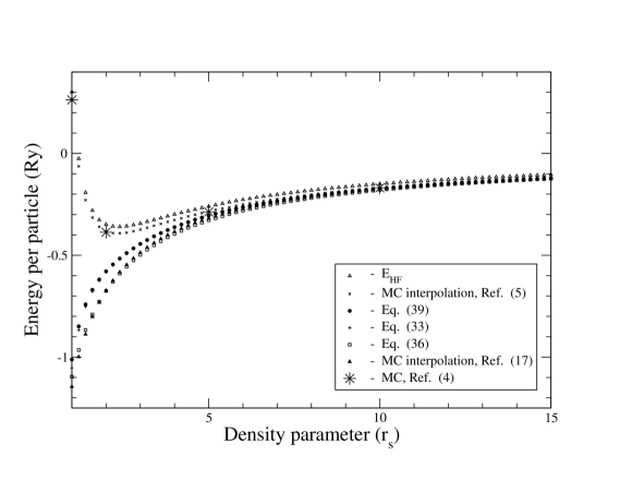
Figure 1: Ground-state energies per particle vs density parameter $r_{s}$ for range $1.0\leq r_{s}\leq 15.0$ from top to bottom: for fermions ($\nu=1$) HF approximation (Eq.  (46) and Ref.  rajagopal , open triangles), MC interpolation data (from Ref.  tanatar , crosses), and present results from Eq.  (44) (closed circles) and Eq.  (36) (plus signs), and for bosons ($\nu=0$) present results from Eq.  (41) (open squares) and MC data from Ref.  DePalo (closed triangles). MC data of Ref.  attac for some particular values of $r_{s}$ are indicated by star symbols.

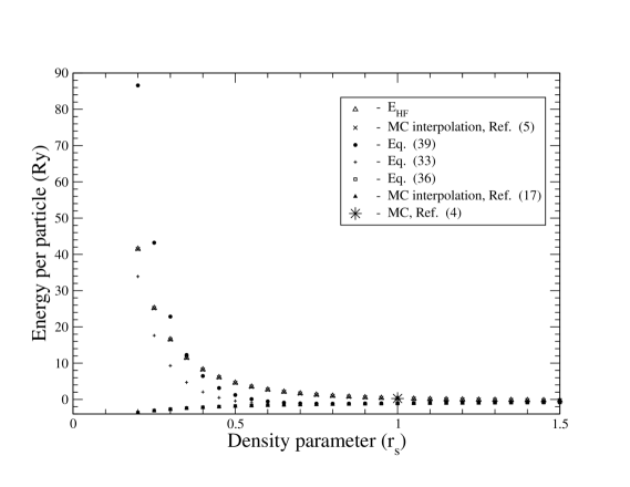
Figure 2: The same as in Fig. 1, however, for range $0.2\leq r_{s}\leq 1.5$.

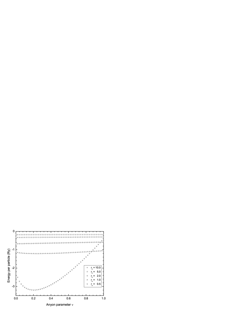
Figure 3: Ground-state energies per particle vs anyon parameter $\nu$ for various fixed values of $r_{s}$.

VI Conclusions

We have derived an approximate analytic formula for the ground-state energy of the Coulomb anyon gas. Starting from our previous results for the noninteracting 2$D$ anyon gas confined in a harmonic potential, we have flattened out the confinement with simultaneous increasing of the particle number to obtain the thermodynamic limit at fixed density. We have generalized this result to describe the interacting 2$D$ Coulomb anyon gas by introducing a function of the anyon parameters $\nu$ and $r_{s}$, that takes into account the Coulomb interaction and fractional statistics. We have determined this function by fitting to the analytic expressions for the ground-state energy of the classical electron crystal at very large $r_{s}$, to that of the 2$D$ Coulomb Bose gas at very small $r_{s}$ and to the HF energy (at high density) for spin-polarized 2$D$ electrons. Our analytic formula applies to the full range of parameters $\nu$ and $r_{s}$ and provides a convenient description of the ground-state of 2$D$ Coulomb anyon systems. By comparison with HF and MC results from the literature we find significant deviations for intermediate densities, which indicate shortcomings of these approaches.

VII Acknowledgments

B. A. and M. M. acknowledge support received from the Volkswagen Foundation and the hospitality at the University of Regensburg. We thank G. Ortiz for the idea of harmonic potential regularization to obtain the thermodynamic limit and M. Seidl for stimulating discussions.

References

- (1) Ch. Kittel, Quantum Theory of Solids (Wiley, New York, 1963).
- (2) G. F. Giuliani and G. Vignale, Quantum Theory of the Electron Liquid (Cambridge University Press, New York, 2005).
- (3) R. M. Dreizler and E. K. Gross, Density Functional Theory: An Approach to the Quantum Many-Body Problem (Springer, Berlin, 1990).
- (4) C. Attaccalite, S. Moroni, P. Gori-Giorgi, and G. B. Bachelet, Phys. Rev. Lett. 88, 256601 (2002); 91, 109902(E) (2003).
- (5) B. Tanatar and D. M. Ceperley, Phys. Rev. B 39, 5005 (1989).
- (6) M. Seidl, Phys. Rev. B 70, 073101 (2004).
- (7) A. Wensauer and U. Rössler, Phys. Rev. B 69, 155301 (2004).
- (8) J. M. Leinaas and J. Myrheim, Nuovo Cimento Soc. Ital. Fis., B 37, 1 (1977).
- (9) F. Wilczek, Phys. Rev. Lett. 48, 1144 (1982).
- (10) F. Wilczek, Fractional Statistics and Anyon Superconductivity (World Scientific, Singapore, 1990).
- (11) S. Forte, Rev. Mod. Phys. 64, 193 (1992); R. Iengo and K. Lechner, Phys. Rep. 213, 179 (1992); Quantum Hall Effect, edited by M. Stone (World Scientific, Singapore, 1992).
- (12) A. Lerda, Anyons (Springer-Verlag, Berlin, 1992).
- (13) A. Khare, Fractional Statistics and Quantum Theory, 2nd ed. (World Scientific, Singapore, 2005).
- (14) A.Yu. Kitaev, Ann. Phys. (N.Y.) 303, 2 (2003).
- (15) Y. Kwon, D. M. Ceperley, and R. M. Martin, Phys. Rev. B 48, 12037 (1993).
- (16) L. Bonsal and A. A. Maradudin, Phys. Rev. B 15, 1959 (1977).
- (17) S. De Palo, S. Conti, and S. Moroni, Phys. Rev. B 69, 035109 (2004).
- (18) L. L. Foldy, Phys. Rev. 124, 649 (1961); see also in N. M. March, W. H. Young, and S. Sampanthar The Many Body Problems in Quantum Mechanics (Cambridge University Press, Cambridge, England, 1967).
- (19) B. Abdullaev, G. Ortiz, U. Rössler, M. Musakhanov, and A. Nakamura, Phys. Rev. B 68, 165105 (2003).
- (20) R. Chitra and D. Sen, Phys. Rev. B 46, 10923 (1992).
- (21) Y. -S. Wu, Phys. Rev. Lett. 53, 111 (1984); 53, 1028(E) (1984).
- (22) R. B. Laughlin, Phys. Rev. Lett. 60, 2677 (1988).
- (23) D. Sen and R. Chitra, Phys. Rev. B 45, 881 (1992).
- (24) X. G. Wen and A. Zee, Phys. Rev. B 41, 240 (1990).
- (25) H. Mori, Phys. Rev. B 42, 184 (1990).
- (26) R. B. Laughlin in The Quantum Hall Effect, edited by R. E. Prange and S. M. Girvin (Springer-Verlag, Berlin, 1987).
- (27) N. N. Bogoliubov, J. Phys. (Moscow) 11, 23 (1947).
- (28) V. Apaja, J. Halinen, V. Halonen, E. Krotscheck, and M. Saarela, Phys. Rev. B 55, 12925 (1997).
- (29) F. Stern, Phys. Rev. Lett. 18, 546 (1967).
- (30) D. S. Fisher, B. I. Halperin, and R. Morf, Phys. Rev. B 20, 4692 (1979).
- (31) A. K. Rajagopal and J. C. Kimball, Phys. Rev. B 15, 2819 (1977).