Generalized Statistics Framework for Rate Distortion Theory with Bregman Divergences

Abstract

A variational principle for the rate distortion (RD) theory with Bregman divergences is formulated within the ambit of the generalized (nonextensive) statistics of Tsallis. The Tsallis-Bregman RD lower bound is established. Alternate minimization schemes for the generalized Bregman RD (GBRD) theory are derived. A computational strategy to implement the GBRD model is presented. The efficacy of the GBRD model is exemplified with the aid of numerical simulations.

I Introduction

The generalized (nonextensive) statistics of Tsallis [1,2] has recently been the focus of much attention in statistical physics, and allied disciplines . Nonextensive statistics generalizes the extensive Boltzmann-Gibbs statistics, and has found much utility in complex systems possessing long range correlations, fluctuations, ergodicity, chirality and fractal behavior. By definition, the Tsallis entropy is defined in terms of discrete variables as

$$S_{q}\left(x\right)=-\frac{{1-\sum\limits_{x}{p^{q}\left(x\right)}}}{{1-q}},where,\sum\limits_{x}{p\left(x\right)}=1.$$ (1)

The constant $q$ is referred to as the nonextensivity parameter. Given two independent variables $x$ and $y$, one of the fundamental consequences of nonextensivity is demonstrated by the pseudo-additivity relation

$$S_{q}\left({xy}\right)=S_{q}\left(x\right)+S_{q}\left(y\right)+\left({1-q}\right)S_{q}\left(x\right)S_{q}\left(y\right).$$ (2)

Here, (1) and (2) imply that extensive statistics is recovered as $q\to 1$. Taking the limit $q\to 1$ in (1) and evoking l’Hospital’s rule, $S_{q}\left(x\right)\to S\left(x\right)$, the Shannon entropy. The jointly convex generalized Kullback-Leibler divergence (K-Ld) is of the form [3]

$$I_{q}\left({p\left(x\right)\left\|{r\left(x\right)}\right.}\right)=\sum\limits_{x}{p\left(x\right)}\frac{{\left({\frac{{p\left(x\right)}}{{r\left(x\right)}}}\right)^{q-1}-1}}{{q-1}}.\$$ (3)

In the limit $q\to 1$, the extensive K-Ld is readily recovered. Akin to the Tsallis entropy, the generalized K-Ld obeys the pseudo-additivity relation [3].

Defining the q-deformed logarithm and the q-deformed exponential as [4]

$$ln_{q}\left(x\right)=\frac{{x^{1-q}-1}}{{1-q}},$$ (4)

and

$$e_{q}^{x}=\left\{\begin{array}[]{l}\left[{1+\left({1-q}\right)x}\right]^{{}^{{\raise 1.50693pt\hbox{$1$}\!\mathord{\left/{\vphantom{1{\left({1-q}\right)}}}\right.\kern-1.2pt}\!\lower 1.50693pt\hbox{${\left({1-q}\right)}$}}}};1+\left({1-q}\right)x\geq 0\\ 0;otherwise,\\ \end{array}\right.$$ (5)

respectively. The Tsallis entropy (1), and, the generalized K-Ld (3) may be written as

$$S_{q}\left({p\left(x\right)}\right)=-\sum\limits_{x}{p\left(x\right)}^{q}\ln_{q}p\left(x\right),$$ (6)

and,

$$I_{q}\left({p\left(x\right)\left\|{r(x)}\right.}\right)=-\sum\limits_{x}{p\left(x\right)}\ln_{q}\frac{{r(x)}}{{p(x)}},$$ (7)

respectively. Employing the relation [4]

$$\ln_{q}\left({\frac{x}{y}}\right)=y^{q-1}\left({\ln_{q}x-\ln_{q}y}\right),$$ (8)

the generalized K-Ld (7) may be expressed as the generalized mutual information

$$\begin{array}[]{l}I_{q}\left({X;\tilde{X}}\right)=-\sum\limits_{x,\tilde{x}}{p\left({x,\tilde{x}}\right)\ln_{q}}\left({\frac{{p\left({\tilde{x}}\right)}}{{p\left({\left.{\tilde{x}}\right|x}\right)}}}\right)\\ =\sum\limits_{\tilde{x}}{\frac{1}{{p^{q-1}\left({\tilde{x}}\right)}}}S_{q}\left(X\right)-\underbrace{\sum\limits_{\tilde{x}}{p\left({\tilde{x}}\right)}S_{q}\left({\left.X\right|\tilde{X}=\tilde{x}}\right)}_{\left\langle{S_{q}\left({\left.X\right|\tilde{X}=\tilde{x}}\right)}\right\rangle_{p\left({\tilde{x}}\right)}}.\\ \end{array}$$ (9)

Here, $\left\langle\bullet\right\rangle$ denotes the expectation value. The seminal paper on source coding within the framework of nonextensive statistics by Landsberg and Vedral [5], has provided the impetus for a number of investigations into the use of nonextensive information theory within the context of coding problems. The works of Yamano [6,7] represent a sample of some of the prominent efforts in this regard. The source coding theorem in a nonextensive setting has been derived by Yamano [8].

A statistical physics model for the variational problem encountered in rate distortion (RD) theory [9, 10] and the information bottleneck method [11], derived within a generalized statistics framework, has been recently established [12]. A nonextensive Blahut-Arimorto (BA) alternate minimization scheme [13] has been derived. The noteworthy result of the study in [12] is that the nonextensive RD curves possesses a lower threshold for the minimum compression information in the distortion-compression plane, as compared to equivalent RD curves derived on the basis of the Boltzmann-Gibbs-Shannon framework. As was the case in [12], this paper employs values of $q$ in the range $0<q<1$. This paper utilizes the statistical physics theory presented in [12] to formulate a generalized Bregman RD (GBRD) model. The GBRD model extends previous works by Rose [14] and Banerjee et. al. [15, 16] to achieve a principled and practical strategy to evaluate RD functions.

II Rationale for the GBRD model

II-A Background information

The RD problem in terms of discrete random variables is stated as follows: given a discrete random variable $X\in\Xi$ called the source or the codebook, and, another discrete random variable $\tilde{X}\in\tilde{\Xi}$ which is a compressed representation of $X$ (also referred to as the quantized codebook and/or the reproduction alphabet), the information rate distortion function that is to be obtained is the minimization of the mutual information $I_{q\geq 1}(X,\tilde{X})$ over all conditional probabilities $p\left({\tilde{x}\left|x\right.}\right)$.

The crux of the RD problem is the numerical determination of the RD function using the BA scheme. The actual implementation of the BA scheme is sometimes impractical owing to a lack of knowledge of the optimal support of the quantized codebook $\tilde{X}$. Exact analytical solutions exist only for a few cases consisting of a combination well behaved sources and distortion measures. An initial attempt to achieve a practical and tractable solution to the RD problem was performed by Rose [14], for the case of Euclidean square distortion functions. Therein, it was demonstrated that for sources whose support is a bounded set, the RD function either equals the Shannon lower bound, or, the optimal support for the quantized codebook is finite thus permitting the use of a numerical procedure called the mapping method. The pioneering work of Rose was generalized by Banerjee et. al [15, 16] to include a wider class of distortion functions using Bregman divergences. One of the significant features in these works involved the formulation of a Shannon-Bregman lower bound.

Motivated by the recent results [12], this paper provides two means to solve the GBRD problem for sources with bounded support. First, the analytical solution may be obtained from a Tsallis-Bregman lower bound (Section IV). Next, for a finite reproduction alphabet, the RD function may be numerically obtained by a computational methodology derived from generalized statistics (Section III).

II-B Bregman Divergences

Definition 1 (Bregman divergences): Let $\phi$ be a real valued strictly convex function defined on the convex set $S\subseteq\Re$, the domain of $\phi$ such that $\phi$ is differentiable on $int(S)$, the interior of $S$. The Bregman divergence $B_{\phi}:S\times{\mathop{\rm int}}\left(S\right)\mapsto\Re^{+}$ is defined as $B_{\phi}\left({z_{1},z_{2}}\right)=\phi\left({z_{1}}\right)-\phi\left({z_{2}}\right)-\left({z_{1}-z_{2},\nabla\phi\left({z_{2}}\right)}\right)$, where $B_{\phi}\left({z_{1},z_{2}}\right)=\phi\left({z_{1}}\right)-\phi\left({z_{2}}\right)-\left({z_{1}-z_{2},\nabla\phi\left({z_{2}}\right)}\right)$ is the gradient of $\phi$ evaluated at $z_{2}$.

A number of Bregman divergences have been tabulated in [15]. The generalized K-Ld in (3), also referred to as the Csiszár generalized K-Ld is not a Bregman divergence. Since the seminal work by Naudts [17], Bregman divergences have been the object of much research in nonextensive statistics. Defining $\phi(p)=-p\ln_{q}\left({{\raise 3.01385pt\hbox{$1$}\!\mathord{\left/{\vphantom{1p}}\right.\kern-1.2pt}\!\lower 3.01385pt\hbox{$p$}}}\right)$, the Bregman generalized K-Ld is defined as

$$\begin{array}[]{l}d_{\phi}\left({\textbf{p},\textbf{r}}\right)=\sum\limits_{i=1}^{d}{\frac{{p_{i}}}{{\left({q-1}\right)}}}\left({p_{i}^{q-1}-r_{i}^{q-1}}\right)-\sum\limits_{i=1}^{d}{\left({p_{i}-r_{i}}\right)}r_{i}^{q-1}\\ =I_{q,B}\left({\left.\textbf{p}\right\|\textbf{r}}\right)\end{array}$$ (10)

Setting $q-1\to\kappa$, (10) is consistent with Eq. (35) in [17].

III the GBRD model

This Section provides a strategy to jointly obtain the optimal support $\tilde{\mathcal{X}}_{s}$ of the quantized codebook with cardinality $\left|{\tilde{\mathcal{X}}_{s}}\right|=k$ , and, the conditional probability $p(\tilde{x}|x)$ that characterizes the RD problem. This is accomplished by a joint optimization of

$$\mathop{\min}\limits_{\tilde{\mathcal{X}}_{s},p\left({\left.{\tilde{x}}\right|x}\right)}L_{GBRD}^{q}=\mathop{\min}\limits_{\scriptstyle\tilde{\mathcal{X}}_{s},p\left({\left.{\tilde{x}}\right|x}\right)\hfill\atop\scriptstyle\left|{\tilde{\mathcal{X}}_{s}}\right|=k\hfill}\left\{{I_{q}\left({X;\tilde{X}}\right)+\beta\left\langle{d_{\phi}\left({x,\tilde{x}}\right)}\right\rangle_{p\left({x,\tilde{x}}\right)}}\right\}.$$ (11)

The optimal Lagrange multiplier $\beta$, hereafter referred to as the inverse temperature, depends upon the optimal tolerance level of the expectation of $D=<d_{\phi}(x,\tilde{x})>_{p(x,\tilde{x})}=\sum\limits_{x,\tilde{x}}{p\left({x,\tilde{x}}\right)}d_{\phi}\left({x,\tilde{x}}\right)$.

III-A Constraint terms

Generalized statistics has utilized a number of constraints to define expectations. The original Tsallis (OT) constraints of the form $\left\langle A\right\rangle=\sum\limits_{i}{p_{i}}A_{i}$ [1], were convenient owing to their similarity to the maximum entropy constraints. These were abandoned because of difficulties encountered in obtaining an acceptable form for the partition function, with the exception of a few specialized cases.

The OT constraints were subsequently replaced by the Curado-Tsallis (C-T) constraints $\left\langle A\right\rangle_{q}^{C-T}=\sum\limits_{i}{p_{i}^{q}}A_{i}$. The C-T constraints were later replaced by the normalized Tsallis-Mendes-Plastino (T-M-P) constraints $\left\langle A\right\rangle^{T-M-P}=\sum\limits_{i}{\frac{{p_{i}^{q}}}{{\sum\limits_{i}{p_{i}^{q}}}}A_{i}}$. The dependence of the expectation value on the normalization pdf ${\sum\limits_{i}{p_{i}^{q}}}$, renders the T-M-P constraints to be self-referential. This paper, like [12], utilizes a recent methodology [18] to “rescue” the OT constraints, and, has linked the OT, C-T, and, T-M-P constraints.

III-B The nonextensive variational principle

Keeping $\tilde{\mathcal{X}}_{s}$ fixed, taking the variational derivative of (11) with respect to $p(\tilde{x}|x)$ while enforcing $\sum\limits_{\tilde{x}}{p\left({\left.{\tilde{x}}\right|x}\right)}=1$ with the normalization Lagrange multiplier $\lambda(x)$, yields

$$\begin{array}[]{l}p\left({\tilde{x}\left|x\right.}\right)=p\left({\tilde{x}}\right)\left[{\frac{(1-q)}{{q}}\left\{{\tilde{\lambda}\left(x\right)+\beta d_{\phi}\left({x,\tilde{x}}\right)}\right\}}\right]^{1/\left({q-1}\right)},\\ \\ \tilde{\lambda}\left(x\right)=\frac{{\lambda\left(x\right)}}{{p\left(x\right)}}-p\left(x\right)^{\left({1-q}\right)}.\\ \end{array}$$ (12)

Multiplying the terms in the square brackets in (12) by the conditional probability $p\left({\left.{\tilde{x}}\right|x}\right)$, and summing over $\tilde{x}$ yields

$$\begin{array}[]{l}\frac{q}{{q-1}}\sum\limits_{\tilde{x}}{p\left({\tilde{x}}\right)\left({\frac{{p\left({\left.{\tilde{x}}\right|x}\right)}}{{p\left({\tilde{x}}\right)}}}\right)^{q}}+\underbrace{\beta\sum\limits_{\tilde{x}}{d_{\phi}\left({x,\tilde{x}}\right)p\left({\left.{\tilde{x}}\right|x}\right)}}_{\beta\left\langle{d_{\phi}\left({x,\tilde{x}}\right)}\right\rangle_{p\left({\left.{\tilde{x}}\right|X=x}\right)}}+\\ +\tilde{\lambda}\left(x\right)\sum\limits_{\tilde{x}}{p\left({\left.{\tilde{x}}\right|x}\right)=0}.\\ \end{array}$$ (13)

Evoking $\sum\limits_{\tilde{x}}{p\left({\left.{\tilde{x}}\right|X=x}\right)}=1$, yields

$$\tilde{\lambda}\left(x\right)=\frac{q}{{\left({1-q}\right)}}\aleph_{q}\left(x\right)-\beta\left\langle{d_{\phi}\left({x,\tilde{x}}\right)}\right\rangle_{p\left({\left.{\tilde{x}}\right|X=x}\right)}.$$ (14)

Here, $\aleph_{q}\left(x\right)=\sum\limits_{\tilde{x}}{p\left({\tilde{x}}\right)\left({\frac{{p\left({\left.{\tilde{x}}\right|x}\right)}}{{p\left({\tilde{x}}\right)}}}\right)^{q}}$. The conditional pdf $p\left({\left.{\tilde{x}}\right|x}\right)$ acquires the form

$$\begin{array}[]{l}p\left({\left.{\tilde{x}}\right|x}\right)=\frac{{p\left({\tilde{x}}\right)\left\{{1-\left({q-1}\right)\beta^{*}d_{\phi}\left({x,\tilde{x}}\right)}\right\}^{1/\left({q-1}\right)}}}{{\Im_{RD}^{{}^{1/\left({1-q}\right)}}}},\\ \Im_{RD}=q\aleph_{q}\left(x\right)+\left({q-1}\right)\beta\left\langle{d_{\phi}\left({x,\tilde{x}}\right)}\right\rangle_{p\left({\left.{\tilde{x}}\right|X=x}\right)},\\ \beta^{*}=\frac{\beta}{\Im_{RD}},\end{array}$$ (15)

where $\beta^{*}$ is the effective inverse temperature. Transforming $q\to 2-q^{*}$ in the numerator and evoking (5), (15) is expressed in the form of a q-deformed exponential

$$p\left({\tilde{x}\left|x\right.}\right)=\frac{{p\left({\tilde{x}}\right)\exp_{q^{*}}(-\beta^{*}d_{\phi}\left({x,\tilde{x}})\right)}}{\tilde{Z}(x,\beta^{*})}.$$ (16)

The partition function evaluated at each instance of the source distribution is

$$\tilde{Z}\left({x,\beta^{*}}\right)=\Im_{RD}^{\frac{1}{{\left({1-q}\right)}}}=\sum\limits_{\tilde{x}}{p\left({\tilde{x}}\right)\exp_{q}}\left[{-\beta^{*}d_{\phi}\left({x,\tilde{x}}\right)}\right]$$ (17)

The term $\left\{{1-\left({1-q^{*}}\right)\beta^{*}d\left({x,\tilde{x}}\right)}\right\}$ in the numerator of (16) is a manifestation of the Tsallis cut-off condition [18]. This implies that solutions of (16) are valid when $\beta^{*}d\left({x,\tilde{x}}\right)<{\raise 3.01385pt\hbox{$1$}\!\mathord{\left/{\vphantom{1{\left({1-q^{*}}\right)}}}\right.\kern-1.2pt}\!\lower 3.01385pt\hbox{${\left({1-q^{*}}\right)}$}}$. The effective nonextensive RD Helmholtz free energy is

$$F_{RD}^{q}\left({\beta^{*}}\right)=\frac{{-1}}{{\beta^{*}}}\left\langle{\ln_{q}\tilde{Z}\left({x,\beta^{*}}\right)}\right\rangle_{p\left(x\right)}=\frac{1}{{\beta^{*}}}\left\langle{\frac{{\Im_{RD}-1}}{{q-1}}}\right\rangle_{p\left(x\right).}$$ (18)

Solution of (16) may be viewed from two distinct perspectives, i.e. the canonical perspective and the parametric perspective. Owing to the self-referential nature of the effective inverse temperature $\beta^{*}$, the analysis and solution of (16) within the context of the canonical perspective is a formidable undertaking. For practical applications, the parametric perspective is utilized by evaluating the conditional pdf $p\left({\left.{\tilde{x}}\right|x}\right)$, employing the nonextensive BA algorithm, for a-priori specified $\beta^{*}\in\left[{0,\infty}\right]$. Note that within the context of the parametric perspective, the self-referential nature of $\beta^{*}$ vanishes. The inverse temperature $\beta$ and the effective inverse temperature $\beta^{*}$ relate as

$$\beta=\frac{{q\aleph_{q}\left(x\right)\beta^{*}}}{{\left[1-{\beta^{*}\left({q-1}\right)\left\langle{d_{\phi}\left({x,\tilde{x}}\right)}\right\rangle_{p\left({\left.{\tilde{x}}\right|X=x}\right)}}\right]}}.$$ (19)

III-C Support estimation step

The procedure in Section III.B. is carried out for a given $\beta$, corresponding to a single point on the RD curve. Reproduction alphabets with optimal support are obtained by keeping $p(\tilde{x}|x)$ fixed, and solving

$$\mathop{\min}\limits_{\tilde{\mathcal{X}}_{s}}L_{GBRD}^{q}=\mathop{\min}\limits_{\scriptstyle\tilde{\mathcal{X}}_{s}}\left\{{I_{q}\left({X;\tilde{X}}\right)+\beta\left\langle{d_{\phi}\left({x,\tilde{x}}\right)}\right\rangle_{p\left({x,\tilde{x}}\right)}}\right\}.$$ (20)

The solution to (20) is the optimal estimate/predictor [15, 16]

$$\tilde{x}^{*}=\left\langle x\right\rangle_{p\left({\left.x\right|\tilde{X}=\tilde{x}}\right)}=\sum\limits_{x}{p\left({\left.x\right|\tilde{X}=\tilde{x}}\right)x}.$$ (21)

Algorithm 1 depicts the pseudo-code for the greedy joint non-convex optimization procedure that constitutes the solution to the GBRD model.

IV the Tsallis-Bregman lower bound

Theorem 1 For OT constraints, the nonextensive RD function with source $X\sim p(x)$ and a Bregman divergence $d_{\phi}$ is always lower bounded by the Tsallis-Bregman lower bound defined by

$$\begin{array}[]{l}R_{qL}\left(D\right)=\sum\limits_{\tilde{x}}{\frac{1}{{p^{q-1}\left({\tilde{x}}\right)}}}S_{q}\left(X\right)+\\ +\mathop{\sup}\limits_{\beta\geq 0}\left\{{-\beta D+\left\langle{\ln_{q^{*}}\gamma_{L,\beta^{*}}\left(x\right)}\right\rangle_{p\left(x\right)}}\right\},\end{array}$$ (22)

where $\gamma_{L\beta^{*}}$ is a unique function satisfying

$$\int_{dom(\phi)}{p\left(t\right)\gamma_{L,\beta^{*}}\left(t\right)\exp_{q^{*}}\left({-\beta^{*}d_{\phi}\left({t,\mu}\right)}\right)dt}=1;\forall\mu\in dom\left(\phi\right).$$ (23)

To highlight the critical dependence of the Tsallis-Bregman lower bound upon the type of constraint employed to solve the GBRD variational problem in Section III B, and enunciate certain aspects of q-deformed algebra and calculus, a slightly weaker bound (see Appendix C, [16]) is stated and proved.

Theorem 2 The generalized RD function is defined by

$$R_{q}\left(D\right)=\mathop{\sup}\limits_{\beta\geq 0,\gamma^{*}\in\Lambda_{\beta^{*}}}\left\{{-\beta D+\int_{x}{p\left(x\right)\ln_{q^{*}}\gamma^{*}\left(x\right)dx}}\right\},$$ (24)

where ${\Lambda_{\beta^{*}}}$ is the set of all admissible partition functions. Further, for each ${\beta\geq 0}$, a necessary and sufficient condition for $\gamma^{*}\left(x\right)$ to attain the supremum in (24)is a probability density $p(\tilde{x})$ related to $\gamma^{*}(x)$ as

$$\gamma^{*}\left(x\right)=\left({\int_{\tilde{x}}{p\left({\tilde{x}}\right)}\exp_{q}\left({-\beta^{*}d_{\phi}\left({x,\tilde{x}}\right)}\right)d\tilde{x}}\right)^{-1}.$$ (25)

Proof

$$\begin{array}[]{l}L_{GBRD}^{q}\left[p({\left.{\tilde{x}}\right|x}\right)]=\\ -\int_{x,\tilde{x}}{p\left(x\right)}p\left({\left.{\tilde{x}}\right|x}\right)\ln_{q}\left({\frac{{p\left({\tilde{x}}\right)}}{{p\left({\left.{\tilde{x}}\right|x}\right)}}}\right)dxd\tilde{x}+\\ +\beta\int_{x,\tilde{x}}{p\left(x\right)}p\left({\left.{\tilde{x}}\right|x}\right)d_{\phi}\left({x,\tilde{x}}\right)dxd\tilde{x}\\ \mathop{=}\limits^{\left(a\right)}\int_{x,\tilde{x}}{p\left(x\right)}p\left({\left.{\tilde{x}}\right|x}\right)\ln_{q^{*}}\left({\frac{{p\left({\left.{\tilde{x}}\right|x}\right)}}{{p\left({\tilde{x}}\right)}}}\right)dxd\tilde{x}+\\ +\beta\int_{x,\tilde{x}}{p\left(x\right)}p\left({\left.{\tilde{x}}\right|x}\right)d_{\phi}\left({x,\tilde{x}}\right)dxd\tilde{x}\\ \mathop{=}\limits^{\left(b\right)}\int_{x,\tilde{x}}{p\left(x\right)}p\left({\left.{\tilde{x}}\right|x}\right)\ln_{q^{*}}\left({\frac{{\exp_{q^{*}}\left({-\beta^{*}d_{\phi}\left({x,\tilde{x}}\right)}\right)}}{{\tilde{Z}\left({x,\beta^{*}}\right)}}}\right)dxd\tilde{x}+\\ +\beta\int_{x,\tilde{x}}{p\left(x\right)}p\left({\left.{\tilde{x}}\right|x}\right)d_{\phi}\left({x,\tilde{x}}\right)dxd\tilde{x}\\ \mathop{=}\limits^{\left(c\right)}-\int_{x,\tilde{x}}{p\left(x\right)p\left({\left.{\tilde{x}}\right|x}\right)}\tilde{Z}^{\left({q-1}\right)}\left({x,\beta^{*}}\right)\left({\beta^{*}d_{\phi}\left({x,\tilde{x}}\right)+}\right.\\ \left.{\ln_{q^{*}}\tilde{Z}\left({x,\beta^{*}}\right)}\right)dxd\tilde{x}+\beta\int_{x,\tilde{x}}{p\left(x\right)p\left({\left.{\tilde{x}}\right|x}\right)}d_{\phi}\left({x,\tilde{x}}\right)dxd\tilde{x}\\ \mathop{=}\limits^{\left(d\right)}-\int_{x,\tilde{x}}{p\left(x\right)p\left({\left.{\tilde{x}}\right|x}\right)}\ln_{q}\tilde{Z}\left({x,\beta^{*}}\right)dxd\tilde{x}\\ =-\int_{x}{p\left(x\right)}\ln_{q}\tilde{Z}\left(x,\beta^{*}\right)dx\\ \mathop{=}\limits^{\left(e\right)}-\int_{x}{p\left(x\right)}\ln_{q}\left({\int_{\tilde{x}}{p\left({\tilde{x}}\right)\exp_{q^{*}}\left({-\beta^{*}d_{\phi}\left({x,\tilde{x}}\right)}\right)d\tilde{x}}}\right)dx\\ =L_{GBRD}^{q}\left[p(\tilde{x}\right)].\end{array}$$ (26)

Here, $(a)$ follows from $\ln_{q}\left(x\right)=-\ln_{q^{*}}\left({{\raise 3.01385pt\hbox{$1$}\!\mathord{\left/{\vphantom{1x}}\right.\kern-1.2pt}\!\lower 3.01385pt\hbox{$x$}}}\right);q^{*}=2-q$, $(b)$ follows from (16) where the partition function in the continuum is $\tilde{Z}\left({x,\beta^{*}}\right)=\int_{\tilde{x}}{p\left({\tilde{x}}\right)}\exp_{q}\left({-\beta^{*}d_{\phi}\left({x,\tilde{x}}\right)}\right)d\tilde{x}$, $(c)$ follows from (8), $(d)$ follows from (15), and, $(e)$ follows from (17). Analogous to the mapping method of [14], a mapping from the unit interval to the reproduction alphabet is sought such that the Lebesgue measure over the unit interval results in an optimal $p(\tilde{x})$ over the reproduction alphabet. Thus, for each instance of a probability measure corresponding to $p\left({\tilde{x}}\right)$ on $\tilde{\mathcal{X}}$ there exists a unique map $\tilde{x}:\left[{0,1}\right]\mapsto\tilde{\mathcal{X}}$ that maps the Lebesgue measure ($\mu$) to $p\left({\tilde{x}}\right)$ such that for any function $f$ defined over $\tilde{x}$, $\int_{\tilde{x}}{f\left({\tilde{x}}\right)p\left({\tilde{x}}\right)}d\tilde{x}=\int_{u\in\left[{0,1}\right]}{f\left({\tilde{x}\left(u\right)}\right)}d\mu\left(u\right)$. Thus, (26) yields

$$\begin{array}[]{l}L_{GBRD}^{q}\left[{\tilde{x}}\right]=\\ =-\int_{x}{p\left(x\right)}\ln_{q}\left({\int_{\tilde{x}}{p\left({\tilde{x}}\right)\exp_{q^{*}}\left({-\beta^{*}d_{\phi}\left({x,\tilde{x}}\right)}\right)d\tilde{x}}}\right)dx,\\ =-\int_{x}{p\left(x\right)}\ln_{q}\left({\int_{u\in\left[{0,1}\right]}{\exp_{q^{*}}\left({-\beta^{*}d_{\phi}\left({x,\tilde{x}\left(u\right)}\right)}\right)d\mu\left(u\right)}}\right)dx.\\ \end{array}$$ (27)

To obtain the optimality condition, the q-deformed terms characteristic to generalized statistics are to be operated on by the dual Jackson derivative instead of the usual Newtonian derivative [4]. To obtain expressions analogous to the case of Newton-Leibniz calculus, the dual Jackson derivative defined as

$$\begin{array}[]{l}D^{\left(q\right)}f\left(x\right)=\frac{1}{{1+(1-q)f\left(x\right)}}\frac{{df}}{{dx}};1+(1-q)f\left(x\right)\neq 0\\ \Rightarrow D^{\left(q\right)}\ln_{q}\tilde{Z}\left({x,\beta^{*}}\right)=\frac{1}{{\tilde{Z}\left({x,\beta^{*}}\right)}}\frac{{d\tilde{Z}\left({x,\beta^{*}}\right)}}{{dx}}\end{array}$$ (28)

is employed to enforce the optimality condition. The optimality condition for (27) becomes

$$D^{\left(q\right)}L_{GBRD}^{q}=-\int_{x}{\frac{{p\left(x\right)\frac{d}{{d\tilde{x}}}\left({\exp_{q^{*}}\left({-\beta^{*}d_{\phi}\left({x,\tilde{x}\left(u\right)}\right)}\right)}\right)dx}}{{\int_{u\in\left[{0,1}\right]}{\exp_{q^{*}}\left({-\beta^{*}d_{\phi}\left({x,\tilde{x}\left(u\right)}\right)}\right)ud\mu}}}}.$$ (29)

Evoking Borel isomorphism, and, assuming that the optimal support $\tilde{\mathcal{X}}_{s}$ contains a non-empty open ball $B_{\epsilon}$, $\epsilon>0$ implies that

$$\begin{array}[]{l}D^{\left(q\right)}L_{GBRD}^{\left(q\right)}=\int_{x}{\frac{{p\left(x\right)\exp_{q^{*}}\left({-\beta^{*}d\left({x,\tilde{x}}\right)}\right)dx}}{{N\left({x,\beta^{*}}\right)}}}=k_{o}\forall\tilde{x}\in B_{\epsilon}\subset\tilde{\mathcal{X}}_{s},\\ \Rightarrow\int_{\tilde{x}\in B_{\in}}{\int_{x}{\frac{{p\left(x\right)p\left({\tilde{x}}\right)\exp_{q^{*}}\left({-\beta^{*}d\left({x,\tilde{x}}\right)}\right)dxd\tilde{x}}}{{N\left({x,\beta^{*}}\right)}}}}=k_{o}\int_{\tilde{x}\in B_{\in}}{p\left({\tilde{x}}\right)d\tilde{x}},\\ \Rightarrow\int_{\tilde{x}\in B_{\in}}{\int_{x}{p\left(x\right)p\left({\left.{\tilde{x}}\right|x}\right)dxd\tilde{x}=}}k_{o}\int_{\tilde{x}\in B_{\in}}{p\left({\tilde{x}}\right)d\tilde{x}}\Rightarrow 1=k_{o},\\ \end{array}$$ (30)

holds true for all $\tilde{x}\in B_{\epsilon}$. Defining $\gamma_{\beta^{*}}^{*}\left(x\right)=\left({\int_{\tilde{x}}{p\left({\tilde{x}}\right)}\exp_{q}\left({-\beta^{*}d_{\phi}\left({x,\tilde{x}}\right)}\right)d\tilde{x}}\right)^{-1}$, (30) yields

$$\int_{x}{p\left(x\right)\gamma_{\beta^{*}}^{*}\left(x\right)\exp_{q^{*}}\left({-\beta^{*}d\left({x,\tilde{x}}\right)}\right)dx}=1;\forall\tilde{x}\in B_{\in}.$$ (31)

Using the relation $-\ln_{q}\left(x\right)=\ln_{q^{*}}\left({{\raise 3.01385pt\hbox{$1$}\!\mathord{\left/{\vphantom{1x}}\right.\kern-1.2pt}\!\lower 3.01385pt\hbox{$x$}}}\right)$, (26) becomes

$$L_{GBRD}^{q}\left[{p\left({\tilde{x}}\right)}\right]=\int_{x}{p\left(x\right)\ln_{q^{*}}\gamma_{\beta^{*}}^{*}\left(x\right)}dx.$$ (32)

Thus, $\gamma_{\beta^{*}}^{*}(x)$ satisfies (25) and attains the supremum in (24) for a given $\beta$ and corresponding $\beta^{*}$

$$R_{q}\left({D_{\beta}}\right)=-\beta D_{\beta}+\int_{x}{p\left(x\right)\ln_{q^{*}}\gamma_{\beta^{*}}^{*}\left(x\right)dx},$$ (33)

where $D_{\beta}$ is the distortion value at which the supremum in (24) is attained for a given $\beta$. Thus, the Tsallis-Bregman lower bound is

$$R_{qL}\left({D_{\beta}}\right)=-\beta D_{\beta}+\int_{x}{p\left(x\right)\ln_{q^{*}}\gamma_{\beta^{*}}^{*}\left(x\right)dx}=R_{q}\left({D_{\beta}}\right).$$ (34)

Algorithm 1 GBRD Model

  Input 1. $X\sim p(x)$ over $\left\{{x_{i}}\right\}_{i=1}^{n}\subset dom\left(\phi\right)\subseteq\Re^{m}$.2. Bregman divergence $d_{\phi}$, $|\tilde{\mathcal{X}}_{s}|=k$, effective variational parameter $\beta^{*}\in\left[{0,\infty}\right]$, each $\beta^{*}$ is a single point on the RD curve.

  Output 1.$\tilde{\mathcal{X}}_{s}^{*}=\left\{{\tilde{x}}\right\}_{j=1}^{k},P^{*}=\left\{{\left\{{\left.{\tilde{x}_{j}}\right|x_{i}}\right\}_{j=1}^{k}}\right\}_{i=1}^{n}$ that locally optimizes (11), $(R_{\beta},D_{\beta})$ tradeoff at each $\beta^{*}$ 2.Value of $R_{q}(D)$ where its slope equals $-\beta=\frac{{-q\aleph_{q}\left(x\right)\beta^{*}}}{{\left[1-{\beta^{*}\left({q-1}\right)\left\langle{d_{\phi}\left({x,\tilde{x}}\right)}\right\rangle_{p\left({\left.{\tilde{x}}\right|X=x}\right)}}\right]}}.$

  Method 1.Initialize with some $\left\{{\tilde{x}}\right\}_{j=1}^{k}\subset dom\left(\phi\right)$. 2.Set up outer $\beta^{*}$ loop. repeatBlahut-Arimoto loop (16) for single value of $\beta^{*}$repeat for i=1 to $n$ do for j=1 to $k$ do $p\left({\tilde{x}_{j}\left|x_{i}\right.}\right)\leftarrow\frac{{p\left({\tilde{x}_{j}}\right)\exp_{q^{*}}(-\beta^{*}d_{\phi}\left({x_{i},\tilde{x}_{j}})\right)}}{\tilde{Z}(x_{i},\beta^{*})}$ end for end for for j=1 to $k$ do $p\left({\tilde{x}_{j}}\right)\leftarrow\sum\nolimits_{i=1}^{n}{p\left({\left.{\tilde{x}_{j}}\right|x_{i}}\right)p\left({x_{i}}\right)}$ end for until convergence Support Estimation Step ($\tilde{\mathcal{X}}_{s}$ using (21)) for j=1 to $k$ do $\tilde{x}_{j}\leftarrow\sum\nolimits_{i=1}^{n}{p\left({\left.{x_{i}}\right|\tilde{x}_{j}}\right)}x_{i}$ end for until convergence Calculate $D_{\beta}$ and $R_{\beta}$ for the $\beta^{*}$. advance $\beta^{*}$ $\beta^{*}=\beta^{*}+\delta\beta^{*}$

V Numerical simulations

The efficacy of the GBRD model is computationally investigated by drawing a sample of 1000 two-dimensional data points, from three spherical Gaussian distributions with centers $(2,3.5),(0,0),(0,2)$ (the quantized codebook). The priors and standard deviations are $0.3,0.4,0.3$, and, $0.2,0.5,1.0$, respectively. To test effectiveness of the support estimation step, the quantized codebook is shifted from the true means to positions at the edges of the spherical Gaussian distributions. The computational procedure described in Algorithm 1 is repeatedly solved for each value of $\beta^{*}$, till a reproduction alphabet with optimal support is obtained. This consistently coincides with the true mean, for a negligible error. This effect is particularly pronounced, and rapidly achieved, for regions of low and intermediate values of $\beta^{*}$, thus providing implicit proof of the relation between soft clustering and RD with Bregman divergences [15].

Fig.1 depicts the RD curves for extensive RD with Bregman divergences [15, 16] and the GBRD model, with the constituent discrete points overlaid upon them. A Euclidean square distortion (a Bregman divergence) is employed. Each curve has been generated for values of $\beta\in\left[{.1,2.5}\right]$ (the extensive case), and $\beta^{*}\in\left[{.1,100}\right]$ (the GBRD cases), respectively. Note that for the GBRD cases, the slope of the RD curve is $-\beta$ and not $-\beta^{*}$. Note that all GBRD curves inhabit the non-achievable (no compression) region of the extensive RD model with Bregman divergences. Further, GBRD models possessing a lower nonextensivity parameter $q$ inhabit the non-achievable regions of GBRD models possessing a higher value of $q$. It is observed that the GBRD model undergoes compression and clustering more rapidly than the equivalent extensive RD model with Bregman divergences. A primary cause for such behavior is the rapid increase in $\beta^{*}$ for marginal increases in $\beta$, as depicted in Fig. 2 and obtained from (19).

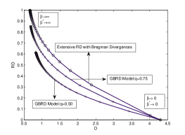
Figure 1: Rate Distortion Curves for GBRD Model and Extensive RD with Bregman Divergences

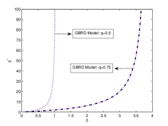
Figure 2: Curves for $\beta$ v/s $\beta^{*}$ for GBRD Model

References

• [1] C. Tsallis. Possible Generalizations of Boltzmann-Gibbs Statistics. J. Stat. Phys., 542, pp 479-487, 1988.
• [2] M. Gell-Mann and C. Tsallis (Eds.). Nonextensive Entropy-Interdisciplinary Applications. Oxford University Press, New York, 2004.
• [3] C. Tsallis. Generalized Entropy-Based Criterion for Consistent Testing. Phys. Rev. E, 58, pp 1442-1445, 1998.
• [4] E. Borges. A Possible Deformed Algebra and Calculus Inspired in Nonextensive Thermostatistics. Physica A, 340, pp. 95-111, 2004. Manuscript available at http://arxiv.org/abs/cond-mat/0304545.
• [5] P.T. Landsberg and V. Vedral. Distributions and Channel Capacities in Generalized Statistical Mechanics. Phys. Lett. A, 247, pp. 211-217, 1998.
• [6] T. Yamano. Information Theory based on Nonadditive Information Content. Phys. Rev. E, 63, pp. 046105-046111, 2001.
• [7] T. Yamano. Generalized Symmetric Mutual Information Applied for the Channel Capacity. Phys. Rev. E., To Appear. Manuscript available at http://arxiv.org/abs/cond-mat/0102322.
• [8] T. Yamano. Source Coding Theorem based on a Nonadditive Information Content. Physica A, 305,1, pp. 190-195, 2002.
• [9] T. Cover and J. Thomas. Elements of Information Theory. John Wiley $\ \&$ Sons, New York, NY, 1991.
• [10] T. Berger. Rate Distortion Theory. Prentice-Hall, Englewood Cliffs, NJ, 1971.
• [11] N. Tishby, F. C. Pereira, W. Bialek. The Information Bottleneck Method . Proceedings of the $37^{th}$ Annual Allerton Conference on Communication, Control and Computing, pp 368-377, 1999.
• [12] R. C. Venkatesan. Generalized Statistics Framework for Rate Distortion Theory. Physica A, To Appear, 2007. Preliminary manuscript available at http://arxiv.org/abs/cond-mat/0611567.
• [13] R. E. Blahut. Computation of Channel Capacity and Rate Distortion Functions. IEEE Trans. on Inform. Theory, IT 18, pp. 460 473, 1972.
• [14] K. Rose. A Mapping Approach to Rate Distortion Computation and Analysis. IEEE Trans. on Inform. Theory, 40,6 pp. 1939 1952, 1994.
• [15] A. Banerjee, S. Merugu, I. Dhillon, and, J. Ghosh. Clustering with Bregman Divergences. Journal of Machine Learning Research (JMLR), 6, pp 1705-1749, 2005.
• [16] A. Banerjee. Scalable Clustering Algorithms Ph.D. dissertation, The University of Texas at Austin, 2005.
• [17] J. Naudts. Continuity of a Class of Entropies and Relative Entropies. Rev. Math. Phys., 16, pp. 809-824 , 2004. Manuscript available at http://arxiv.org/abs/cond-mat/0208038.
• [18] G. L. Ferri, S. Martinez, and A. Plastino. Equivalence of the Four Versions of Tsallis Statistics. J. Stat. Phys., 04, pp. 04009-04024 , 2004. Manuscript available at http://arxiv.org/abs/cond-mat/0503441.
Refer to caption