$N$-conserving Bogoliubov vacuum of a two component Bose-Einstein condensate: Density fluctuations close to a phase separation condition

Abstract

Two component Bose-Einstein condensates are considered within a number conserving version of the Bogoliubov theory. We show that the Bogoliubov vacuum state can be obtained in the particle representation in a simple form. We predict considerable density fluctuations in finite systems close to the phase separation regime. We analyze homogeneous condensates and condensates in a double well potential.

I Introduction

Bose-Einstein condensate (BEC) is a unique state of a many particle system where, ideally, all particles occupy the same single particle state. It is obviously possible for bosons only, and experimentally it can be realized in ultra-cold dilute atomic gases review1 . Since the first experimental realization numerous different phenomena involving BEC have been investigated and nowadays it is also possible to obtain mixtures of BECs or even mixtures of ultra-cold bosonic and fermionic gasses twocomp . Two-component BEC twocomp can reveal number of interesting phenomena, e.g., phase separation phasesep ; timm98 , self-localization selfloc , condensate entanglement entnature ; sorensen or internal Josephson effects timm03 .

In an infinite homogeneous system the phase separation occurs abruptly once interactions reach their critical values timm98 ; timm03 . In the present paper we show effects of a finite system. That is, in a finite box there is a region close to critical values of the coupling parameters where substantial density fluctuations can be observed.

A standard theoretical description of a single condensate and condensate mixtures starts with the mean field Gross Pitaevskii equations GPEcite that provide estimates for ground states and collective excitations of a system but under an assumption that it is described by perfect condensate product states. Particle interactions, however, can lead to substantial depletion of the condensates review1 and in order to obtain a more realistic picture usually a Bogoliubov theory is applied, which allows one to describe small quantum corrections to the mean field solution review1 ; castin ; BTcite ; gardiner . The key idea of the original Bogoliubov theory BTcite (usually used in the BEC field) is the $U(1)$ symmetry breaking approach where the atomic field operator is assumed to have a nonzero expectation value. This coherent state necessarily involves superposition of states with different numbers of atoms, an assumption very far from experimental reality. Moreover, careful analysis of the original theory shows that the Bogoliubov-de Gennes equations correspond to an eigenvalue problem of an operator which is not diagonalizable and the theory must break down after a finite time castin ; lewyou .

To overcome these drawbacks we employ a number conserving version of the Bogoliubov theory, which has been presented by Castin and Dum castin (see also gardiner ) for a one-component BEC and generalized to a two-component system by Sørensen sorensen , and analyze the Bogoliubov vacuum state of a mixture of two BECs. The two theories should give the same physical predictions for large particle numbers. There are, however, examples of systems where the $N$-conserving theory works in a regime of the standard theory breakdown dzsacha03 . The Bogoliubov vacuum is usually obtained in the quasi-particle representation where quantum depletion, i.e. the number of particles occupying non-condensate modes can be easily calculated for a given system review1 ; castin ; BTcite ; gardiner . To gain insight into the form of the ground state of the system, we derive the Bogoliubov ground state in the particle representation. This enables us to perform simulations of density measurements in single experiments Fock ; dziarmaga ; trippen .

For a single condensate the Leggett ansatz of the vacuum for translationally invariant systems ansatzL has been shown to be valid in any inhomogeneous condensates in dziarmaga ; dzsacha03 . In the present paper we show that the ansatz can be used also in the two-component case even in the presence of the inter-species interaction. The obtained Bogoliubov vacuum state is then used in an analysis of density fluctuations in 3D homogeneous condensates and in condensates trapped in a double well potential. It turns out that vicinity of the critical point for the phase separation is especially interesting because the fluctuations there become considerable.

The paper is organized as follows. In Sec. II we present the solution for the Bogoliubov vacuum state in the particle representation, derived within the number conserving version of the Bogoliubov theory. In Sec. III we describe a procedure used later to perform density measurement simulations. The theory is applied to the analysis of homogeneous condensates in Sec. IV and to the double well problem in Sec. V. We conclude in Sec.VI. Short reminder of the Bogoliubov theory sorensen is presented in the Appendix A and details of the derivation of the Bogoliubov vacuum state in the particle representation are presented in the Appendix B.

II Bogoliubov vacuum state

We consider a two component Bose-Einstein condensate formed by a mixture of two kinds of atoms (or the same atoms in two different internal states), i.e. $N_{a}$ atoms of type $a$ and $N_{b}$ atoms of type $b$. The Hamiltonian of the system reads

$$\hat{H} = \int d^{3}r\left(\hat{\psi}_{a}^{\dagger}\left[-\frac{\hbar^{2}}{2m_{a}}\nabla^{2}+V_{a}(\vec{r})+\frac{g_{a}}{2}\hat{\psi}_{a}^{\dagger}\hat{\psi}_{a}\right]\hat{\psi}_{a}\right.$$ (3)

$$+\hat{\psi}_{b}^{\dagger}\left[-\frac{\hbar^{2}}{2m_{b}}\nabla^{2}+V_{b}(\vec{r})+\frac{g_{b}}{2}\hat{\psi}_{b}^{\dagger}\hat{\psi}_{b}\right]\hat{\psi}_{b}$$

$$\left.+g\hat{\psi}_{a}^{\dagger}\hat{\psi}_{b}^{\dagger}\hat{\psi}_{a}\hat{\psi}_{b}\right),$$

where $m_{a}$, $m_{b}$ are particle masses, $V_{a}(\vec{r})$, $V_{b}(\vec{r})$ stand for the trapping potentials and

$$g_{a} = \frac{4\pi\hbar^{2}a_{a}}{m_{a}},$$ (4)

$$g_{b} = \frac{4\pi\hbar^{2}a_{b}}{m_{b}},$$ (5)

$$g = 2\pi\hbar^{2}a_{ab}\left(\frac{1}{m_{a}}+\frac{1}{m_{b}}\right),$$ (6)

where $a_{a}$, $a_{b}$, $a_{ab}$ are the scattering lengths. The number conserving Bogoliubov theory sorensen ; castin assumes the following decomposition of the bosonic field operators

$$\hat{\psi}_{a}(\vec{r}) = \phi_{a0}(\vec{r})\hat{a}_{0}+\delta\hat{\psi}_{a}(\vec{r}),$$ (7)

$$\hat{\psi}_{b}(\vec{r}) = \phi_{b0}(\vec{r})\hat{b}_{0}+\delta\hat{\psi}_{b}(\vec{r}),$$ (8)

where we separate the operators $\hat{a}_{0}$ and $\hat{b}_{0}$ that annihilate atoms in modes $\phi_{a0}$ and $\phi_{b0}$, respectively, which are macroscopically occupied by atoms. That is, for the states we are after

$$\langle\hat{a}_{0}^{\dagger}\hat{a}_{0}\rangle\approx N_{a}, \langle\hat{b}_{0}^{\dagger}\hat{b}_{0}\rangle\approx N_{b}.$$ (9)

Corrections $\delta\hat{\psi}_{a}$ and $\delta\hat{\psi}_{b}$ are thus supposed to be small and we may perform expansion of the Hamiltonian in powers of $\delta\hat{\psi}_{a}$ and $\delta\hat{\psi}_{b}$. In the zero order, condition for energy extremum in the $\phi_{a0}$ and $\phi_{b0}$ space leads to coupled Gross-Pitaevskii equations

$$H_{GP}^{a}\phi_{a0}=0, H_{GP}^{b}\phi_{b0}=0,$$ (10)

where

$$H_{GP}^{a} = -\frac{\hbar^{2}}{2m_{a}}\nabla^{2}+V_{a}+g_{a}N_{a}|\phi_{a0}|^{2}+gN_{b}|\phi_{b0}|^{2}-\mu_{a},$$ (11)

$$H_{GP}^{b} = -\frac{\hbar^{2}}{2m_{b}}\nabla^{2}+V_{b}+g_{b}N_{b}|\phi_{b0}|^{2}+gN_{b}|\phi_{b0}|^{2}-\mu_{b},$$ (12)

(with chemical potentials $\mu_{a}$ and $\mu_{b}$) that allow us to find single particle modes macroscopically occupied by atoms. The first order terms of the Hamiltonian disappear. In the second order one obtains an effective Hamiltonian which, employing the Bogoliubov transformation, can be written in a diagonal form

$$\hat{H}_{\rm eff}\approx\sum_{n\in"+"}E_{n}\hat{c}_{n}^{\dagger}\hat{c}_{n},$$ (14)

where the sum goes over the so-called family ”+” solution of the Bogoliubov equations (see Appendix A). The quasi-particle annihilation operators are defined as:

$$\hat{c}_{n} = \langle u_{n}^{a}|\hat{\Lambda}_{a}\rangle-\langle v_{n}^{a}|\hat{\Lambda}_{a}^{\dagger}\rangle+\langle u_{n}^{b}|\hat{\Lambda}_{b}\rangle-\langle v_{n}^{b}|\hat{\Lambda}_{b}^{\dagger}\rangle,$$ (15)

where

$$\hat{\Lambda}_{a}(\vec{r}) = \frac{\hat{a}_{0}^{\dagger}}{\sqrt{N_{a}}}\delta\hat{\psi}_{a}(\vec{r}),$$ (16)

$$\hat{\Lambda}_{b}(\vec{r}) = \frac{\hat{b}_{0}^{\dagger}}{\sqrt{N_{b}}}\delta\hat{\psi}_{b}(\vec{r}).$$ (17)

The wavefunctions $\{u_{n}^{a},v_{n}^{a},u_{n}^{b},v_{n}^{b}\}$ are solutions of the Bogoliubov equations corresponding to eigenvalue $E_{n}$ (see Appendix A). Let us now switch to our results.

The Bogoliubov vacuum state $|0_{B}\rangle$ is an eigenstate of the effective Hamiltonian that is annihilated by all quasi-particle annihilation operators,

$$\hat{c}_{n}|0_{B}\rangle=0.$$ (18)

Other eigenstates can be generated by acting with the quasi-particle creation operators $\hat{c}_{n}^{\dagger}$ on the Bogoliubov vacuum. The quasi-particle representation is thus natural to represent the system eigenstates within the Bogoliubov theory. It is also suitable to obtain low order correlation functions. However, to get predictions for density measurements, i.e. to simulate measurements of all atom positions, the particle representation turns out to be much more convenient.

In the Appendix B we show that the Bogoliubov vacuum state can be written in the particle representation in the following simple from

$$|0_{B}\rangle \sim \left[\left(\hat{a}_{0}^{\dagger}\right)^{2}+\sum_{\alpha=1}^{\infty}\lambda_{\alpha}^{a}\left(\hat{a}_{\alpha}^{\dagger}\right)^{2}\right]^{N_{a}/2}$$ (20)

$$\times\left[\left(\hat{b}_{0}^{\dagger}\right)^{2}+\sum_{\alpha=1}^{\infty}\lambda_{\alpha}^{b}\left(\hat{b}_{\alpha}^{\dagger}\right)^{2}\right]^{N_{b}/2}|0\rangle$$

where

$$\lambda_{\alpha}^{a}=\frac{\langle\phi_{a\alpha}|\hat{\Gamma}_{a}|\phi_{a\alpha}^{*}\rangle}{dN^{a}_{\alpha}+1},\quad\lambda_{\alpha}^{b}=\frac{\langle\phi_{b\alpha}|\hat{\Gamma}_{b}|\phi_{b\alpha}^{*}\rangle}{dN^{b}_{\alpha}+1}.$$ (21)

The particle creation operators $\hat{a}_{\alpha}^{\dagger}$ ($\hat{b}_{\alpha}^{\dagger}$) create particles in modes $\phi_{a\alpha}$ ($\phi_{b\alpha}$) that are eigenstates of the single particle density matrices, and $dN^{a}_{\alpha}$ ($dN^{b}_{\alpha}$) are the corresponding eigenvalues, i.e.

$$\langle 0_{B}|\hat{\psi}_{a}^{\dagger}(\vec{r})\hat{\psi}_{a}(\vec{r}\;^{\prime})|0_{B}\rangle \approx N_{a}\phi_{a0}^{*}(\vec{r})\phi_{a0}(\vec{r}\;^{\prime})$$ (22)

$$+ \sum_{\alpha=1}^{\infty}dN^{a}_{\alpha}\phi_{a\alpha}^{*}(\vec{r})\phi_{a\alpha}(\vec{r}\;^{\prime}),$$ (23)

and similarly for $\langle 0_{B}|\hat{\psi}_{b}^{\dagger}(\vec{r})\hat{\psi}_{b}(\vec{r}\;^{\prime})|0_{B}\rangle$. The operators $\hat{\Gamma}_{a}$ and $\hat{\Gamma}_{b}$ are defined as:

$$\hat{\Gamma}_{a}=\sum_{n\in"+"}|u_{n}^{a}\rangle\langle v_{n}^{a}|,\quad\hat{\Gamma}_{b}=\sum_{n\in"+"}|u_{n}^{b}\rangle\langle v_{n}^{b}|.$$ (24)

The presented solution (20) is self-consistent provided the $\hat{\Gamma}_{a,b}$ operators are diagonal in the basis of the eigenvectors of the single particle density matrices. In the following sections we show examples of a spatially homogeneous system and BECs in a double well potential, where this indeed is the case.

III Density measurement

Average particle density corresponds to the reduced single particle density which can be easily calculated within the Bogoliubov theory dziarmaga . The average density means an averaged picture obtained by collecting outcomes of the density measurement in many experimental realizations of a system in the same quantum state. Even at zero temperature a many body system, can reveal density fluctuations and a single photo of the system may be significantly different from the averaged picture Fock ; dziarmaga ; trippen .

In order to perform density measurement simulations we generally need a full many body probability density. As the number of particles grows, however, using this density quickly becomes a very formidable task. Instead one may use a sequential method proposed by Javanainen and Yoo Fock . It relies on a choice of a position of a subsequent atom with the help of a conditional density probability which takes it into account that previous atoms have already been found at certain positions. Note that, since this method requires acting with particle annihilation operators on the Bogoliubov vacuum, using the Bogoliubov state in the quasi-particle representation would require inversion of the nonlinear transformation (15). Having the state (20) we avoid this problem.

In practice the sequential method Fock can be used if only one (or few) non-condensate modes are important. If many modes are relevant we should e.g. switch to an approximate method dziarmaga . Suppose there are $M_{a}$ and $M_{b}$ modes where

$$\Lambda^{a,b}_{\alpha}\equiv\frac{|\lambda^{a,b}_{\alpha}|}{1-|\lambda^{a,b}_{\alpha}|}\gg 1.$$ (25)

Then results of the density measurements corresponding to a state of the form (20) can be approximated by dziarmaga

$$\sigma_{a}(\vec{r}) \sim \left|\phi_{a0}(\vec{r})+\frac{1}{\sqrt{N_{a}}}\sum_{\alpha=1}^{M_{a}}q_{a\alpha}\;\varphi_{a\alpha}(\vec{r})\right|^{2},$$ (26)

$$\sigma_{b}(\vec{r}) \sim \left|\phi_{b0}(\vec{r})+\frac{1}{\sqrt{N_{b}}}\sum_{\alpha=1}^{M_{b}}q_{b\alpha}\;\varphi_{b\alpha}(\vec{r})\right|^{2},$$ (27)

where

$$\varphi_{a\alpha}(\vec{r}) = \phi_{a\alpha}(\vec{r})\;e^{-i{\rm Arg}(\lambda^{a}_{\alpha})/2},$$ (28)

$$\varphi_{b\alpha}(\vec{r}) = \phi_{b\alpha}(\vec{r})\;e^{-i{\rm Arg}(\lambda^{b}_{\alpha})/2},$$ (29)

and real parameters $q_{a\alpha}$ and $q_{b\alpha}$ have to be chosen randomly, for each experimental realization, according to a Gaussian probability density

$$P(q_{a},q_{b})\sim\prod_{\alpha=1}^{M_{a}}\exp\left(-\frac{q_{a\alpha}^{2}}{\Lambda^{a}_{\alpha}}\right)\prod_{\beta=1}^{M_{b}}\exp\left(-\frac{q_{b\beta}^{2}}{\Lambda^{b}_{\beta}}\right).$$ (30)

The replacement (29) is essential because it makes all eigenvalues of the $\hat{\Gamma}_{a,b}$ operators non-negative and allows writing the Bogoliubov vacuum state of the form (20) as a Gaussian superposition over condensates which, in turn, leads directly to the predictions (27) dziarmaga .

IV Homogeneous condensates

The two component homogeneous condensate is an example of a Bose system where the Bogoliubov theory gives analytical results even in the presence of a process which transfers atoms between the two components (Rabi or Josephson coupling timm03 ). In numerous papers the quasi-particle excitation spectrum is analyzed as well as its dynamical instability leading to the phase separation homog ; timm98 ; timm03 . In the present publication we fix the number of atoms in each component and study the Bogoliubov vacuum state in the particle representation for interaction parameters approaching the phase separation condition.

Suppose we deal with a condensate mixture in a box of $L\times L\times L$ size with periodic boundary conditions and all interactions are of repulsive character, i.e. $g_{a}$, $g_{b}$, $g>0$. The ground state solution of the Gross-Pitaevskii equations reveals condensate wavefunctions

$$\phi_{a0}=\frac{1}{\sqrt{L^{3}}},\quad\phi_{b0}=\frac{1}{\sqrt{L^{3}}},$$ (31)

and chemical potentials

$$\mu_{a}=g_{a}\rho_{a}+g\rho_{b},\quad\mu_{b}=g_{b}\rho_{b}+g\rho_{a},$$ (32)

where $\rho_{a,b}=N_{a,b}/L^{3}$ are densities of $a$ and $b$ components. For a homogeneous system it is appropriate to switch to the momentum space and look for the solution of the Bogoliubov-de Gennes equation in the form

$$\left(\begin{array}[]{c}u_{k}^{a}\\ v_{k}^{a}\\ u_{k}^{b}\\ v_{k}^{b}\end{array}\right)\frac{e^{i\vec{k}\cdot\vec{r}}}{\sqrt{L^{3}}}.$$ (33)

Then, one obtains two quasi-particles for each $\vec{k}$ with energies homog ; timm98 ; timm03 ,

$$E_{k,\pm} = \left[\frac{\omega^{2}_{ak}+\omega^{2}_{bk}}{2}\right.$$ (35)

$$\pm\left.\sqrt{\frac{\left(\omega^{2}_{ak}-\omega^{2}_{bk}\right)^{2}}{4}+\frac{\hbar^{2}k^{4}}{m_{a}m_{b}}g^{2}\rho_{a}\rho_{b}}\right]^{1/2},$$

where

$$\omega^{2}_{ak} = \frac{\hbar^{2}k^{2}}{2m_{a}}\left(\frac{\hbar^{2}k^{2}}{2m_{a}}+2g_{a}\rho_{a}\right),$$ (36)

$$\omega^{2}_{bk} = \frac{\hbar^{2}k^{2}}{2m_{b}}\left(\frac{\hbar^{2}k^{2}}{2m_{b}}+2g_{b}\rho_{b}\right),$$ (37)

and modes

$$\left(\begin{array}[]{c}u_{k,\pm}^{a}\\ v_{k,\pm}^{a}\\ u_{k,\pm}^{b}\\ v_{k,\pm}^{b}\end{array}\right)=\left(\begin{array}[]{c}2g{\cal E}_{kb}\left({\cal E}_{ka}+E_{k,\pm}\right)\sqrt{\rho_{a}\rho_{b}}\\ 2g{\cal E}_{kb}\left({\cal E}_{ka}-E_{k,\pm}\right)\sqrt{\rho_{a}\rho_{b}}\\ \left(E^{2}_{k,\pm}-\omega^{2}_{ak}\right)\left({\cal E}_{kb}+E_{k,\pm}\right)\\ \left(E^{2}_{k,\pm}-\omega^{2}_{ak}\right)\left({\cal E}_{kb}-E_{k,\pm}\right)\end{array}\right)\chi_{\pm},$$ (38)

where

$${\cal E}_{ka}=\frac{\hbar^{2}k^{2}}{2m_{a}},\quad{\cal E}_{kb}=\frac{\hbar^{2}k^{2}}{2m_{b}},$$ (39)

and the normalization factor

$$\chi_{\pm}=\left\{{4{\cal E}_{kb}\left[4{\cal E}_{ka}{\cal E}_{kb}g^{2}\rho_{a}\rho_{b}+\left(E_{k,\pm}^{2}-\omega^{2}_{ak}\right)^{2}\right]E_{k,\pm}}\right\}^{-1/2}.$$ (40)

Note that in the finite box the momenta are discrete

$$\vec{k}=\frac{2\pi}{L}\left(n_{x}\vec{e}_{x}+n_{y}\vec{e}_{y}+n_{z}\vec{e}_{z}\right),$$ (42)

where $n_{x},n_{y},n_{z}$ are non-zero integers.

The reduced single particle density matrices are diagonal in the $e^{i\vec{k}\cdot\vec{r}}/\sqrt{L^{3}}$ basis. However, in order to have the $\hat{\Gamma}_{a,b}$ operators also diagonal we have to switch to the basis

$$\phi_{a\vec{k}s} = \phi_{b\vec{k}s}=\sqrt{\frac{2}{L^{3}}}\sin\left(\vec{k}\cdot\vec{r}\right),$$ (43)

$$\phi_{a\vec{k}c} = \phi_{b\vec{k}c}=\sqrt{\frac{2}{L^{3}}}\cos\left(\vec{k}\cdot\vec{r}\right).$$ (44)

Then the Bogoliubov vacuum state in the particle representation reads

$$|0_{B}\rangle \sim \left[\hat{a}_{0}^{\dagger}\hat{a}_{0}^{\dagger}+\sum_{\vec{k}}\lambda_{k}^{a}\left(\hat{a}_{\vec{k}s}^{\dagger}\hat{a}_{\vec{k}s}^{\dagger}+\hat{a}_{\vec{k}c}^{\dagger}\hat{a}_{\vec{k}c}^{\dagger}\right)\right]^{N_{a}/2}$$ (46)

$$\times\left[\hat{b}_{0}^{\dagger}\hat{b}_{0}^{\dagger}+\sum_{\vec{k}}\lambda_{k}^{b}\left(\hat{b}_{\vec{k}s}^{\dagger}\hat{b}_{\vec{k}s}^{\dagger}+\hat{b}_{\vec{k}c}^{\dagger}\hat{b}_{\vec{k}c}^{\dagger}\right)\right]^{N_{b}/2}|0\rangle,$$

where

$$\lambda_{k}^{a} = \frac{u_{k,+}^{a}v_{k,+}^{a}+u_{k,-}^{a}v_{k,-}^{a}}{\left(v_{k,+}^{a}\right)^{2}+\left(v_{k,-}^{a}\right)^{2}+1},$$ (48)

$$\lambda_{k}^{b} = \frac{u_{k,+}^{b}v_{k,+}^{b}+u_{k,-}^{b}v_{k,-}^{b}}{\left(v_{k,+}^{b}\right)^{2}+\left(v_{k,-}^{b}\right)^{2}+1},$$ (49)

and the operators $\hat{a}_{\vec{k}s}^{\dagger}$, $\hat{a}_{\vec{k}c}^{\dagger}$ $\hat{b}_{\vec{k}s}^{\dagger}$ and $\hat{b}_{\vec{k}c}^{\dagger}$ create atoms in the modes (44).

In the case of the infinite box (i.e. for $L\rightarrow\infty$) if $g^{2}>g_{a}g_{b}$ uniform solutions of the Gross-Pitaevskii equations become unstable — mixing of the $a$ and $b$ components is not energetically favorable and the phase separation occurs homog ; timm98 ; timm03 . It manifests itself in the appearance of an imaginary eigenvalue in the Bogoliubov spectrum (35). In the case of a finite box the minimal value of the momentum becomes $2\pi/L$ and the condition for the phase separation is modified,

$$g^{2}>\left(\frac{\hbar^{2}\pi^{2}}{m_{a}L^{2}}\frac{1}{\rho_{a}}+g_{a}\right)\left(\frac{\hbar^{2}\pi^{2}}{m_{b}L^{2}}\frac{1}{\rho_{b}}+g_{b}\right),$$ (50)

which shows that for a finite system the minimal value of the parameter $g$ leading to the phase separation has to be greater than the corresponding value for $L\rightarrow\infty$.

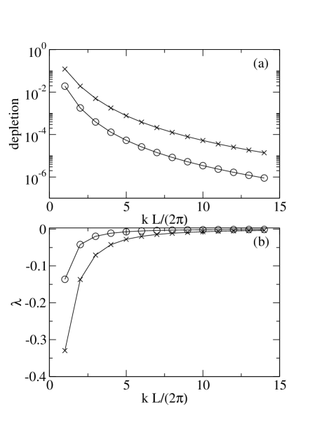
Figure 1: Panel (a) presents condensate depletion, i.e. number of atoms depleted from a condensate wavefunction, $dN_{k}^{a,b}=\left(v_{k,+}^{a,b}\right)^{2}+\left(v_{k,-}^{a,b}\right)^{2}$, to modes (44). Panel (b) shows the corresponding values of the parameters $\lambda_{k}^{a,b}$, Eqs. (49). Circles are related to the BEC component $a$ while crosses to the component $b$. The results correspond to the parameters far away from the phase separation, i.e. $N_{a}=5000$, $N_{b}=20000$, $L=50\;\mu$m, $a_{a}=108.8a_{0}$, $a_{b}=109.1a_{0}$ and $a_{ab}=10.0a_{0}$, where $a_{0}$ is the Bohr radius.

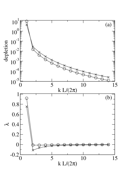
Figure 2: The same as Fig. 1 but for conditions close to the phase separation, i.e. $a_{ab}=193.9a_{0}$.

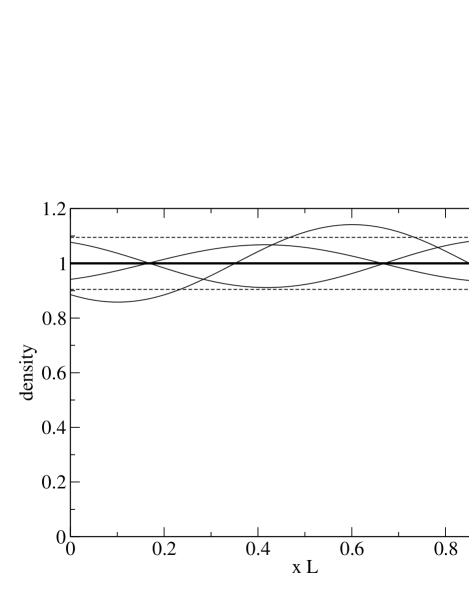
Figure 3: Solid curves show predictions for results of density measurements of atoms belonging to the $a$ component — the densities integrated over $y$ and $z$ directions, i.e. $L\int\sigma_{a}(\vec{r})\;dydz$, are shown. Thick solid line denotes the density averaged over many experimental realizations (i.e. the reduced single particle density) while dashed lines indicate the average density plus/minus standard deviation that is equal to $2\sqrt{\Lambda_{k}^{a}/N_{a}}\approx 0.1$ (where $k=2\pi/L$).

In Fig. 1 we show average numbers of atoms depleted to the modes (44) and values of the corresponding $\lambda^{a,b}_{k}$, Eqs. (49), far from the phase separation. The data correspond to a mixture of ⁸⁷Rb atoms in two different internal states, $N_{a}=5000$, $N_{b}=20000$, $L=50\;\mu$m, $a_{a}=108.8a_{0}$, $a_{b}=109.1a_{0}$ and $a_{ab}=10a_{0}$, where $a_{0}$ is the Bohr radius burke . The value of the latter scattering length can be adjusted by means of a Feshbach resonance timm98 . To obtain predictions for atomic density measurements one has to change phases of the modes, see (29), which in the present case of all negative $\lambda^{a,b}_{k}$ leads to

$$\varphi_{a\vec{k}s} = \phi_{a\vec{k}s}e^{-i{\rm Arg}(\lambda^{a}_{\alpha})/2}=i\phi_{a\vec{k}s},$$ (51)

$$\varphi_{b\vec{k}s} = \phi_{b\vec{k}s}e^{-i{\rm Arg}(\lambda^{b}_{\alpha})/2}=i\phi_{b\vec{k}s},$$ (52)

and similarly for the $\varphi_{a\vec{k}c}$ and $\varphi_{b\vec{k}c}$ modes. Due to the fact that $\phi_{a0}$ and $\phi_{b0}$ are real and all the $\varphi$ modes are purely imaginary we obtain, see (27),

$$\sigma_{a}(\vec{r}) \sim \phi^{2}_{a0}(\vec{r})+\frac{1}{N_{a}}\left|\sum_{\alpha=1}^{M_{a}}q_{a\alpha}\;\varphi_{a\alpha}(\vec{r})\right|^{2},$$ (53)

$$\sigma_{b}(\vec{r}) \sim \phi^{2}_{b0}(\vec{r})+\frac{1}{N_{b}}\left|\sum_{\alpha=1}^{M_{b}}q_{b\alpha}\;\varphi_{b\alpha}(\vec{r})\right|^{2}.$$ (54)

Because $q_{a\alpha}^{2}\sim{\Lambda^{a}_{\alpha}/2}$, $q_{b\alpha}^{2}\sim{\Lambda^{b}_{\alpha}}/2$ and $\Lambda^{a,b}_{\alpha}\ll N_{a,b}$ the density fluctuations turn out to be negligible, i.e. the density remains almost perfectly flat.

Figure 2 shows similar data as Fig. 1 but for $a_{ab}=193.9a_{0}$, i.e. chosen so that the phase separation condition in an infinite system would be already fulfilled but it is still not fulfilled in the case of the finite box. The numbers of atoms depleted are not dramatically greater than the ones in the case considered previously but now some values of $\lambda^{a,b}_{k}$ become positive. The latter has dramatic consequences for density fluctuations because the modes $\varphi$ corresponding to the positive $\lambda^{a,b}_{k}$ are real and their contributions to the atomic density are of order of $\sqrt{\Lambda^{a,b}_{\alpha}/N_{a,b}}$. Indeed, the predictions for atomic density measurements (neglecting contributions of order of $\Lambda^{a,b}_{\alpha}/N_{a,b}$) show that

$$\sigma_{a}(\vec{r}) \sim \phi^{2}_{a0}(\vec{r})+\frac{2\phi_{a0}(\vec{r})}{\sqrt{N_{a}}}{\sum_{\vec{k}}}^{\prime}\left[q_{a\vec{k}s}\varphi_{a\vec{k}s}(\vec{r})+q_{a\vec{k}c}\varphi_{a\vec{k}c}(\vec{r})\right],$$ (55)

$$\sigma_{b}(\vec{r}) \sim \phi^{2}_{b0}(\vec{r})+\frac{2\phi_{b0}(\vec{r})}{\sqrt{N_{b}}}{\sum_{\vec{k}}}^{\prime}\left[q_{b\vec{k}s}\varphi_{b\vec{k}s}(\vec{r})+q_{b\vec{k}c}\varphi_{b\vec{k}c}(\vec{r})\right],$$ (56)

where ${\sum_{\vec{k}}}^{\prime}$ runs over modes corresponding to positive $\lambda^{a,b}_{k}$ only. In each experimental realization one has to choose $q_{a\vec{k}s}$, $q_{a\vec{k}c}$, $q_{b\vec{k}s}$ and $q_{b\vec{k}c}$ randomly according to the probability density (30). In Fig. 3 we show a few examples of the simulations for atoms belonging to the $a$ component together with the averaged result (which corresponds to the reduced single particle density) — the figure presents the densities integrated over $y$ and $z$ directions. Despite the small number of atoms depleted to the lowest momentum mode ($\sim 0.3\%$) the changes of the density are of order of 10%. Standard deviations of the largest scale density fluctuations (i.e. corresponding to the quasi-particles with the momentum $k=2\pi/L$) behave like

$$\sqrt{\frac{\Lambda^{a,b}_{k}}{N_{a,b}}}\sim\frac{1}{\left(a_{ab}^{\rm c}-a_{ab}\right)^{1/4}},$$ (58)

where $a_{ab}^{\rm c}$ is the critical value for the phase separation. Exactly at the critical point the Bogoliubov theory breaks down, which is indicated e.g. by the divergence of the fluctuations in Eq. (58). For the parameters chosen in Fig. 2-3 we are, however, sufficiently far away from the critical point so that the predictions on the basis of the Bogoliubov theory are reliable.

From the experimental point of view it is important that the density fluctuates on a scale of the order of $L$. One may use low resolution in the density measurements so that statistical fluctuations will be practically eliminated and the only density modulations will correspond to the fluctuations considered here.

In the example considered, the range of $a_{ab}$ where one deals with positive $\lambda^{a,b}_{k}$ is about 10$\times$Bohr radius, which should be wide enough to enable experiments with the density fluctuations (58).

Note that the structure of the Bogoliubov vacuum state (LABEL:finalhomo) shows that there are no correlations between atoms belonging to the different components. Recently in Ref. jaksch , Bogoliubov vacuum of the form of (20) has been used in a two component system in the case when the inter-species interaction is absent, $g=0$, and the components become fully independent. Our analysis indicates that the Bogoliubov vacuum possesses the same form even in the presence of the inter-species interaction. Of course, the interaction changes the Bogoliubov modes and influences the values of $\lambda_{\alpha}^{a,b}$.

V Double well

In the present section we will consider a simple model where there are analytical solutions within the Bogoliubov theory both in the miscible and in the phase separated regime.

Let us consider a two component Bose-Einstein condensate in a one-dimensional symmetric double well potential under an assumption that the Hilbert space of the system is restricted to ground states in each well only (i.e. within the two mode approximation). For experimental realizations of the double well problem see dwell . The Hamiltonian of the system, if we choose real functions as the ground states in the two wells, reads

$$\hat{H} = -\frac{\Omega}{2}\left(\hat{A}_{1}^{\dagger}\hat{A}_{2}+\hat{A}_{2}^{\dagger}\hat{A}_{1}+\hat{B}_{1}^{\dagger}\hat{B}_{2}+\hat{B}_{2}^{\dagger}\hat{B}_{1}\right)$$ (61)

$$+\frac{U}{2}\left[\left(\hat{A}_{1}^{\dagger}\hat{A}_{1}\right)^{2}+\left(\hat{A}_{2}^{\dagger}\hat{A}_{2}\right)^{2}+\left(\hat{B}_{1}^{\dagger}\hat{B}_{1}\right)^{2}+\left(\hat{B}_{2}^{\dagger}\hat{B}_{2}\right)^{2}\right]$$

$$+U_{ab}\left(\hat{A}_{1}^{\dagger}\hat{A}_{1}\hat{B}_{1}^{\dagger}\hat{B}_{1}+\hat{A}_{2}^{\dagger}\hat{A}_{2}\hat{B}_{2}^{\dagger}\hat{B}_{2}\right),$$

where the $\hat{A}_{1}$ ($\hat{B}_{1}$) operator annihilates an atom belonging to the component $a$ ($b$) in the first well and the $\hat{A}_{2}$ ($\hat{B}_{2}$) operator annihilates an atom of the $a$ ($b$) component in the other well. For the calculations we have chosen potential wells situated at $x=-2,2$ and with such widths that the ground states of the wells are

$$\psi_{1}(x) = \left(\frac{2}{\pi}\right)^{1/4}e^{-(x+2)^{2}},$$ (62)

$$\psi_{2}(x) = \left(\frac{2}{\pi}\right)^{1/4}e^{-(x-2)^{2}}.$$ (63)

The parameter $\Omega$ stands for the frequency of the tunneling of atoms between the two wells and $U$ and $U_{ab}$ describe intra- and inter-condensate interactions. We will consider the case of symmetric BEC components, i.e. $N\equiv N_{a}=N_{b}=1000$, $\Omega=5000$, $U=1$ and $U_{ab}>0$ (i.e. all interactions are of repulsive nature), but similar analysis can be easily performed for $N_{a}\neq N_{b}$ and for tunneling frequencies and intra-species interactions different for both components.

We would like to mention that in the limit of large attractive interactions a two-component entanglement has been found in the system twocom2w .

V.1 Mean field solutions

For $U_{ab}$ smaller than the critical value

$$U^{c}_{ab}=\frac{\Omega}{N}+U,$$ (64)

the ground state solution of the Gross-Pitaevskii equations (10) reveals both condensates symmetrically located in the double well potential:

$$\phi_{a0}(x)=\phi_{b0}(x)=\frac{1}{\sqrt{2}}\left[\psi_{1}(x)+\psi_{2}(x)\right],$$ (65)

i.e. we are in the miscible regime. However, if the parameters of the system fulfil $U_{ab}>U^{c}_{ab}$ the solution (65) is unstable – the spatial overlap of the atomic clouds of the different components becomes energetically not favorable (see Fig. 4a) and the phase separation begins. The condensate wavefunctions are then:

$$\phi_{a0}(x) = \alpha\psi_{1}(x)+\beta\psi_{2}(x),$$ (66)

$$\phi_{b0}(x) = \beta\psi_{1}(x)+\alpha\psi_{2}(x),$$ (67)

where

$$\alpha = \sqrt{\frac{1+\sqrt{1-\gamma^{2}}}{2}},$$ (68)

$$\beta = \sqrt{\frac{1-\sqrt{1-\gamma^{2}}}{2}},$$ (69)

and

$$\gamma\equiv\frac{\Omega}{N(U_{ab}-U)}.$$ (70)

Note that in the phase separation regime there are two ground state solutions, for exchanging $\alpha\leftrightarrow\beta$ in (67) one obtains another solution of the Gross-Pitaevskii equations. On the basis of these two solutions two different Bogoliubov vacuum states can be obtained. In the following we will show that sufficiently far away from the critical point the ground state of the system can be approximated by preparing a superposition of the two Bogoliubov vacuum states.

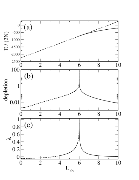
Figure 4: Panel (a): dashed line shows mean field energy of the symmetric Gross-Pitaevskii solution (65) while solid line denotes the energy of the asymmetric solution (67) which appears in the phase separation region. Panel (b) shows depletion of the condensates while panel (c) the corresponding values of $\lambda^{a,b}$. Note that, since we consider symmetric interactions, the depletions are equal for both components and $\lambda^{a}=\lambda^{b}$.

V.2 The Bogoliubov vacuum – miscible regime

The solution of the Bogoliubov-de Gennes equations reveals two quasi-particles corresponding to energies:

$$E_{\pm} = \left[\Omega\left(\Omega+NU\pm NU_{ab}\right)\right]^{1/2},$$ (71)

and modes:

$$\left(\begin{array}[]{c}u^{a}_{\pm}(x)\\ v^{a}_{\pm}(x)\\ u^{b}_{\pm}(x)\\ v^{b}_{\pm}(x)\end{array}\right)=\left(\begin{array}[]{c}(\Omega+2E_{\pm})\phi_{a1}(x)\\ (2E_{\pm}-\Omega)\phi_{a1}(x)\\ (\Omega+2E_{\pm})\phi_{b1}(x)\\ (2E_{\pm}-\Omega)\phi_{b1}(x)\end{array}\right)\chi_{\pm},$$ (72)

where

$$\phi_{a1}(x)=\phi_{b1}(x)=\frac{1}{\sqrt{2}}\left[\psi_{1}(x)-\psi_{2}(x)\right]$$ (73)

and

$$\chi_{\pm}=\frac{1}{4\sqrt{\Omega E_{\pm}}},$$ (74)

is the normalization factor.

The Bogoliubov vacuum state can be written in the form (20) using

$$\lambda^{a}=\lambda^{b}=\frac{\left(4E^{2}_{+}-\Omega^{2}\right)\chi^{2}_{+}+\left(4E^{2}_{-}-\Omega^{2}\right)\chi^{2}_{-}}{1+(2E_{+}-\Omega)^{2}\chi^{2}_{+}+(2E_{-}-\Omega)^{2}\chi^{2}_{-}}.$$ (75)

The parameters (75) and the depletion are shown versus $U_{ab}$ in Fig. 4.

As can be seen from the quasiparticle excitation energy (71), when the condition $U_{ab}>U^{c}_{ab}$ is fulfilled, the spectrum is no longer real and the solution (65) becomes unstable. The ground state of the Gross-Pitaevskii equations shows separation of the atomic clouds of the $a$ and $b$ components.

V.3 The Bogoliubov vacuum – phase separation regime

Now the quasi-particle excitation energies are

$$E_{\pm}=\left\{\frac{\Omega}{2}\left[\frac{\Omega}{2}\left(\frac{\alpha}{\beta}+\frac{\beta}{\alpha}\right)^{2}+4U\alpha\beta\right]\pm 2\Omega U_{ab}\alpha\beta\right\}^{1/2},$$ (76)

and the quasiparticle modes, corresponding to the condensate wavefunctions (67), are proportional to

$$\phi_{a1}(x) = \beta\psi_{1}(x)-\alpha\psi_{2}(x),$$ (78)

$$\phi_{b1}(x) = \alpha\psi_{1}(x)-\beta\psi_{2}(x).$$ (79)

We skip here rather long expressions for the quasiparticles since they can be easily obtained with the help of the Bogoliubov transformation. Behaviour of the component $a$ (or $b$) depletion and of the parameters $\lambda^{a},\lambda^{b}$ versus $U_{ab}$ is depicted in Fig. 4.

A Hamiltonian of a BEC system in a symmetric double well potential is invariant under the parity inversion, i.e. if we reverse coordinates of all particles the Hamiltonian does not change. It implies that eigenstates of our system (unless there is a degeneracy) must be also eigenstates of the parity operator. In the phase separation regime the Gross-Pitaevskii solutions (67) are neither even nor odd functions and the corresponding Bogoliubov vacuum,

$$|0_{B}\rangle \sim \left[\left(\hat{a}_{0}^{\dagger}\right)^{2}+\lambda^{a}\left(\hat{a}_{1}^{\dagger}\right)^{2}\right]^{N/2}$$ (81)

$$\times\left[\left(\hat{b}_{0}^{\dagger}\right)^{2}+\lambda^{b}\left(\hat{b}_{1}^{\dagger}\right)^{2}\right]^{N/2}|0\rangle,$$

is not an eigenstate of the parity operator. Exchanging $\alpha$ with $\beta$ one obtains another Gross-Pitaevskii solution and another Bogoliubov vacuum state. A proper parity state can be obtained by preparing a superposition of the two states

$$|0_{B}\rangle+|0_{B}({\alpha\leftrightarrow\beta})\rangle.$$ (82)

The state (82) is a good approximation for the ground state of the system if we are not very close to the critical point. That is, if we increase $U_{ab}$ for fixed $N$, the states $|0_{B}\rangle$ and $|0_{B}({\alpha\leftrightarrow\beta})\rangle$ very quickly become practically orthogonal, and the sooner it takes place, the greater $N$ we choose. Note that even in the regime of these states being orthogonal, the corresponding mean field states (67) need not be orthogonal at all. If we are, however, far away from the critical point also the Gross-Pitaevskii solutions have zero overlap, i.e. $\langle\phi_{a0}|\phi_{b0}\rangle\approx 0$. Then the state (82) is a a Schrödinger cat state schcat which is strongly vulnerable to atomic losses — loss of a small number of atoms is sufficient to distort completely the coherent superposition in (82).

At the critical point the Bogoliubov theory breaks down because higher order terms become dominant.

V.4 Density fluctuations

We see in Fig. 4 that approaching the critical point in the miscible regime the depletion of the condensates and the Bogoliubov vacuum parameters $\lambda^{a(b)}$ grow. Very close to the critical point the depletion is very large and the Bogoliubov theory can not be longer applied. However, in the vicinity of the point there is a regime where the depletions are very small compared to the total particle numbers and the parameters $\lambda^{a(b)}$ are positive. The modes $\phi_{a0}$, $\phi_{b0}$, $\phi_{a1}$ and $\phi_{b1}$ are real and the appearance of the positive $\lambda^{a,b}$ indicates (similarly as in the previous section) that density fluctuations become considerable, i.e. of order of $\sqrt{\Lambda^{a,b}/N}$,

$$\sigma_{a}(x) \sim \phi^{2}_{a0}(x)+2\frac{q_{a}}{\sqrt{N}}\phi_{a0}(x)\phi_{a1}(x),$$ (83)

$$\sigma_{b}(x) \sim \phi^{2}_{b0}(x)+2\frac{q_{b}}{\sqrt{N}}\phi_{b0}(x)\phi_{b1}(x),$$ (84)

where $q_{a}$ and $q_{b}$ have to be chosen randomly according to (30) in order to get predictions for the results of the density measurement in different experimental realizations.

A few examples of the density measurements of the $a$ component atoms in the miscible regime are shown in Fig. 5 for $U_{ab}^{\rm c}-U_{ab}=0.005$. Standard deviations of the density fluctuations behave like:

$$\sqrt{\frac{\Lambda^{a}}{N}}\sim\frac{1}{\left(U_{ab}^{\rm c}-U_{ab}\right)^{1/4}},$$ (86)

i.e. similarly as in the homogeneous case, see (58).

On the other side of the critical point, i.e. in the phase separation regime, we deal with a state of the form (82) which for $U_{ab}^{\rm c}-U_{ab}=-0.005$ and $N=5000$ is a good approximation for the ground state of the system, indeed $|\langle 0_{B}|0_{B}({\alpha\leftrightarrow\beta})\rangle|^{2}$ is of order of $10^{-8}$. One may also expect (similarly as in the miscible regime) substantial density fluctuations. However, for a superposition of the Bogoliubov vacuum states (82) we cannot simulate density measurements with the help of the method described in Sec. III.

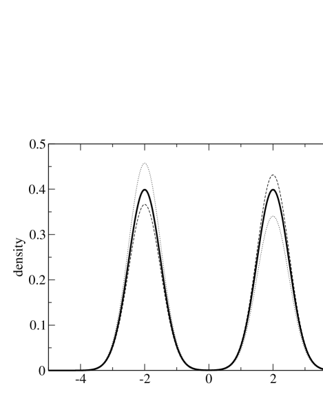
Figure 5: Density fluctuations of the $a$ component in the miscible regime close to the critical point, i.e. for $U_{ab}=5.995$. Solid line corresponds to the mean field solution, dashed and dotted lines are two examples of possible realizations of the experiment. The standard deviation of the density fluctuation is $\sqrt{2\Lambda^{a}/N}\phi_{a0}\phi_{a1}\approx 0.09\phi_{a0}\phi_{a1}$.

VI Conclusions

We have considered a number conserving version of the Bogoliubov theory for a two component Bose-Einstein condensate, with the fixed number of atoms in each component. We have shown that the Bogoliubov vacuum state can be written in the particle representation in a simple form, provided that eigenstates of the reduced single particle density matrices diagonalize the operators (24). Having the Bogoliubov vacuum in the particle representation one can easily obtain predictions for density measurements in single experiments.

The introduced formalism has been applied to the analysis of a two component homogeneous condensate and a two component condensate in a double well potential. In finite homogeneous systems, when parameters of the system approach a phase separation condition, considerable density fluctuations appear before the system becomes unstable. This behaviour is different than in infinite systems, where the phase separation happens abruptly. The range of the parameter values where the substantial fluctuations are observed indicates that the results presented here can be verified experimentally.

In the case of condensates in a double well potential we are able to describe the system in a vicinity of the critical point both in the miscible condensates regime and in the phase separation region. Considerable density fluctuations can be expected if the parameters approach the critical values.

Appendix A

We begin with a short reminder of the results of the number conserving version of the Bogoliubov theory. Following sorensen we will perform the perturbation expansion of the hamiltonian. The decomposition (8) allows us to expand the Hamiltonian in powers of small operators $\delta\hat{\psi}_{a}$ and $\delta\hat{\psi}_{b}$. As mentioned in Sec. II, minimizing the energy of the system in the zero order we obtain coupled Gross-Pitaevskii equations (10) that allow us to find the condensate wavefunctions $\phi_{a0}$ and $\phi_{b0}$. The first order terms of the Hamiltonian disappear and in the second order we obtain an effective Hamiltonian

$$\hat{H}_{\rm eff}\approx\frac{1}{2}\int d^{3}r\left(\hat{\Lambda}_{a}^{\dagger},-\hat{\Lambda}_{a},\hat{\Lambda}_{b}^{\dagger},-\hat{\Lambda}_{b}\right){\cal L}\left(\begin{array}[]{c}\hat{\Lambda}_{a}\\ \hat{\Lambda}_{a}^{\dagger}\\ \hat{\Lambda}_{b}\\ \hat{\Lambda}_{b}^{\dagger}\end{array}\right),$$ (A-1)

where

$${\cal L}=\left(\begin{array}[]{cccc}H_{GP}^{a}+g_{a}N_{a}\hat{Q}_{a}|\phi_{a0}|^{2}\hat{Q}_{a}&g_{a}N_{a}\hat{Q}_{a}\phi_{a0}^{2}\hat{Q}_{a}^{*}&g\sqrt{N_{a}N_{b}}Q_{a}\phi_{a0}\phi^{*}_{b0}Q_{b}&g\sqrt{N_{a}N_{b}}Q_{a}\phi_{a0}\phi_{b0}Q^{*}_{b}\\ -g_{a}N_{a}\hat{Q}^{*}_{a}\phi_{a0}^{*2}\hat{Q}_{a}&-H_{GP}^{a}-g_{a}N_{a}\hat{Q}^{*}_{a}|\phi_{a0}|^{2}\hat{Q}^{*}_{a}&-g\sqrt{N_{a}N_{b}}Q^{*}_{a}\phi^{*}_{a0}\phi^{*}_{b0}Q_{b}&-g\sqrt{N_{a}N_{b}}Q^{*}_{a}\phi^{*}_{a0}\phi_{b0}Q^{*}_{b}\\ g\sqrt{N_{a}N_{b}}Q_{b}\phi^{*}_{a0}\phi_{b0}Q_{a}&g\sqrt{N_{a}N_{b}}Q_{b}\phi_{a0}\phi_{b0}Q^{*}_{a}&H_{GP}^{b}+g_{b}N_{b}\hat{Q}_{b}|\phi_{b0}|^{2}\hat{Q}_{b}&g_{b}N_{b}\hat{Q}_{b}\phi_{b0}^{2}\hat{Q}_{b}^{*}\\ -g\sqrt{N_{a}N_{b}}Q^{*}_{b}\phi^{*}_{a0}\phi^{*}_{b0}Q_{a}&-g\sqrt{N_{a}N_{b}}Q^{*}_{b}\phi_{a0}\phi^{*}_{b0}Q^{*}_{a}&-g_{b}N_{b}\hat{Q}^{*}_{b}\phi_{b0}^{*2}\hat{Q}_{b}&-H_{GP}^{b}-g_{b}N_{b}\hat{Q}^{*}_{b}|\phi_{b0}|^{2}\hat{Q}^{*}_{b}\\ \end{array}\right),$$ (A-2)

and

$$\hat{Q}_{a} = 1-|\phi_{a0}\rangle\langle\phi_{a0}|,$$ (A-3)

$$\hat{Q}_{b} = 1-|\phi_{b0}\rangle\langle\phi_{b0}|.$$ (A-4)

The $\hat{\Lambda}_{a}(\vec{r})$ and $\hat{\Lambda}_{b}(\vec{r})$ operators (17) fulfil the following commutation relations

$$[\hat{\Lambda}_{a}(\vec{r}),\hat{\Lambda}_{a}^{\dagger}(\vec{r}\;^{\prime})]\approx\langle\vec{r}|\hat{Q}_{a}|\vec{r}\;^{\prime}\rangle,$$ (A-5)

$$[\hat{\Lambda}_{b}(\vec{r}),\hat{\Lambda}_{b}^{\dagger}(\vec{r}\;^{\prime})]\approx\langle\vec{r}|\hat{Q}_{b}|\vec{r}\;^{\prime}\rangle.$$ (A-6)

Note that action of the $\hat{\Lambda}_{a}$ and $\hat{\Lambda}_{b}$ operators preserves numbers of atoms in the system. Diagonalization of the effective Hamiltonian amounts to solving the eigen-equation for the non-hermitian operator $\cal L$ (i.e. the Bogoliubov-de Gennes equations).

The $\cal L$ operator possesses two symmetries (similarly to the symmetries of the original Bogoliubov-de Gennes equations castin ),

$$u_{1}{\cal L}u_{1} = -{\cal L}^{*},$$ (A-7)

$$u_{3}{\cal L}u_{3} = {\cal L}^{\dagger},$$ (A-8)

where

$$u_{1}=\left(\begin{array}[]{c|c}\sigma_{1}&0\\ \hline\cr 0&\sigma_{1}\\ \end{array}\right), u_{3}=\left(\begin{array}[]{c|c}\sigma_{3}&0\\ \hline\cr 0&\sigma_{3}\\ \end{array}\right),$$ (A-13)

and

$$\sigma_{1}=\left(\begin{array}[]{cc}0&1\\ 1&0\end{array}\right), \sigma_{3}=\left(\begin{array}[]{cc}1&0\\ 0&-1\end{array}\right),$$ (A-18)

are the first and third Pauli matrices, respectively. Suppose that all eigenvalues of the ${\cal L}$ operator are real. The symmetries (A-8) imply that if

$$|\Psi_{n}^{\rm R}\rangle=\left(\begin{array}[]{c}|u_{n}^{a}\rangle\\ |v_{n}^{a}\rangle\\ |u_{n}^{b}\rangle\\ |v_{n}^{b}\rangle\\ \end{array}\right),$$ (A-19)

is a right eigenvector of the ${\cal L}$ with eigenvalue $E_{n}$, then $|\Psi_{n}^{\rm L}\rangle=u_{3}|\Psi_{n}^{\rm R}\rangle$ is a left eigenvector of the same eigenvalue $E_{n}$, and $u_{1}|\Psi^{R\ast}_{n}\rangle$ is a right eigenvector with eigenvalue $-E_{n}$.

There are four eigenvectors of ${\cal L}$ corresponding to a zero eigenvalue,

$$\left(\begin{array}[]{c}|\phi_{a}\rangle\\ 0\\ 0\\ 0\\ \end{array}\right),\;\left(\begin{array}[]{c}0\\ |\phi_{a}^{*}\rangle\\ 0\\ 0\\ \end{array}\right),\;\left(\begin{array}[]{c}0\\ 0\\ |\phi_{b}\rangle\\ 0\\ \end{array}\right),\;\left(\begin{array}[]{c}0\\ 0\\ 0\\ |\phi_{b}^{*}\rangle\\ \end{array}\right).$$ (A-36)

The other eigenstates of the ${\cal L}$ operator we divide into two families ”+” and ”$-$”, according to

$$\langle\Psi_{n}^{\rm R}|u_{3}|\Psi_{n^{\prime}}^{\rm R}\rangle=\pm\delta_{n,n^{\prime}}.$$ (A-37)

Having the complete set of the eigenvectors of the $\cal L$ we obtain an important completeness relation

$$\hat{1} = \sum_{n\in"+"}\left(\begin{array}[]{c}|u_{n}^{a}\rangle\\ |v_{n}^{a}\rangle\\ |u_{n}^{b}\rangle\\ |v_{n}^{b}\rangle\end{array}\right)\left(\langle u_{n}^{a}|,-\langle v_{n}^{a}|,\langle u_{n}^{b}|,-\langle v_{n}^{b}|\right)+\sum_{n\in"+"}\left(\begin{array}[]{c}|v_{n}^{a*}\rangle\\ |u_{n}^{a*}\rangle\\ |v_{n}^{b*}\rangle\\ |u_{n}^{b*}\rangle\end{array}\right)\left(-\langle v_{n}^{a*}|,\langle u_{n}^{a*}|,-\langle v_{n}^{b*}|,\langle u_{n}^{b*}|\right)$$ (A-51)

$$+\left(\begin{array}[]{cccc}|\phi_{a0}\rangle\langle\phi_{a0}|&0&0&0\\ 0&|\phi_{a0}^{*}\rangle\langle\phi_{a0}^{*}|&0&0\\ 0&0&|\phi_{b0}\rangle\langle\phi_{b0}|&0\\ 0&0&0&|\phi_{b0}^{*}\rangle\langle\phi_{b0}^{*}|\\ \end{array}\right).$$

The eigenvectors of the $\cal L$ operator define the Bogoliubov transformation

$$\left(\begin{array}[]{c}\hat{\Lambda}_{a}\\ \hat{\Lambda}_{a}^{\dagger}\\ \hat{\Lambda}_{b}\\ \hat{\Lambda}_{b}^{\dagger}\end{array}\right)=\sum_{n\in"+"}\left(\begin{array}[]{c}u_{n}^{a}\\ v_{n}^{a}\\ u_{n}^{b}\\ v_{n}^{b}\end{array}\right)\hat{c}_{n}+\sum_{n\in"+"}\left(\begin{array}[]{c}v_{n}^{a*}\\ u_{n}^{a*}\\ v_{n}^{b*}\\ u_{n}^{b*}\end{array}\right)\hat{c}_{n}^{\dagger},$$ (A-52)

where the quasi-particle operators (15) fulfill the bosonic commutation relation $[\hat{c}_{n},\hat{c}^{\dagger}_{n^{\prime}}]\approx\delta_{n,n^{\prime}}$. Employing the Bogoliubov transformation we obtain the effective Hamiltonian in a diagonal form (14).

Appendix B

The Bogoliubov vacuum state $|0_{B}\rangle$ is an eigenstate of the effective Hamiltonian (14) that is annihilated by all quasi-particle annihilation operators. Let us show that the Bogoliubov vacuum can be obtained from the particle vacuum by applying some particle creation operators $\hat{d}_{a}^{\dagger}$ and $\hat{d}_{b}^{\dagger}$

$$|0_{B}\rangle\sim\left(\hat{d}_{a}^{\dagger}\right)^{M_{a}}\left(\hat{d}_{b}^{\dagger}\right)^{M_{b}}|0\rangle,$$ (B-1)

where we require that $\hat{d}_{a}^{\dagger}$ and $\hat{d}_{b}^{\dagger}$ commute with all quasi-particle annihilation operators dziarmaga ,

$$[\hat{c}_{n},\hat{d}_{a}^{\dagger}] = 0,$$ (B-2)

$$[\hat{c}_{n},\hat{d}_{b}^{\dagger}] = 0.$$ (B-3)

Then the state (B-1) is indeed annihilated by all quasi-particle annihilation operators,

$$\hat{c}_{n}\left(\hat{d}_{a}^{\dagger}\right)^{M_{a}}\left(\hat{d}_{b}^{\dagger}\right)^{M_{b}}|0\rangle=\left(\hat{d}_{a}^{\dagger}\right)^{M_{a}}\left(\hat{d}_{b}^{\dagger}\right)^{M_{b}}\hat{c}_{n}|0\rangle=0.$$ (B-4)

The set of equations (B-3) is solved by the particle creation operators in the form dziarmaga ; ansatzL

$$\hat{d}_{a}^{\dagger} = \hat{a}_{0}^{\dagger}\hat{a}_{0}^{\dagger}+\sum_{\alpha,\beta=1}^{\infty}Z_{\alpha\beta}^{a}\hat{a}_{\alpha}^{\dagger}\hat{a}_{\beta}^{\dagger}$$ (B-5)

$$\hat{d}_{b}^{\dagger} = \hat{b}_{0}^{\dagger}\hat{b}_{0}^{\dagger}+\sum_{\alpha,\beta=1}^{\infty}Z_{\alpha\beta}^{b}\hat{b}_{\alpha}^{\dagger}\hat{b}_{\beta}^{\dagger},$$ (B-6)

where $\hat{a}_{\alpha}^{\dagger}$ ($\hat{b}_{\alpha}^{\dagger}$) are bosonic particle creation operators that create atoms in modes $\phi_{a\alpha}$ ($\phi_{b\alpha}$) orthogonal to the condensate wavefunction $\phi_{a0}$ ($\phi_{b0}$). $Z_{\alpha\beta}^{a}$ and $Z_{\alpha\beta}^{b}$ are symmetric matrices to be found.

Substituting the ansatz (B-6) into (B-3) we obtain equations:

$$\langle v_{n}^{a}|\phi_{a\alpha}^{*}\rangle = \sum_{\beta=1}^{\infty}\langle u_{n}^{a}|\phi_{a\beta}\rangle Z_{\beta\alpha}^{a}$$ (B-7)

$$\langle v_{n}^{b}|\phi_{b\alpha}^{*}\rangle = \sum_{\beta=1}^{\infty}\langle u_{n}^{b}|\phi_{b\beta}\rangle Z_{\beta\alpha}^{b},$$ (B-8)

which, when multiplied by $\langle\phi_{a\gamma}|u_{n}^{a}\rangle$ and $\langle\phi_{b\gamma}|u_{n}^{b}\rangle$, respectively, and summed over $n$, are transformed to

$$\langle\phi_{a\gamma}|\hat{\Gamma}_{a}|\phi_{a\alpha}^{*}\rangle = \sum_{\beta=1}^{\infty}\langle\phi_{a\gamma}|\hat{U}_{a}|\phi_{a\beta}\rangle Z_{\beta\alpha}^{a}$$ (B-9)

$$\langle\phi_{b\gamma}|\hat{\Gamma}_{b}|\phi_{b\alpha}^{*}\rangle = \sum_{\beta=1}^{\infty}\langle\phi_{b\gamma}|\hat{U}_{b}|\phi_{b\beta}\rangle Z_{\beta\alpha}^{b},$$ (B-10)

where

$$\hat{U}_{a}=\sum_{n\in"+"}|u_{n}^{a}\rangle\langle u_{n}^{a}|,\quad\hat{U}_{b}=\sum_{n\in"+"}|u_{n}^{b}\rangle\langle u_{n}^{b}|,$$ (B-11)

and $\hat{\Gamma}_{a,b}$ are defined in (24). The completeness relation (A-51) implies that the $\hat{\Gamma}_{a}$ and $\hat{\Gamma}_{b}$ operators are symmetric and that

$$\hat{U}_{a} = \sum_{n\in"+"}|v_{n}^{a*}\rangle\langle v_{n}^{a*}|+\hat{1}_{\perp}^{a},$$ (B-12)

$$\hat{U}_{b} = \sum_{n\in"+"}|v_{n}^{b*}\rangle\langle v_{n}^{b*}|+\hat{1}_{\perp}^{b},$$ (B-13)

where $\hat{1}_{\perp}^{a}$ and $\hat{1}_{\perp}^{b}$ are the identity operators in the subspaces orthogonal to the condensate wavefunctions $\phi_{a0}$ and $\phi_{b0}$, respectively. Comparing Eq. (B-12) with

$$\langle 0_{B}|\hat{\psi}_{a}^{\dagger}(\vec{r})\hat{\psi}_{a}(\vec{r}\;^{\prime})|0_{B}\rangle = N_{a}\phi_{a0}^{*}(\vec{r})\phi_{a0}(\vec{r}\;^{\prime})$$ (B-15)

$$+\sum_{n\in"+"}v_{n}^{a}(\vec{r})v_{n}^{a*}(\vec{r}\;^{\prime}).$$

we see that the $\hat{U}_{a}$ operator is a sum of a part of the reduced single particle density operator corresponding to the subspace orthogonal to the condensate wavefunction $\phi_{a0}$ and the identity operator $\hat{1}_{\perp}^{a}$. Similar statement is true in the case of the $b$ component. Thus, if we choose as a basis $\phi_{a\alpha}$ ($\phi_{b\alpha}$), the eigenstates of the single particle density matrix, we get the $\hat{U}_{a}$ ($\hat{U}_{b}$) operator in a diagonal form. Then one obtains immediately the solutions for the $Z^{a,b}_{\alpha\beta}$ matrices, i.e.

$$Z_{\alpha\beta}^{a}=\frac{\langle\phi_{a\alpha}|\hat{\Gamma}_{a}|\phi_{a\beta}^{*}\rangle}{dN^{a}_{\alpha}+1},\quad Z_{\alpha\beta}^{b}=\frac{\langle\phi_{b\alpha}|\hat{\Gamma}_{b}|\phi_{b\beta}^{*}\rangle}{dN^{b}_{\alpha}+1},$$ (B-16)

where $dN_{\alpha}^{a,b}$ are the eigenvalues of the single particle density matrices, that is numbers of atoms depleted from the condensate wavefunctions to other eigenmodes. The $Z^{a}_{\alpha\beta}$, $Z^{b}_{\alpha\beta}$, $\langle\phi_{a\alpha}|\hat{\Gamma}_{a}|\phi_{a\beta}^{*}\rangle$ and $\langle\phi_{b\alpha}|\hat{\Gamma}_{b}|\phi_{b\beta}^{*}\rangle$ matrices are symmetric. Thus, in order the ansatz (B-6) to be self-consistent the $\hat{\Gamma}_{a,b}$ operators have to be also diagonal in the basis of the eigenvectors of the single particle density matrices. In Sec. IV and V we show examples where indeed this is the case. Final form of the solution for the Bogoliubov vacuum state in the particle representation is presented in (20).

References

- (1) Bose-Einstein Condensation in Atomic Gases, Proceedings of the International School of Physics “Enrico Fermi”, course 140, edited by M. Inguscio, S. Stringari, and C. Wieman (IOS Press, Amsterdam, 1999).
- (2) C. J. Myatt, E. A. Burt, R. W. Ghrist, E. A. Cornell, C. E. Wieman, Phys. Rev. Lett. 78, 586 (1997); D. S. Hall, M. R. Matthews, C. E. Wieman, E. A. Cornell, Phys. Rev. Lett. 81, 1543 (1998); J. Stenger, S. Inouye, D. M. Stamper-Kurn, H. J. Miesner, A. P. Chikkatur, W. Ketterle, Nature 396, 345 (1998); G. Modugno, M. Modugno, F. Riboli, G. Roati, and M. Inguscio, Phys. Rev. Lett. 89, 190404 (2002).
- (3) B. D. Esry, C. H. Greene, J. P. Burke, J. T. Bohn, Phys. Rev. Lett. 78, 3594 (1997); M. Trippenbach, K. Góral, K. Rza̧żewski, B. Malomed, Y. B. Band, J. Phys. B 33, 4017 (2000); F. Riboli and M. Modugno, Phys. Rev. A 65, 063614 (2002); A. A. Svidzinsky and S. T. Chui, Phys. Rev. A 67, 053608 (2003);
- (4) E. Timmermans, Phys. Rev. Lett. 81, 5718 (1998); A. S. Alexandrov, V. V. Kabanov, J. Phys.: Condens. Matter 14 L327 (2002); P. Ao and S. T. Chui, Phys. Rev. A 58, 4836 (1998).
- (5) F. M. Cucchietti and E. Timmermans, Phys. Rev. Lett. 96, 210401 (2006); R. M. Kalas and D. Blume, Phys. Rev. A 73, 043608 (2006); K. Sacha and E. Timmermans, Phys. Rev. A 73, 063604 (2006).
- (6) A. Sørensen, L.-M. Duan, J. I. Cirac and P. Zoller, Nature 409, 63 (2001).
- (7) A. S. Sørensen, Phys. Rev. A 65, 043610 (2002).
- (8) E. V. Goldstein and P. Meystre, Phys. Rev. A 55, 2935 (1997); C. P. Search, A. G. Rojo, and P. R. Berman, Phys. Rev. A 64, 013615 (2001); P. Tommasini, E. J. V. de Passos, A. F. R. de Toledo Piza, M. S. Hussein, and E. Timmermans, Phys. Rev. A 67, 023606 (2003).
- (9) L.P. Pitaevskii, Zh. Eksp. Teor. Fiz. 40, 646 (1961) [Sov. Phys.JETP 13, 451 (1961)]; E.P. Gross, Nuovo Cimento 20, 454 (1961); F. Dalfovo et al., Rev. Mod. Phys. 71, 463 (1999).
- (10) Ph. Nozieres and D. Pines, The Theory of Quantum Liquids, (Addison Wesley, New York, 1990), Vol.II; A.L. Fetter, Ann. Phys. (N.Y.), 70, 67 (1972).
- (11) Y. Castin and R. Dum, Phys. Rev. A 57, 3008 (1998); Y. Castin, in Les Houches Session LXXII, Coherent atomic matter waves 1999, edited by R. Kaiser, C. Westbrook and F. David, (Springer-Verlag Berlin Heilderberg New York 2001).
- (12) M. D. Girardeau and R. Arnowitt, Phys. Rev. 113, 755 (1959); C. W. Gardiner, Phys. Rev. A 56, 1414 (1997); M. D. Girardeau Phys. Rev. A 58, 775 (1998).
- (13) M. Lewenstein and L. You, Phys. Rev. Lett. 77, 3489 (1996).
- (14) J. Dziarmaga and K. Sacha, Phys. Rev. A 67, 033608 (2003).
- (15) J. Javanainen and S.Mi. Yoo, Phys. Rev. Lett. 76, 161 (1996).
- (16) J. Dziarmaga, Z. P. Karkuszewski and K. Sacha, J. Phys. B 36, 1217 (2003); J. Dziarmaga and K. Sacha, J. Phys. B 39, 57 (2006).
- (17) J. Chwedeńczuk, P. Ziń, K. Rza̧żewski, and M. Trippenbach, Phys. Rev. Lett. 97, 170404 (2006).
- (18) A. J. Leggett, Rev. Mod. Phys. 73, 307 (2001).
- (19) D. M. Larsen, Ann. Phys. (N.Y.) 24, 89 (1963); W. H. Bassichis, Phys. Rev. 134, A543 (1964); W.-J. Huang and S.-C. Gou, Phys. Rev. A 59, 4608 (1999).
- (20) J. P. Burke, Jr., J. L. Bohn, B. D. Esry, and C. H. Greene, Phys. Rev. A 55 R2511 (1997).
- (21) M. Rodríguez, S. R. Clark, and D. Jaksch, Phys. Rev. A 75, 011601 (2007).
- (22) M. R. Andrews, C. G. Townsend, H.-J. Miesner, D. S. Durfee, D. M. Kurn, W. Ketterle, Science 275, 637 (1997); Y. Shin, M. Saba, T. A. Pasquini, W. Ketterle, D. E. Pritchard, and A. E. Leanhardt, Phys. Rev. Lett. 92, 050405 (2004); M. Albiez, R. Gati, J. Fölling, S. Hunsmann, M. Cristiani, and M. K. Oberthaler, Phys. Rev. Lett. 95, 010402 (2005).
- (23) H. T. Ng, C. K. Law, and P. T. Leung, Phys. Rev. A 68, 013604 (2003); J. Chen, Y. Guo, H. Cao, and H. Song, arXiv:quant-ph/0507191.
- (24) J. I. Cirac, M. Lewenstein, K. Mølmer, and P. Zoller, Phys. Rev. A 57, 1208 (1998); J. Ruostekoski, M. J. Collett, R. Graham, and D. F. Walls, Phys. Rev. A 57, 511 (1998); D. Gordon and C. M. Savage, Phys. Rev. A 59, 4623 (1999); D. A. R. Dalvit, J. Dziarmaga, and W. H. Zurek, Phys. Rev. A 62, 013607 (2000).