Disorder effects in the quantum Heisenberg model: An Extended Dynamical mean-field theory analysis

Abstract

We investigate a quantum Heisenberg model with both antiferromagnetic and disordered nearest-neighbor couplings. We use an extended dynamical mean-field approach, which reduces the lattice problem to a self-consistent local impurity problem that we solve by using a quantum Monte Carlo algorithm. We consider both two- and three-dimensional antiferromagnetic spin fluctuations and systematically analyze the effect of disorder. We find that in three dimensions for any small amount of disorder a spin-glass phase is realized. In two dimensions, while clean systems display the properties of a highly correlated spin-liquid (where the local spin susceptibility has a non-integer power-low frequency and/or temperature dependence), in the present case this behavior is more elusive unless disorder is very small. This is because the spin-glass transition temperature leaves only an intermediate temperature regime where the system can display the spin-liquid behavior, which turns out to be more apparent in the static than in the dynamical susceptibility.

I Introduction

Quantum magnetism is an important topic of modern solid state physics: Not only do magnetic phases take place in the phase diagram of many correlated electron systems, like high-temperature superconducting cuprates reviewcuprates and heavy fermions reviewHF , but many different materials display magnetic properties, which change upon varying parameters such as doping, temperature, disorder, or pressure. A few examples may (very partially) illustrate the enormous variety of behaviors that one encounters in this field: Upon increasing doping the lightly doped ${\rm La_{2-x}Sr_{x}CuO_{4}}$ passes from an antiferromagnetic (AF) to a spin-glass (SG) phasereviewcuprates ; the introduction of non-magnetic impurities in quantum paramagnets like ${\rm SrCu_{2}O_{3}}$, ${\rm KCuCl_{3}}$, ${\rm CuGeO_{3}}$, gives rise to local-moment formationwebervojta ; the glassy phase of the disordered dipolar-coupled magnet ${\rm LiHo_{x}Y_{1-x}F_{4}}$ may be driven to other magnetic phases by means of a magnetic fieldLHYF ; ${\rm SrCr_{9p}Ga_{12-9p}O_{19}}$ is a $S=3/2$ magnet with a Kagomé lattice structure, which above the (low) SG freezing temperature displays the spin-liquid behavior notespin-liquid ; sachdevye typical of strongly correlated spin systemsmondelli . From this large variety we extract three essential ingredients, which are commonly and physically relevant in quantum magnetic materials: disorder, frustration, and fluctuations (both thermal and quantum). The separate role of these physical mechanisms and their interplay in determining different physical properties is obviously a relevant issue in the field of quantum magnetism. Since one is facing a huge variety of systems with different structures, properties and phase diagrams, the search of common fundamental mechanisms mostly relies on the analysis of schematic models to highlight the deep physical effects. For instance some work has been devoted to the interplay between disorder and fluctuations georgesparcollet ; rozenberg ; daniel-marcelo , analyzing the role of quantum spin fluctuations in driving a spin-glass (SG) phase into a paramagnetic (or spin-liquid) phase upon varying spin size and/or temperature. Within the same framework we consider in this paper a “simple” quantum AF Heisenberg model for $S=1/2$ spins and we introduce a random magnetic coupling. By solving this Disordered Quantum Antiferromagnetic Heisenberg (DQAFH) model within the Extended Dynamical Mean-Field Theory (EDMFT)smithsi ; chitrakotliar ; BGG , we aim to clarify the interplay between AF and random magnetic couplings as well as the role of dimensionality in the instability from a paramagnetic to a SG phase and the relevance of quantum fluctuations in suppressing the critical temperature. Throughout the present work we will always remain in the paramagnetic phase with neither AF- nor replica-symmetry breaking and we will determine the conditions for these (second-order) instabilities to take place.

The EDMFT technique smithsi ; chitrakotliar ; BGG is an extension of the standard Dynamical Mean-Field Theory reviewDMFT , where the local (spin or charge) degrees of freedom are coupled to a self-consistent bosonic bath. In our case the Heisenberg model is mapped onto a single quantum spin embedded in a bosonic bath which represents the surrounding spin excitations as a fluctuating magnetic field. This approach has some definite limitations: It is not suited to keep full account of the spin character of the surrounding degrees of freedom (for instance it misses the possibility of singlet formation between the single spin and the surrounding ones) and it neglects the momentum dependence of the spin self-energy thereby preventing the occurrence of spatial anomalous dimensions. This latter limitation is more severe at low temperatures, where spatial correlations between the spins become relevant. As also discussed in Section VI the consequence of this is the appearance of well-known BGG ; haule low-temperature instabilities occurring as an unphysical sign in the spin self-energy. Also related to this poor treatment of spatial correlations (and the related lack of anomalous dimensions) is the appearance of spurious first-order transitions, where second-order are instead expected PKM . Nevertheless, it is commonly recognized PKM that the EDMFT approach is a valuable tool to investigate the dynamics of spin systems and it makes an important first step toward the inclusion of spatial correlations between the spins.

Our analysis of the DQAFH not only has a broad validity and addresses general theoretical issues, but it is also of pertinence for those numerous AF materials, where disorder can induce competition between antiferromagnetism (possibly having a correlated anomalous character) and a spin glass (SG) phase, or can induce local moment formation with low-temperature Curie-like dependencies. The role of low dimensionality in determining the relevance of magnetic fluctuations is also investigated.

The paper is organized as follows. In Section II we present the model and the EDMFT technique. Section III presents the criteria necessary to detect the establishment of broken-symmetry phases or the spin-liquid behavior. The numerical results for static properties in the three- and two-dimensional case are reported in Section IV, while the dynamical behavior is discussed in Sect. V. In Section VI we discuss our results and present our conclusions.

II The model and the technique

II.1 The model

We consider the Disordered Quantum Antiferromagnetic Heisenberg (DQAFH) model, given by the following Hamiltonian:

$$H=\sum_{i<j}\tilde{J}_{ij}{\bf S}_{i}{\bf S}_{j}~{}.$$ (1)

Here ${\bf S}_{i}$ is a spin$-1/2$ operator at the $i-$th site of a lattice of coordination $z$. The nearest-neighbor magnetic couplings $\tilde{J}_{ij}\equiv\tilde{J}_{ij}^{AF}+\tilde{J}_{ij}^{D}$ are the sum of a translationally invariant part $\tilde{J}_{ij}^{AF}\equiv{J}_{ij}^{AF}/\sqrt{z}\equiv J/\sqrt{z}$ [with Fourier transforms $J({\bf q})$] and a disordered part $\tilde{J}_{ij}^{D}\equiv J_{ij}^{D}/\sqrt{z}$. The translationally invariant couplings are related to the spin-wave spectral density $\rho(\epsilon)\equiv\sum_{{\bf q}}\delta(\epsilon-J({\bf q}))$. The disordered parts $J_{ij}^{D}$ are random couplings with a Gaussian probability distribution $P(J_{ij}^{D})$, with zero mean value $\langle J_{ij}^{D}\rangle_{dis}=0$ and $\langle J_{ij}^{D}J_{kl}^{D}\rangle_{dis}=\delta_{i,l}\delta_{j,k}J_{D}^{2}$ [$\langle\cdots\rangle_{dis}$ represents the averaging over the disorder distribution].

In the following, we will perform a large-$z$ expansion, in order to study the spin-wave correlations within a single-site effective model. This derivation has been described in Ref. smithsi, for a clean Heisenberg model. Here, the presence of disorder requires a specific preliminary treatment.

II.1.1 Disorder and replicas

The free energy is averaged with respect to the probability $P(J_{ij}^{D})$. We use the well-known replica trickReplicatrick , which relies on the fact that the free energy ${\cal F}$ can be calculated from the partition function ${\cal Z}$ using the relation

$$\beta{\cal F}=\langle\log{\cal Z}\rangle_{dis}=\lim_{n\rightarrow 0^{+}}\frac{1}{n}\log\langle{\cal Z}^{n}\rangle_{dis}~{}.$$ (2)

In order to calculate $\langle{\cal Z}^{n}\rangle_{dis}$ we introduce $n$ replicas of the system, each one being represented by an index $\alpha$

$$\langle{\cal Z}^{n}\rangle_{dis}=\prod_{i<j}\int_{-\infty}^{+\infty}dJ_{ij}^{D}P(J_{ij}^{D})Tr\left[\exp-\beta\sum_{\alpha=1}^{n}H_{\alpha}\right]~{},$$ (3)

where $H_{\alpha}$ is the disordered Heisenberg Hamiltonian Eq. (1) acting on the replica $\alpha$. In Eq.(3), the trace is applied to all the operators ${\bf S}_{i}^{\alpha}$ of the replicated Hilbert space (see Appendix A).

II.1.2 Extended Dynamical Mean Field

In the standard DMFT techniquereviewDMFT , the electronic degrees of freedom of a specific single site are coupled to a fermionic effective bath. On the other hand, in the EDMFT spin (or charge) degrees of freedom are coupled to an external bosonic bath simulating the spin/charge degrees of freedom of the rest of the lattice smithsi ; chitrakotliar ; BGG . The condition that the single specific site must be equivalent to all other sites of the lattice is then implemented by means of selfconsistency equations. We are now going to suitably adapt this procedure to the disordered spin system represented in Eq. (1). The first step is standard: We single out a specific site of the system (arbitrarily chosen as the origin); the disorder ($J_{ij}^{D}$ couplings) will be formally averaged and the trace will be taken with respect to the operators ${\bf S}_{i}^{\alpha}$ with $i\neq 0$. For any value of $z$, one obtains within this procedure an effective local action for the local spins ${\bf S}_{0}^{\alpha}$. The local action is calculated with a cumulant expansionburdin : In the large-$z$ limit, all the cumulants vanish, except the first two terms. One depends linearly on ${\bf S}_{i}^{\alpha}$ and corresponds to the static mean field. The second is quadratic and reflects the dynamical fluctuations. Here, we study only the paramagnetic and replica-symmetric solution with $\langle{\bf S}_{i}^{\alpha}\rangle=0$: The transition to an AF phase or to a SG phase will only be analyzed from the paramagnetic phase, considering the criteria for a second-order transition (see Sect. III).

The local effective action is thus cast into the following form:

$${\cal A}=-\frac{1}{2}\int_{0}^{\beta}d\tau\int_{0}^{\beta}d\tau^{\prime}\sum_{\alpha\alpha^{\prime}}{\bf S}_{0}^{\alpha}(\tau){\bf S}_{0}^{\alpha^{\prime}}(\tau^{\prime}){\cal K}^{\alpha\alpha^{\prime}}(\tau-\tau^{\prime})~{},$$ (4)

with

$${\cal K}^{\alpha\alpha^{\prime}}(\tau-\tau^{\prime})=\frac{1}{3z}\sum_{ij}\langle J_{0i}J_{j0}\langle{\bf S}_{i}^{\alpha}(\tau){\bf S}_{j}^{\alpha^{\prime}}(\tau^{\prime})\rangle^{cavity}\rangle_{dis}~{}.$$ (5)

In this expression for the Kernel, as in the following ones, the summation with respect to $i$ and $j$ concerns the nearest neighbors of the site $0$, while $\alpha,\alpha^{\prime}$ are replica indexes. The cavity correlation functions $\langle\cdots\rangle^{cavity}$ correspond to the correlation functions calculated with a cavity instead of the site $0$ (see Appendices A and B). The coupling factors $J_{0i}J_{j0}$ in Eq. (5) precisely invoke the site $0$ (of the cavity).

Using the arguments of Appendix B, the averaging over the disorder can be factorized

$$\langle J_{0i}J_{j0}\langle{\bf S}_{i}^{\alpha}(\tau){\bf S}_{j}^{\alpha^{\prime}}(\tau^{\prime})\rangle^{cavity}\rangle_{dis}=$$

$$\langle J_{0i}J_{j0}\rangle_{dis}\langle\langle{\bf S}_{i}^{\alpha}(\tau){\bf S}_{j}^{\alpha^{\prime}}(\tau^{\prime})\rangle^{cavity}\rangle_{dis}~{}.$$ (6)

Since we are concerned with (the instabilities of) the paramagnetic phase we only consider averages (with and without cavities) leading to diagonal quantities both in the spin components and in the replica indexes. All the following arguments could be carried out keeping the matrix character of the spin correlation functions, but we adopt this simplified presentation to put more clearly in evidence the role of disorder without unnecessary formal complications. In this way all thermally averaged quantities are scalar quantities and accordingly

$${\cal K}(\tau-\tau^{\prime})\equiv{\cal K}^{\alpha\alpha}(\tau-\tau^{\prime})~{},$$ (7)

and one can introduce the (diagonal, i.e., scalar) spin susceptibility

$$\chi_{ij}(\tau-\tau^{\prime})=\langle{\bf S}_{i}^{\alpha}(\tau){\bf S}_{j}^{\alpha}(\tau^{\prime})\rangle/3=\langle S_{i}^{\alpha\mu}(\tau)S_{j}^{\alpha\mu}(\tau^{\prime})\rangle~{}.$$ (8)

[$\mu$ is a spin-component index]. We also define the disorder averaged susceptibilities

$$\overline{\chi}_{ij}\equiv\langle{\chi}_{ij}\rangle_{dis}~{},$$ (9)

with a similar definition for the average cavity susceptibilities $\overline{\chi}_{ij}^{cavity}$. Now, invoking Eq. (6) in Eq. (5), fixing the unnecessary replica index and dropping it, we find for the paramagnetic phase

$${\cal K}(\tau)=\frac{1}{z}\sum_{ij}\langle J_{0i}J_{j0}\rangle_{dis}\overline{\chi}_{ij}^{cavity}(\tau)~{}.$$ (10)

In the large$-z$ limit, the averaged cavity susceptibility can be expressed in terms of the full physical (i.e. without cavity) averaged susceptibility (see Appendix B)

$$\overline{\chi}_{ij}^{cavity}(\omega_{n})=\overline{\chi}_{ij}(\omega_{n})-\overline{\chi}_{i0}(\omega_{n})\overline{\chi}_{0j}(\omega_{n})/\overline{\chi}_{00}(\omega_{n})~{}.$$ (11)

where $\omega_{n}$ is a Matsubara frequency. The Kernel (10) is then given by the self-consistent relation

$${\cal K}=\frac{1}{z}\sum_{ij}\left({J_{0i}^{AF}J_{j0}^{AF}+J_{D}^{2}\delta_{ij}}\right)\left[{{{\overline{\chi}}}_{ij}-{{\overline{\chi}}}_{i0}{{\overline{\chi}}}_{0j}/{{\overline{\chi}}}_{00}}\right]~{},$$ (12)

where the explicit Matsubara frequency dependency has been dropped for clarity. Using standard considerations nota1suz ; reviewDMFT ; smithsi of power counting estimates of the correlation function dependence on $1/z$ one can cast the part proportional to $J_{D}^{2}\delta_{ij}$ in a fully local form

$${\cal K} = \frac{1}{z}\sum_{ij}J_{0i}^{AF}J_{j0}^{AF}\left(\overline{\chi}_{ij}-\overline{\chi}_{i0}\overline{\chi}_{0j}/\overline{\chi}_{00}\right)+\frac{1}{z}\sum_{i}J_{D}^{2}\overline{\chi}_{ii}$$ (13)

$$\equiv {\cal K}_{AF}+{\cal K}_{D}~{}.$$

Although the disorder obviously enters the averaged $\chi$’s, it is important to notice that in Eq. (13) the kernel splits in a part only involving ordered AF couplings and the generic $\overline{\chi}_{ij}-\overline{\chi}_{i0}\overline{\chi}_{0j}/\overline{\chi}_{00}$ combination, and a term proportional to $J_{D}^{2}$ and to the purely local susceptibility $\overline{\chi}_{ii}$. This decomposition of the kernel into an AF term involving non-local correlations and a D term with only local correlations is one of the noticeable results of this work. Therefore, as far as disorder is concerned, any lattice type becomes equivalent to a Bethe lattice: In the latter case the topology of the lattice allows for retraceable paths only, while in the former the statistical properties of the $J^{D}$’s themselves select the same type of paths. Therefore it is not surprising that, as in Bethe lattices, in the part of the kernel proportional to the disordered interaction $\langle{\bf S}_{i}(\tau){\bf S}_{i}(\tau^{\prime})\rangle^{cavity}=\langle{\bf S}_{i}(\tau){\bf S}_{i}(\tau^{\prime})\rangle$ for any lattice type.

II.1.3 Spin self-energy and self-consistent procedure

In the large-$z$ limit and in the paramagnetic (spin- and replica-symmetric) phase the local effective action (4) is cast in the simpler form

$${\cal A}=-\frac{1}{2}\int_{0}^{\beta}d\tau\int_{0}^{\beta}d\tau^{\prime}{\bf S}(\tau){\bf S}(\tau^{\prime}){\cal K}(\tau-\tau^{\prime})~{}.$$ (14)

The standard EDMFT procedure is to solve this impurity problem with a kernel ${\cal K}$ self-consistently depending on the spin ${\bf S}\equiv{\bf S}_{0}^{\alpha}$ via the local susceptibility $\chi_{loc}\equiv{\overline{\chi}}_{ii}$ and an (approximate) evaluation of ${\overline{\chi}}_{ij}$ entering Eq. (13). Here we emphasize again that, while the functional dependence of ${\cal K}_{AF}(\omega_{n})$ from the spin susceptibilities (cf. Eq. (13)) depends on the dimensionality of the AF spin fluctuations, the disorder part always yields ${\cal K}_{D}(\omega_{n})=J_{D}^{2}\chi_{loc}(\omega_{n})$.

To solve the impurity problem of Eq. (14) is usually the difficult step of the EDMFT procedure. In the present paper we adopt a Quantum Monte Carlo (QMC) technique (see subsection II.B) to obtain the local susceptibility $\chi_{loc}(\omega_{n})$. The next step is then to suitably modify the kernel of Eq. (14) to iterate the self-consistency procedure. To this purpose we customarily introduce a spin-fluctuation self-energy $\Pi_{0}^{-1}(\omega_{n})$, which, owing to the large coordination of the original lattice, is taken to be momentum independent. Then in momentum space the non-local susceptibility $\chi_{ij}$ can be written as (see Appendix B)

$$\chi({\bf q},\omega_{n})=\left[\Pi_{0}^{-1}(\omega_{n})+J({\bf q})\right]^{-1}~{}.$$ (15)

The calculations reported in Appendix C of Ref. smithsi, can easily be generalized (see Appendix B) to the present disordered case, to obtain the self-energy $\Pi_{0}^{-1}(\omega)$ in terms of the local susceptibility and the Fourier-transformed kernel

$$\Pi_{0}^{-1}(\omega_{n})={\cal K}_{AF}(\omega_{n})+\frac{1}{\chi_{loc}(\omega_{n})}~{}.$$ (16)

The relation for the averaged local susceptibility

$$\chi_{loc}(\omega_{n})\equiv\sum_{{\bf q}}\chi({\bf q},\omega_{n})=\sum_{\bf q}\frac{1}{\Pi_{0}^{-1}(\omega_{n})+J({\bf q})}$$ (17)

provides another equation allowing to relate completely the calculated local susceptibility and the bosonic bath, allowing to determine from $\chi_{loc}(\omega)$ a new ${\cal K}(\omega_{n})$. The procedure is then iterated until self-consistency is reached.

II.2 The quantum Monte Carlo approach

Within our EDMFT scheme, we are faced with the problem of solving the model in Eq. (14) with an impurity quantum spin coupled to itself via a retarded interaction kernel representing the surrounding medium of the other spins. As announced above, we here adopt a numerical QMC technique, starting from a Hubbard-Stratonovich transformation of the local partition function

$$Z_{loc} = \int{\cal D}{\bf\eta}Tr{\cal T}\exp\left[\int_{0}^{\beta}d\tau{\bf\eta}(\tau)\cdot{\bf S}(\tau)\right]$$

$$\times \exp\left[-\frac{1}{2}\int_{0}^{\beta}\int_{0}^{\beta}d\tau d\tau^{\prime}{\cal K}^{-1}(\tau,\tau^{\prime}){\bf\eta}(\tau)\cdot{\bf\eta}(\tau^{\prime})\right]~{},$$

where ${\cal T}$ is the imaginary time ordering and $Tr$ denotes a path integral, taken with respect to the spin degrees of freedom ${\bf S}(\tau)$. This represents the partition function of a spin coupled to an effective imaginary-time-dependent random magnetic field with a Gaussian distribution. Notice that within the functional-integral formalism, the Hubbard-Stratonovich field ${\eta}$ is a bosonic field. This relates previous analyses of Bose-Kondo models smithsiEPL ; sengupta to our EDMFT analysis of the magnetic model, where the spin degrees of freedom of surrounding medium are represented by a simpler bosonic bath.

Following Ref.daniel-marcelo, , to implement the QMC algorithm, we discretize the imaginary-time axis into $L$ small time slices so that the time-ordered exponential in the trace of Eq. (LABEL:zloc) can be written as the product of $L$ $2\times 2$ matrices using Trotter’s formula. In our calculations we take the inverse temperature ${J_{0}}\beta\leq 120$ and $L\leq 256$ while keeping ${J_{0}}\Delta\tau={J_{0}}\beta/L\leq 0.25$, where ${J_{0}}$ is a natural magnetic energy scale: In the 3D case we identify this scale with $J_{\times}$ (see Sect. IV.A), while in the 2D case we use the notation ${\hat{J}}$ (see Sect. IV.B).

III Transition criteria and phase diagrams

III.1 AF instability criterium

The establishment of an AF long-range order through a second-order transition is naturally described within the EDMFT formalism via a divergent momentum-dependent spin susceptibility

$$\chi ({\bf q}\to{\bf Q}_{AF},\omega=0;T_{N})$$ (19)

$$= \left[\Pi_{0}^{-1}(\omega=0;T_{N})+J({\bf Q}_{AF})\right]^{-1}\to\infty$$

for some specific AF wavevector and a Néel temperature $T_{N}$ smithsi ; sinature . This would occur when the Fourier transformed magnetic coupling reaches an extremal value, which, e.g., on a hypercubic lattice in $D=z/2$ dimensions, yields $J({\bf Q}_{AF})=2\frac{J}{\sqrt{z}}\sum_{\mu=1}^{D}\cos(Q_{AF})=-J\sqrt{z}$.

However, the cumulant expansion and the related rescaling of $\tilde{J}_{ij}=J_{ij}/\sqrt{z}$, discussed in the previous Section and needed to keep the dynamics of the quantum spins, would locate the energy of this ground state very far ($E_{0}\sim-\sqrt{z}J$) from the other states forming the “body” of the spectrum. Therefore, having in mind that after all real systems occur only up to three dimensions, one is naturally led to use a bounded band (with semielliptic and rectangular densities of states to mimic the three-dimensional and the two-dimensional cases respectively). In this case the divergence of the spin susceptibility is no longer related to some specific wavevector corresponding to an easily recognizable space arrangement of the spins, but is rather reached when the border of the band reaches some specific value. Here, after a suitable rescaling of the energy units, we set this condition to $-J(Q_{AF})\equiv-J=\varepsilon_{min}$ (all the $z$ factors have been eliminated via the rescaling). Therefore, the condition for AF order reads

$$\Pi_{0}^{-1}(\omega=0;T_{N})=J~{}.$$ (20)

III.2 Spin-glass instability criterium

On the other hand, one can show that the condition for the instability of the paramagnetic phase toward the formation of a SG phase is given by

$$1 = J_{D}^{2}\sum_{{\bf q}}\chi^{2}({\bf q},\omega_{n}=0)=J_{D}^{2}\sum_{\bf q}\frac{1}{\left[\Pi_{0}^{-1}(0)+J({\bf q})\right]^{2}}$$

$$= J_{D}^{2}\int_{-J}^{J}d\varepsilon\frac{\rho(\varepsilon)}{\left[\Pi_{0}^{-1}(0,T_{SG})+\varepsilon\right]^{2}}=-J_{D}^{2}\frac{\partial\chi_{loc}(0)}{\partial\Pi_{0}^{-1}}~{},$$

where the spin-excitation density of states $\rho(\varepsilon)\equiv\delta(\varepsilon-J({\bf q}))$ has been introduced to calculate the momentum sum. In the particular case when the ordered AF coupling is absent the action is made local by averaging over the disorder irrespective of the EDMFT expansion [cf. Section II and Eq. (6) in Ref. bray, ] and the condition (LABEL:SGcondition) reduces to $1=J_{D}^{2}\chi_{loc}^{2}=J_{D}\chi_{loc}$ notaJAF0 This condition was established long ago bray for the determination of the SG instability for a quantum Sherrington-Kirkpatrick model.

III.3 Dimensional analysis

We now aim to establish which one of conditions (20) and (LABEL:SGcondition) is realized first depending on the dimensionality $D$. This latter determines the specific form of the bare density of states of the spins, which, near the (lower) band edge $\varepsilon_{min}=-J$ behaves like

$$\rho(\varepsilon)\propto\left(J+\varepsilon\right)^{\frac{D-2}{2}}~{}.$$ (22)

To proceed we assume that the condition (20) is realized first and we replace $\Pi_{0}^{-1}$ by $J$ inside Eq.(LABEL:SGcondition)

$$1=J_{D}^{2}\int_{-J}^{J}d\epsilon\frac{\rho(\epsilon)}{\left(\epsilon+J\right)^{2}}~{}.$$ (23)

The convergence of the integral is determined by the band-edge behavior at $(\epsilon\approx-J)$. For $D\leq 4$ the integral diverges indicating that, for any finite value of $J_{D}$, the condition Eq.(LABEL:SGcondition) is satisfied before $T$ is lowered to its Néel value when $\Pi_{0}^{-1}(T_{N})=J$. In this case the system always becomes a SG before forming any static AF order. We expect that, at least for small $J_{D}$’s, the AF order and a replica-symmetry breaking order coexist. It should also be considered that first-order transitions might occur driving the system AF or SG ordered without passing through the instabilities determined by the above conditions olddaniel . To investigate and settle all these issues, however, an EDMFT analysis in the presence of finite AF and/or SG order parameters should be carried out. This is technically challenging and beyond the scope of our work. On the other hand, for $D>4$, the integral in Eq. (23) converges. In this case a minimum value of $J_{D}$ has to be present, above which a SG order is established before an AF order parameter is formed. Therefore, while for $D\leq 4$ even a small amount of disorder is enough to produce a SG phase, for $D>4$ the pure AF order is stable and a sufficiently large amount of disorder is required to break the replica symmetry. noteharris

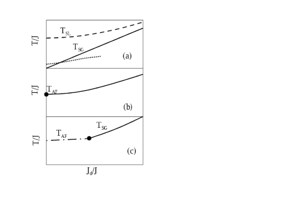
Figure 1: Schematic phase diagrams of the disordered AF quantum Heisenberg model in (a) $D=2$, (b) $D=3$, and (c) $D>4$. The dashed line $T_{SL}$ is a crossover temperature below which spin-liquid correlation appear. $T_{SG}$ and $T_{AF}$ are the spin-glass and the AF transition temperatures respectively. The dot schematically indicates the position at which the SG temperature becomes larger than the AF one. The dotted line indicates the “causal instability” line occurring in 2D (see text).

Fig. 1 schematically depicts the phase diagrams for our model in two, three, and above four dimensions. In two dimensions [Fig. 1(a)], the AF long-range order never occurs notemermin and AF correlations only manifest themselves with the formation of a spin-liquid phase with a reduced spin susceptibility (with respect to the Curie form valid at temperatures above $J$) and with critical spin dynamics. This behavior arises below a crossover temperature $T_{SL}$, which has been numerically determined via the QMC analysis reported in Section V. This will also allow for the quantitative determination of the SG transition temperature $T_{SG}$ and of the spin-liquid instability temperature $T^{*}$. This latter marks the temperature below which the spin self-energy $\Pi_{0}^{-1}(\omega)$ as a function of real frequencies has a positive imaginary part $\Pi_{0}^{-1}(\omega)^{\prime\prime}>0$ thereby violating the causality condition $\omega\Pi_{0}^{-1}(\omega)^{\prime\prime}<0$. BGG ; haule

In three dimensions Fig. 1(b) shows that, as soon as a disordered three-dimensional magnetic coupling $J_{D}$ is turned on, the system undergoes a second-order transition to a SG state. This occurs below a transition temperature $T_{SG}$, which, according to our criterion above, is always larger than the Néel temperature $T_{N}$ (in particular it is also larger than the AF temperature in the absence of disorder $T_{N}^{0}$. In the opposite limit of $J_{D}\gg J$ one naturally recovers the transition temperature for the “pure” quantum Sherrington-Kirkpatrick model bray ; goldschmidt ; daniel-marcelo and the $T_{SG}/J$ curve smoothly approaches the straight line $T_{SG}=0.142J_{D}$.

We finally notice that the qualitative picture reported in Fig. 1(c) for the case above four dimensions, is in qualitative agreement with the mean-field calculations of Refs. FMSG, , where the competition between a SG and a ferromagnetic phase was studied.

IV Static properties

IV.1 The three-dimensional case

When the AF coupling is assumed to act in three dimensions, the spin-wave spectral density $\rho(\epsilon)$ takes a semielliptic form

$$\rho_{3D}(\epsilon)=\frac{2}{\pi J^{2}}\sqrt{J^{2}-\epsilon^{2}}~{}.$$ (24)

In this case the integral in Eq. (17) can be analytically performed to show that this equation is identically satisfied for

$$\Pi_{0}^{-1}(\omega_{n})=J_{\times}^{2}\chi_{loc}(\omega_{n})~{},$$ (25)

with

$$J_{\times}^{2}\equiv J^{2}/4+J_{D}^{2}.$$ (26)

Therefore in three dimensions the problem with mixed AF and disordered coupling becomes formally equivalent to a model with a rescaled coupling $J_{\times}$ only note3D .

IV.1.1 Phase diagram

Starting from the free-spin high-temperature regime, upon decreasing $T$, the magnetic correlations start to reduce the magnetic susceptibility. We therefore introduce a crossover temperature $T_{\times}$, which is arbitrarily defined as the temperature at which the local magnetic susceptibility is reduced by ten per cent with respect to the free moment Curie law $4T_{\times}\chi_{loc}(T_{\times})=0.9$. From the numerical calculations, we find $T_{\times}\approx 0.75J_{\times}$. Since we decided to use the AF magnetic coupling $J$ as the energy unit, we recast this relation as

$$\frac{T_{\times}}{J}\approx 0.75\sqrt{\frac{1}{4}+\left(\frac{J_{D}}{J}\right)^{2}}~{},$$ (27)

where the disordered part of the magnetic interaction is made explicit.

IV.1.2 Spin-glass temperature

Using the three-dimensional density of states Eq. (24), the SG criterion Eq. (LABEL:SGcondition) is

$$1=\frac{2}{\pi}\frac{J_{D}^{2}}{J^{2}}\int_{-J}^{J}\frac{\sqrt{1-\epsilon^{2}}}{\left[{\Pi_{0}^{-1}(\omega=0,T_{SG})+\epsilon}\right]^{2}}d\epsilon~{}.$$ (28)

Using the relation

$$\int_{-1}^{1}\frac{\sqrt{1-x^{2}}}{\left[{y+x}\right]^{2}}dx=\frac{\pi}{\sqrt{y^{2}-1}}\left[{y-\sqrt{y^{2}-1}}\right]~{},$$ (29)

the SG criterion can be written as

$$\sqrt{\left({\frac{\Pi_{0}^{-1}}{J}}\right)^{2}-1}=2\frac{J_{D}^{2}}{J^{2}}\left[{\frac{\Pi_{0}^{-1}}{J}-\sqrt{\left({\frac{\Pi_{0}^{-1}}{J}}\right)^{2}-1}}\right]~{}.$$ (30)

Finally, this criterion can be cast into the form

$$\left|{\frac{\Pi_{0}^{-1}}{J}}\right|=\frac{1+2(J_{D}/J)^{2}}{\sqrt{1+4(J_{D}/J)^{2}}}~{}.$$ (31)

It is worth emphasizing again that the self-consistent value of $\Pi_{0}^{-1}(T_{SG})$ to be used in the above relations is the same as in the non-disordered system. Therefore, to determine the 3D phase diagram as a function of temperature and disordered coupling $J_{D}$, we self-consistently calculated with QMC the spin self-energy at different temperatures for a unit value of $J_{\times}=J=1$. The results are reported in the inset of Fig. 2. Then, for each value of $J_{D}/J$, the SG instability temperature is obtained by equating $\Pi_{0}^{-1}(T=T_{SG})$ with the r.h.s. of Eq.(31). While Fig. 1 is a sketch comparing the phase diagrams of our model in various dimensions, Fig. 2 shows the phase diagram in three dimensions as numerically determined from the procedure outlined above.

It is worth noticing that in the three-dimensional case the regime with strong spin correlations reducing the local susceptibility is severely reduced by the occurrence of the SG phase. This is to be contrasted with the substantial spin-liquid regime found in two dimensions (see next Section)

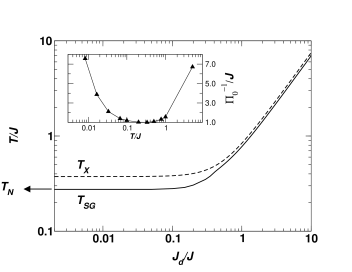
Figure 2: Phase diagram of the DQAFH model in three dimensions as obtained from the QMC calculations at fixed (unit) value of ${J_{\times}}$. The solid line represents the SG transition temperature $T_{SG}$ as numerically obtained from the criterium of Eqs. (LABEL:SGcondition) and Eq. (31). The dashed line is the crossover $T_{\times}$ (see text). Inset: zero-disorder spin self-energy $\Pi_{0}^{-1}$ as a function of temperature. The antiferromagnetic instability occurs at $T\approx 0.28J$, when $\Pi_{0}^{-1}=J$.

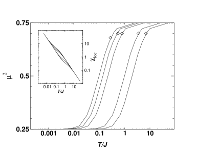
Figure 3: Temperature dependence of the square effective moment $\mu^{2}(T)=T\chi_{loc}(T)$ in 3D at fixed (unit) value of $J_{\times}$ and various values of disorder: $J_{D}/J=0,\,0.5,\,1.,\,5,\,10$ from left to right. The high-temperature limiting value is $S(S+1)=3/4$, while the low-temperature limit is $1/4$. The diamonds show the square moment at the corresponding $T_{SG}$. Inset: Temperature dependence of the local spin susceptibility for $J_{D}/J=0,\,0.5,\,1,\,5,\,10$ from top to bottom.

IV.1.3 Local-moment formation

The temperature dependence of the static local susceptibility is shown in the inset of Fig. 3 for various values of the disorder $J_{D}/J$ at a fixed value of $J_{\times}$. Again, by exploiting the fact that in the three-dimensional case the disordered coupling can be “hidden” inside the effective coupling $J_{\times}$, we first worked in units of $J_{\times}$, and calculated once the universal curve $J_{\times}\chi_{loc}(T,J_{D},J)=f(T/J_{\times})$). Then we expressed $J_{\times}$ in terms of $J_{D}/J$ to find the different curves at various values of disorder in the (meta)stable paramagnetic region, both above and below $T_{SG}$. It is quite evident that the susceptibility curves display both a high-temperature and a low-temperature Curie-like behavior with a constant (unity in log-log plot) universal slope. This is an indication of local moment formation, as shown in the main frame of Fig. 3. Here the temperature dependence of the square local moments $\mu^{2}(T)=T\chi_{loc}(T)$ is displayed, showing that $\mu(T)^{2}\approx 3/4$ at high temperature, while $\mu(T)^{2}\approx 1/4$ at low temperature. It can also be noticed that the disordered coupling strongly favors the formation of static low-T local moments. However, as shown by the diamonds in Fig. 3, the SG transition already occurs at much higher temperatures when the local moments are still close to their high-temperature value $3/4$.

IV.2 The two-dimensional case

We also consider here the case of two-dimensional AF fluctuations having a spectral density of the form $\rho_{2D}(\epsilon)=\frac{1}{2J}$ for $-J\leq\epsilon\leq J$. Contrary to the above 3D case, the effect of disorder can no longer be included in an effective coupling $J_{\times}$ together with the AF $J$. Therefore, for any value of $J_{D}$ one has to recalculate the self-consistent quantities $\chi_{loc},\,\,{\cal K}$. These quantities are related by the selfconsistency Eq.(17), which in two dimensions, reads

$$\Pi_{0}^{-1}(\omega,T)=J\coth\left[J\chi_{loc}(\omega,T)\right]~{}.$$ (32)

IV.2.1 Phase diagram

The results of our EDMFT calculations are summarized in the numerical phase diagram of Fig. 5.

Figure 4: Phase diagram of the DQAFH model in two dimensions as obtained from the QMC calculations. The dashed line represents the analytic estimation of the crossover temperature $T_{\times}$ the high-temperature free-spin regime to the intermediate-temperature spin-liquid regime as obtained from the high-temperature expansion (see text). The filled diamonds represent the SG transition temperature $T_{SG}$ as numerically obtained from the criterium of Eq. (LABEL:SGcondition). The heavy dashed line represents the asymptotic ($J_{D}\gg J$ transition line for the quantum Sherrington-Kirkpatrick model. The dot-dashed line corresponds to the temperature $T^{*}$ of the causality violation occurring at zero disorder, while the thin solid line is obtained from the low-temperature estimation of $T_{SG}$.

Here the presence of various regions is apparent, where the system displays different physical properties. First of all one should notice a crossover line separating the free-spin high temperature region from a region at intermediate temperatures and low disorder, where the spin system has non-trivial correlations. This crossover temperature has been determined from a high-temperature expansion of Eq. (32), where the explicit form of $\Pi_{0}^{-1}$ in 2D has been inserted. Specifically, by assuming that $J\chi_{loc}$ is small at high temperatures, one obtains that

$$\frac{T_{\times}}{J}=A\sqrt{1+9\left({\frac{J_{D}}{J}}\right)^{2}}~{}.$$ (33)

The prefactor $A$ is then numerically determined, by imposing that the spin susceptibility is reduced by ten percent from its high-energy Curie law. This yields $A\approx 0.25$, for which one obtains the dashed line in Fig. 4. Below this line and before the SG phase takes place at low temperature, the spins form a correlated “liquid” with the static and dynamic local susceptibilities showing anomalous power-law behavior. This behavior, at intermediate temperatures where the effects of $J_{D}$ are not significant, is quite similar to the case of the pure two-dimensional system described in Ref. BGG, . Specifically, one finds over an order of magnitude in T, where the static local spin susceptibility displays the quantum-critical power-law behavior $\chi_{loc}(T)\approx J^{-1}(J/T)^{2/3}$. Related critical dynamical properties are found in the same region (see below). However, upon lowering the temperature, the paramagnetic phase is characterized by the gradual formation of local moments, whose temperature dependence for various values of the disorder is reported in Fig. 5.

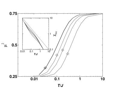
Figure 5: Temperature dependence of the square effective moment $\mu^{2}(T)=T\chi_{loc}(T)$ in 2D at various values of disorder: $J_{D}/J=0,\,0.10,\,0.58,\,0.98,\,2.06$ from left to right. The high-temperature limiting value is $S(S+1)=3/4$, while the low-temperature limit is $1/4$. The circle in the $J_{D}/J=0$ curve shows the square moment at $T=T^{*}\approx 0.03J$. The diamonds show the square moment at the corresponding $T_{SG}$. Inset: Temperature dependence of the local spin susceptibility for $J_{D}/J=0,\,0.58,\,0.98,\,2.06$ from top to bottom. The dashed line is a guide for the eyes corresponding to a power-law behavior with an exponent $2/3$ to illustrate the intermediate spin-liquid behavior.

IV.2.2 Local-moment formation

The fact that disorder favors the formation of local moments at progressively larger temperatures, is made apparent by the flattening of the curves to the classical value 1/4. It is worth noticing that the tendency to form a finite local moment at low temperature is also present in the absence of disorder ($J_{D}=0$). This tendency was also just visible in our previous workBGG , in our QMC calculations at $T=J/100$. However, it was impossible to confirm this numerical hint by well-converged QMC calculations at lower temperatures notenomomentum . On the other hand, the static moment formation becomes quite clear in the presence of disorder.

IV.2.3 Spin-glass temperature

So far we have discussed the properties of the paramagnetic phase disregarding the possible occurrence of a SG instability as determined by Eq. (LABEL:SGcondition). In the present two-dimensional case, the relation Eq. (LABEL:SGcondition) characterizing the SG temperature can be simplified to

$$\Pi_{0}^{-1}(\omega=0,T_{SG})=\sqrt{J_{D}^{2}+J^{2}}\equiv\hat{J}~{},$$ (34)

with $\Pi_{0}^{-1}(\omega,T)$ given by Eq. (32) In the weak disorder limit $J_{D}<<J$, we approximate $\chi_{loc}$ by its zero disorder expression $J\chi_{loc}(\omega=0,T<<J)\approx 0.338(J/T)^{2/3}$ (see Fig. 1(b) of Ref. BGG, ). This gives the asymptotic behavior in the limit $J_{D}/J\rightarrow 0$

$$T_{SG}\approx J\left[\frac{0.338}{\ln\frac{J}{J_{D}}}\right]^{3/2}~{},$$ (35)

showing that a significant $T_{SG}$ can be obtained even for a small disorder. The numerical data seem indeed to be smoothly extended to this low-disorder behavior (see Fig. 4).

V Dynamical properties

V.1 Dynamical properties in 3D

From our QMC analysis we also obtained dynamical quantities in imaginary time. Fig. 6 displays the imaginary-time dependence of the local spin susceptibility $\chi_{loc}(\tau)$ in the paramagnetic phase. notaplot Indeed, although the system rapidly passes from a paramagnetic high temperature phase to a low-temperature SG phase (see Fig. 2), we follow the paramagnetic phase down to low temperatures to allow a comparison with the two-dimensional case, where the critical SG temperature is much lower. In this way we can investigate the role of dimensionality in determining the spin dynamics.

Figure 6: Imaginary-time dependence of the local susceptibility in three dimensions at different values of the inverse temperature $\beta J_{\times}=1,\,3,\,5,\,10,\,30,\,60,\,120$.

In $\chi_{loc}(\tau)$ one can recognize the different temperature regimes found in the static quantities and explored in detail in the previous study of the purely disordered case in Ref. daniel-marcelo, . This is quite obvious since, as already discussed for the static properties, our system in three dimensions is equivalent to a purely disordered Heisenberg model with an effective magnetic coupling [see Eq.(25)]. This equivalence turns out to be quite important, since the dynamical analysis involves a delicate procedure of extracting real-frequency information from data obtained in imaginary time or frequencies. This is usually a difficult task, but it is greatly simplified by the knowledge of well-established limits at low and high temperatures for the dissipative part of the local response $\chi_{loc}(\omega)$. This allows the construction of an interpolating function that successfully matches the numerical QMC data. Specifically one finds a high-temperature regime, where the spin dynamic absorption produces a Gaussian quasi-elastic peak

$$\frac{\chi_{loc}^{\prime\prime}(\omega)}{\pi\omega} = \frac{\beta S(S+1)}{3}\left[1-S(S+1)\frac{(\beta{J_{\times}})^{2}}{18}\right]$$ (36)

$$\times \frac{e^{-1/2(\omega/\omega_{L})^{2}}}{\sqrt{2\pi\omega_{L}^{2}}}~{},$$

with a single characteristic relaxation frequency $\omega_{L}$ given by $\omega_{L}^{2}=2{J_{\times}}^{2}S(S+1)/2[1-S(S+1)(\beta{J_{\times}})^{2}/18]$ In imaginary-time this corresponds to

$$\chi_{loc}^{L}(\tau) = \frac{S(S+1)}{3}e^{-\frac{1}{2}\left(\frac{\beta\omega_{L}}{2}\right)^{2}\left[1-\left(1-\frac{2\tau}{\beta}\right)^{2}\right]}$$ (37)

$$\equiv \frac{S(S+1)}{3}\Phi_{L}(\tau)~{}.$$

On the other hand, at low temperatures the curves in Fig. 6 clearly display two regimes: At long times the curve flattens indicating the formation of nearly static moments, while at short times a rapid variation (decrease) of $\chi_{loc}(\tau)$ indicates that some spectral weight is shifted at high frequencies. From an analysis similar to the one of Ref. daniel-marcelo, one can see that this leads to dissipation from transverse spin excitations

$$\frac{\chi_{loc}^{T}(\omega)}{\pi\omega}=\frac{S}{2}\left[\frac{\beta}{2\omega_{T}}\right]^{3/2}\frac{\omega\tanh(\beta\omega/2)}{\sqrt{2\pi}(1+\beta\omega_{T}/2)}$$

$$\times \left[\exp\left[-\frac{\beta(\omega-\omega_{T})^{2}}{4\omega_{T}}\right]+\exp\left[-\frac{\beta(\omega+\omega_{T})^{2}}{4\omega_{T}}\right]\right]~{},$$

at frequencies $\omega_{T}\sim{J_{\times}}^{2}/T$. In imaginary time this gives

$$\chi_{loc}^{T}(\tau) = \frac{S(S+1)}{3}\frac{1+\beta\omega_{T}/2(1-2\tau/\beta)^{2}}{1+\beta\omega_{T}/2}$$ (39)

$$\times \exp\left[{-\frac{\beta\omega_{T}}{4}\left[1-\left(1-\frac{2\tau}{\beta}\right)^{2}\right]}\right]$$

$$\equiv \frac{S(S+1)}{3}\Phi_{T}(\tau)~{}.$$

The longitudinal fluctuations instead still produce a quasi-elastic absorption peak of the form of Eq. (36), but with a reduced frequency $\omega_{L}\propto T$ and a prefactor $\beta S^{2}/3$ replacing $\beta S(S+1)/3$. This reduction of the effective Curie constant is natural since the formation of static moments must coexist with the high-energy absorption.

The known behavior in the high- and low-temperature regimes allows to construct an interpolation function

$$\chi_{loc}=\frac{S(S+1)}{3}\left[p\Phi_{L}(\tau)+(1-p)\Phi_{T}(\tau)\right]~{}.$$ (40)

Obviously the temperature variation of the relaxation function $F(\omega)\equiv\chi^{\prime\prime}(\omega)/(\pi\chi_{loc}(T)\omega)$ is quite similar to the one shown in Fig. 2 of Ref. daniel-marcelo, provided that $J$ is replaced by ${J_{\times}}$.

V.2 Dynamical properties in 2D

Fig. 7 displays the results of our QMC calculations for the imaginary-time dependent spin susceptibility. The frames from top to bottom are for different values of disorder $J_{D}=0.1J$, $J_{D}=J$, and $J_{D}=10J$. The various curves are calculated at different values of the inverse temperature $\beta\hat{J}=1,\,3,\,5,\,10,\,30,\,60$. Frames (b) and (c) also contain the curves for $\beta\hat{J}=120$, which could not be obtained for the zero disorder case due to non-convergence of the QMC code. Similarly to the 3D case, the low-temperature curves clearly display a flattening at large time marking the tendency to form static local moments. This formation is clearly favored by disorder. The same conclusion could qualitatively be drawn from the local susceptibility as a function of Matsubara imaginary frequencies for various values of the disorder: At low temperature the more disordered systems display a visible tendency to form an additional contribution at zero frequency, which cannot be obtained from a smooth extrapolation from the finite-frequency data. This is because the local moments provide a substantial delta-like contribution to the zero-frequency susceptibility (however, due to the difficulty in reliably extracting this additional contribution, we refrain from showing curves for $\chi_{loc}(\omega_{n})$). For the curves of $\chi_{loc}$ as a function of imaginary-time, we performed an analysis similar to the one carried out in Subsection V.A for the three-dimensional case.

Upon inspecting the two-dimensional phase diagram of Fig. 4 one sees that a substantial region is present between $T_{\times}$ and $T^{*}$ or $T_{SG}$, where strong spin correlations should give rise to a non-trivial spin dynamics. From our previous work on the non-disordered Heisenberg model in two dimensions BGG , we learned that a spin-liquid phase arises below $T_{\times}$. At long imaginary times this phase has a critical susceptibility of the form $\chi_{loc}(\tau)\sim[sin(\pi\tau/\beta]^{-1/3}$, which corresponds to a scaling of the imaginary local susceptibility BGG

$$\chi^{\prime\prime}_{loc}(\omega)\sim J^{-1}(\omega/J)^{-\delta}{\cal F}_{\delta}(\omega/T)~{},$$ (41)

with ${\cal F}_{\delta}(x)=x^{\delta}|\Gamma(\frac{1-\delta}{2}+i\frac{x}{2\pi})|^{2}\sinh\left(\frac{x}{2}\right)$ and $\delta=2/3$. Eq. (41) gives a power-law divergence at low energy, $\chi^{\prime\prime}_{loc}(T=0,\omega)\sim J^{-\frac{1}{3}}\omega^{-\frac{2}{3}}$ and $\chi^{\prime}_{loc}(T,\omega=0)\sim J^{-\frac{1}{3}}T^{-\frac{2}{3}}$.

The question then naturally arises, whether or not this critical behavior can be experimentally observed in magnetic systems with strong quantum fluctuations, weak disorder, and strong anisotropy in the AF fluctuations.

In principle one could answer this question by extending the analysis of Subsect. V.A and generalizing Eq. (40) to a form including an additional spin-liquid contribution

$$\chi_{loc}=\frac{S(S+1)}{3}\left[p\Phi_{L}(\tau)+q\Phi_{SL}(\tau)(1-p-q)\Phi_{T}(\tau)\right]~{}.$$ (42)

with $\Phi_{SL}(\tau)\propto[sin(\pi\tau/\beta]^{-1/3}$. Starting from the Fourier transform of Eq. (42), we tried to use a standard procedure based on Padé approximants to analytically continue the Matsubara susceptibility to real frequencies. Unfortunately, the analytic continuation procedure is so delicate that reliable results can hardly be extracted from a form like Eq. (42). In particular we noticed that small variations in the relative weights $p,q$ as well as in the other physical parameters $\omega_{L}$ and $\omega_{T}$ lead to substantial variations in the real-frequency susceptibility. Therefore, while our analysis is fully compatible with the possibility of intermediate frequency windows with anomalous spin-liquid exponents, we cannot provide reliable bounds to the observation of these regimes.

Figure 7: Imaginary-time dependence of the local susceptibility in $D=2$ for different values of the inverse temperature $\beta\hat{J}=1,\,3,\,5,\,10,\,30,\,60,\,120$ and three values of disorder: (a) $J_{D}=0.1J$, (b) $J_{D}=J$, and (c) $J_{D}=10J$. For the low-disorder case (a) the lowest-temperature data $\beta\hat{J}=120$ are not available (see text).

VI Discussion and conclusions

In this paper we systematically investigated the interplay between disorder and fluctuations in a quantum spin-$\frac{1}{2}$ Heisenberg model. Without entering any broken-symmetry phase and neglecting the possible occurrence of first-order transitions, we investigated the properties and the instabilities of the paramagnetic phase. We found that a marked difference exists between the two- and the threedimensional cases. In 3D the system is ordered at a finite Néel temperature $T_{AF}$ for zero disorder and becomes a SG at $T_{SG}>T_{AF}$ as soon as a finite disorder is introduced in the magnetic coupling. This result is not so surprising because the AF and the SG phase are not competing so that antiferromagnetism can well coexist with glassiness at least for small disorder. According to these indications, in real AF systems the presence of a small amount of disorder is expected to lead to weak glassy properties. These, however, can likely be masked by the dominant (at weak disorder) AF properties.

The two-dimensional case is richer. In the absence of disorder, the spin liquid phase analyzed in Ref. BGG, was shown to be unstable below a temperature $T^{*}\sim 0.03J$, where the causality condition $\omega\Pi_{0}^{-1}(\omega)^{\prime\prime}<0$ on the self-energy of the dynamical local spin susceptibility starts to be violated. As discussed in detail in Ref. rosch, for the $t-J$ model, this behavior occurs when long ranged space correlations arise at finite temperature being driven by a divergent magnetic coherence length $\xi$. In this case in 2D the real part of the local susceptibility diverges because the momentum-independent spin self-energy introduced in the EDMFT approach is unable to produce anomalous dimensions (and the related $\eta$ exponent). Then $\chi_{loc}^{\prime}(0)\sim\log\xi$ (unphysically above the bare Curie value falk $S(S+1)/3T$). This growth at low (but still finite) temperatures entails too large values of the imaginary part of $\chi_{loc}^{\prime\prime}$, which give an unphysical sign of the spin self-energy determined by the self-consistency condition Eq. (32). This occurs at the “causal instability” temperature $T^{*}$. Nevertheless, the system may display an anomalous behavior of the spin susceptibility over broad frequency and temperature ranges before the instability occurs. Therefore the EDMFT treatment keeps a valuable physical interest to detect non-trivial spin correlations in low dimensions. Furthermore, we showed here that the causal instability may be prevented by a small amount of disorder: As seen in Fig. 4, already at $J_{D}\approx(0.05-0.1)J$ the SG transition temperature overcomes $T^{*}$. This also indicates that EDMFT acquires further interest and validity to treat those models where physical mechanisms prevent the large growth of the local susceptibility or induce the transition to a stable phasenotatstar .

A noticeable finding of this paper is also related to the specific form of the EDMFT kernel obtained in Eq. (13). In particular, as shown in Subsect. II.A and in Appendix B, the kernel separates into a AF and a disordered part (although disorder is effectively present in both terms via the averaged $\chi_{ij}$’s) and moreover the disordered kernel is build up with the local susceptibility only

$${\cal K}_{D}=(J_{D}/z)\sum_{i}{\overline{\chi}}_{ii}~{}.$$ (43)

The crucial ingredient leading to these two results were the local nature of the disorder ($\langle J_{ij}^{D}J_{kl}^{D}\rangle_{dis}=\delta_{i,l}\delta_{j,k}J_{D}^{2}$) and the large coordination of the lattice ($z\to\infty$). It is interesting to notice that the specific form in Eq.(43) of the disorder-kernel holds for any lattice type and is clearly reminiscent of the form obtained in the case of an ordered system on a Bethe latticereviewDMFT . Formally this arises because ${\cal K}_{D}$ is only non-vanishing for $\langle J_{ij}^{D}J_{kl}^{D}\rangle_{dis}=\delta_{i,l}\delta_{j,k}J_{D}^{2}$, which also holds in the specific case of the Bethe lattice where only fully retraceable paths are allowed. One consequence of the generic validity of Eq. (43) is that the results of Bray and Moore in Ref. bray, are naturally recovered here (both in two and three dimensions) in the limit of zero AF coupling. Indeed the (cubic) lattice with infinite-range interaction of Ref. bray, becomes equivalent to a lattice with infinite coordination because the role of the thermodynamic limit ($N\to\infty$, with $N$ number of sites) is replaced here by the $z\to\infty$ limit. Since the specific form of the lattice becomes immaterial for Gaussian (local) disorder, our results in the $J_{D}/J\to\infty$ limit where ${\cal K}\approx{\cal K}_{D}$ recover both the variational and the QMC results of Refs. bray, ; daniel-marcelo, . In particular, as shown in Sect.IV, we find the known linear dependence $T_{SG}=0.142J_{D}$ both in 2D and 3D. Our results, however, also show that in the presence of a uniform AF coupling the SG transition temperature occurs at values larger than the above linear behavior. Physically this occurs because quantum and thermal fluctuations are naturally decreased and severely suppressed by the occurrence of the AF phase in 3D. In other words, once AF correlations nearly quenches the spins, a (even small) disorder $J_{D}$ easily produces a glassy state at finite temperature $T_{SG}$ In 2D this mechanism is still present but weaker, because the AF order does not establish and the spin fluctuations are only reduced by the spin-liquid correlations. Then $T_{SG}$ vanishes for $J_{D}$ tending to zero, but slowly because of the logarithmic dependence in Eq. (35).

Appendix A Derivation of the local action

A.1 The replica trick

We consider the DQAFH model defined by the Hamiltonian Eq. (1), and we consider the effect of disorder within the replica trickReplicatrick . The replica trick relies on the assumption that the free energy ${\cal F}$ of the system is a self-averaging quantity. This means that in the thermodynamic limit the free energy does not depend on the configuration chosen for the random couplings $J_{ij}^{D}$. As a consequence, ${\cal F}$ remains unchanged when it is averaged with respect to all the possible configurations of $J_{ij}^{D}$, and we find

$$\beta{\cal F} = \langle log{\cal Z}(J_{ij}^{D}\rangle_{dis}$$ (44)

$$= \lim_{n\rightarrow 0}\frac{\langle{\cal Z}(J_{ij}^{D})\rangle_{dis}-1}{n}$$

$$= \lim_{n\rightarrow 0}\frac{1}{n}log\langle{\cal Z}^{n}(J_{ij}^{D})\rangle_{dis}~{},$$

where ${\cal Z}(J_{ij}^{D})$ is the partition function of the system for a given configuration of $J_{ij}^{D}$, and $\langle\cdots\rangle_{dis}$ denotes an average with respect to the probability distribution $P(J_{ij}^{D})$.

One of the replica trick hypotheses consists of assuming that the average $\langle{\cal Z}^{n}(J_{ij}^{D})\rangle_{dis}$ is an analytical function of $n$. We can thus express this quantity for integer values of $n$, interpreting ${\cal Z}^{n}(J_{ij}^{D})$ as being the partition function of $n$ replicas of the system which are independent of each other but characterized by the same distribution of $J_{ij}^{D}$. This is formally expressed by the relation

$$\langle{\cal Z}^{n}(J_{ij}^{D})\rangle_{dis}=\prod_{i<j}\int_{-\infty}^{+\infty}dJ_{ij}^{D}P(J_{ij}^{D})Tr\left[\exp-\sum_{\alpha=1}^{n}H_{\alpha}\right]~{},$$ (45)

where $H_{\alpha}$ is the disordered Heisenberg Hamiltonian Eq. (1) acting on the replica $\alpha$. In Eq.(3), the trace $Tr$ is applied to all the operators ${\bf S}_{i}^{\alpha}$ of the replicated Hilbert space. Here, the integration with respect to $J_{ij}^{D}$ generates an effective action with the following properties:
(i) The corresponding effective model now recovers the translational symmetry of the underlying lattice. This allows a dynamical mean field (DMFT) approach.
(ii) The spins of the same replica are coupled through the antiferromagnetic exchange $J_{ij}^{AF}$, and an antiferromagnetic (AF) instability can occur.
(iii) Some correlations occur between different replicas of the same spin, which could give rise to a ground state characterized by a replica symmetry breaking. This state would describe a SG phase.

A.2 DMFT and the local partition function

Following the usual DMFT approachreviewDMFT , we consider the local effective partition function seen from a given site of the lattice, that we arbitrarily denote $i=0$. As a preliminary, we introduce the ’cavity’ Hamiltonian $H^{(0)}$, corresponding to the Hamiltonian $H$ without the site $i=0$. The complete Hamiltonian is related to the cavity one with

$$H=H^{(0)}+\sum_{j\neq 0}V_{0j}~{},$$ (46)

with

$$V_{0j}=\frac{J_{0j}^{AF}+J_{0j}^{D}}{\sqrt{z}}\sum_{\alpha=1}^{n}{\bf S}_{0}^{\alpha}{\bf S}_{j}^{\alpha}~{},$$ (47)

describing the magnetic interaction between the site $i=0$ and its neighbors. The usual static mean field approximation consists of replacing this term by its average with respect to the thermal and disorder fluctuations. In a paramagnetic phase, this contribution would vanish and we would have to go beyond the static mean field, within the DMFT approach. Using a path integral formalism, the partition function of the replicated system is given by

$${\cal Z}^{n}(J_{ij}^{D})=Tr{\cal T}\exp\left[-\int_{0}^{\beta}d\tau H(\tau)\right]~{},$$ (48)

where ${\cal T}$ is the imaginary time ordering and the trace $Tr$ denotes a path integral, taken with respect to all the spin degrees of freedom ${\bf S}_{i}^{\alpha}(\tau)$. This is now formally performed in two steps $Tr=Tr_{0}Tr^{(0)}$, by considering first all the degrees of freedom concerning the sites $j\neq 0$ ($Tr^{(0)}$), and then computing the partial trace for the local spin operators on site $i=0$ ($Tr_{0}$). We find

$${\cal Z}^{n}(J_{ij}^{D}) =$$

$$Tr_{0}Tr^{(0)} {\cal T}\exp\left[-\int_{0}^{\beta}d\tau\left(H^{(0)}(\tau)-\sum_{j\neq 0}V_{0j}(\tau)\right)\right]~{}.$$

We average this relation with respect to the random distribution of the couplings $J_{ij}^{D}$, assuming that the probability distribution $P(J_{ij}^{D})$ has no correlation between two different pairs of sites $(i,j)$. The averages for the cavity (with $H^{(0)}$) and the local (with $V_{0j}$) parts can thus be factorized

$$\langle{\cal Z}^{n}(J_{ij}^{D})\rangle_{dis}={\cal Z}^{(0)}$$ (50)

$$\times \langle{Tr_{0}\langle{{\cal T}\exp\left[-\sum_{j\neq 0}\int_{0}^{\beta}d\tau V_{0j}(\tau)\right]}\rangle^{(0)}}\rangle_{dis}~{},$$

where

$${\cal Z}^{(0)}=\langle Tr^{(0)}{\cal T}\exp\left[-\int_{0}^{\beta}d\tau H^{(0)}(\tau)\right]\rangle_{dis}~{},$$ (51)

and $\langle\cdots\rangle^{(0)}$ denotes the thermal and disorder average with respect to the cavity Hamiltonian $H^{(0)}$. This is performed by using a cumulant expansion, using the general formula $\langle{\cal T}\exp[A]\rangle^{(0)}={\cal T}\exp[\sum_{p=1}^{+\infty}C_{p}/p!]$, where $A=-\sum_{j\neq 0}\int_{0}^{\beta}d\tau V_{0j}(\tau)$ and $C_{p}$ is the $p-$order cumulant, which invokes correlation functions between $p$ operators ${\bf S}_{j}^{\alpha}$. The usual static mean field approximation would consist of neglecting all the cumulants $p\geq 2$. But, since here we consider the paramagnetic phase, all the cumulants $C_{p}$ with odd $p$ vanish. Furthermore, in the limit $z\to\infty$ we find $C_{p}\approx z^{1-p/2}$, and $\langle{\cal T}\exp[A]\rangle^{(0)}={\cal T}\exp[C_{2}/2]$. The DMFT approach, which is exact in the limit of a large coordination number $z$, thus consists of approximating the relation Eq. (50) with

$$\langle{\cal Z}^{n}(J_{ij}^{D})\rangle_{dis}={\cal Z}^{(0)}\langle{Tr_{0}\langle{{\cal T}\exp{\frac{C_{2}}{2}}}\rangle^{(0)}}\rangle_{dis}~{},$$ (52)

where

$$C_{2}=\int_{0}^{\beta}d\tau\int_{0}^{\beta}d\tau^{\prime} \sum_{\nu\nu^{\prime}}\sum_{\alpha\alpha^{\prime}}S_{0\nu}^{\alpha}(\tau)S_{0\nu^{\prime}}^{\alpha^{\prime}}(\tau^{\prime})$$

$$\times \sum_{ij}\frac{J_{0i}J_{j0}}{z}\langle{{\cal T}S_{i\nu}^{\alpha}(\tau)S_{j\nu^{\prime}}^{\alpha^{\prime}}(\tau^{\prime})}\rangle^{(0)}~{}.$$

From this expression Eq. (4) is then obtained, which reduces to Eq. (14) in the paramagnetic case.

Appendix B Disorder average of the action kernel

B.1 Preliminaries

Our treatment of disorder proceeds along the following steps: First we fix the disorder configuration assuming a specific realization of the $J_{ij}^{D}$ distribution. Then, for this configuration one can closely follow the same steps as in Ref. smithsi, to derive the relation between the spin correlation functions with and without cavity

$$\chi_{ij}^{cavity}=\chi_{ij}-\chi_{i0}\chi_{0j}/\chi_{00}~{}.$$ (54)

Here, we want to establish a similar relation for the disorder-averaged susceptibilities $\overline{\chi}_{ij}$ defined by Eq. (9).

In general one can see that the various correlation functions are obtained by sums of the type

$${{\chi}}_{ij} = \delta_{ij}{\Pi}_{ii}-\frac{J_{ij}}{\sqrt{z}}{\Pi}_{ii}{\Pi}_{jj}$$

$$- \sum_{paths}\frac{(-1)^{p}J_{ii_{1}}J_{i_{1}i_{2}}\cdots J_{i_{p}j}}{z^{(p+1)/2}}{\Pi}_{ii}{\Pi}_{i_{1}i_{1}}\cdots{\Pi}_{i_{p}i_{p}}{\Pi}_{jj}~{},$$

where, to obtain the leading contribution in the large-$z$ expansion, the sum is taken over non-self-intersecting paths and the local correlations ${\Pi}$ take into account loop decorations of these paths. We will see in the following how these local propagators can be related to a local self-energy, which will be determined in a self-consistent way.

The relation (54) for the cavity susceptibility is obtained from Eq. (LABEL:Expansionchi) by using the general algebraic identity $\sum_{i\to 0}\sum_{0\to j}=[\sum_{i\to j}-\sum_{i\to j}^{cavity}]\sum_{0\to 0}$, where $\sum_{i\to j}$ represents a summation over all the direct paths between two sites $i$ and $j$, and $\sum_{i\to j}^{cavity}$ excludes all the direct paths through the site $0$.

B.2 Disorder averaging of the kernel

Here we will average the large$-z$ expansion (LABEL:Expansionchi) with respect to all the possible distributions of $J_{ij}^{D}$. First, we remark that a given bond $l-m$ (and the related $J_{lm}$) either appears in the product of $J$’s, forming the “skeleton” of the path, or is inside the loops forming one (and just one) of the $\Pi$’s. As a consequence, when taking the average over the disorder, each object, a $J$ or a ${\Pi}$ is separately averaged with respect to the others; therefore the average over the disorder distribution $P(J_{ij}^{D})$ factorizes in the average of each separate ${\Pi}$ and of the product of $J$’s. Furthermore one should notice that, since the paths are non-self-intersecting, the product of $J$’s can only contain one $J$ per $l-m$ bond. Therefore, owing to the zero average of the disordered $J^{D}$, this product vanishes unless it only contains purely AF ordered couplings. Then

$${\overline{\chi}}_{ij} = \delta_{ij}{\overline{\Pi}}_{ii}-\frac{J^{AF}_{ij}}{\sqrt{z}}{\overline{\Pi}}_{ii}{\overline{\Pi}}_{jj}$$

$$- \sum_{paths}\frac{(-1)^{p}J^{AF}_{ii_{1}}J^{AF}_{i_{1}i_{2}}\cdots J^{AF}_{i_{p}j}}{z^{(p+1)/2}}{\overline{\Pi}}_{ii}{\overline{\Pi}}_{i_{1}i_{1}}\cdots{\overline{\Pi}}_{i_{p}i_{p}}{\overline{\Pi}}_{jj}~{},$$

where the bar indicates disorder-averaged quantities. Then the same arguments used in Ref.  smithsi, for obtaining the relation (54) from the expansion (LABEL:Expansionchi), can now be applied to the averaged quantities of Eq. (LABEL:Expansionchiaverage) giving

$$\overline{\chi}_{ij}^{cavity}=\overline{\chi}_{ij}-\overline{\chi}_{i0}\overline{\chi}_{0j}/\overline{\chi}_{00}~{}.$$ (57)

This completes the derivation of Eq. (11) leading to the final expression of the kernel Eq. (13)

B.3 Local self-energy

The expansion (LABEL:Expansionchiaverage) is equivalent to a Bethe-Salpeter equation for the average susceptibilities

$${\overline{\chi}}_{ij}(\omega_{n})=\delta_{ij}{\Pi}_{0}(\omega_{n})-{\Pi}_{0}(\omega_{n})\sum_{l}\frac{J_{il}^{AF}}{\sqrt{z}}{\overline{\chi}}_{lj}(\omega_{n})~{},$$ (58)

where we restored the explicit Matsubara frequency dependency, and the averaged ${\Pi}_{0}\equiv\overline{\Pi}_{ii}$ is site independent.

Averaging the distribution of $J_{ij}^{D}$ restores the translational symmetry of the underlying lattice. We can thus define the ${\bf q}-$dependent susceptibilities $\chi({\bf q},\omega_{n})$ as the spatial Fourier transform of ${\overline{\chi}}_{ij}(\omega_{n})$. Introducing $J({\bf q})$, the Fourier transform of the magnetic exchanges $J_{ij}^{AF}/\sqrt{z}$, the Bethe-Salpeter Eq. (58) can be written as

$$\chi({\bf q},\omega_{n})=\left[{\Pi}_{0}^{-1}(\omega_{n})+J({\bf q})\right]^{-1}~{}.$$ (59)

The AF part ${\cal K}_{AF}$ of the Kernel is expressed in terms of the averaged susceptibilities using the definition [cf. Eq.(13)]

$${\cal K}_{AF}(\omega_{n}) = \frac{1}{z}\sum_{ij}J_{0i}^{AF}J_{j0}^{AF}\left[\overline{\chi}_{ij}(\omega_{n})\right.$$ (60)

$$\left.-\overline{\chi}_{i0}(\omega_{n})\overline{\chi}_{0j}(\omega_{n})/\overline{\chi}_{00}(\omega_{n})\right]~{}.$$

We rewrite this expression in momentum space:

$${\cal K}_{AF}(\omega_{n}) = \sum_{\bf q}J^{2}({\bf q})\chi({\bf q},\omega_{n})$$ (61)

$$- \left[\sum_{\bf q}J({\bf q})\chi({\bf q},\omega_{n})\right]^{2}/\chi_{loc}(\omega_{n})~{}.$$

Using this relation together with Eq. (59), and the identity $\chi_{loc}(\omega_{n})=\sum_{\bf q}\chi({\bf q},\omega_{n})$, we find

$$\Pi_{0}^{-1}(\omega_{n})={\cal K}_{AF}(\omega_{n})+\frac{1}{\chi_{loc}(\omega_{n})}~{}.$$ (62)

An explicit similar calculation can be found in Appendix C of Ref. smithsi,

References

- (1) * Deceased.
- (2) See, e.g., The Physics of Conventional and Unconventional Superconductors, edited by K.H. Bennemann and J.B. Ketterson, Springer Verlag, Berlin (2003).
- (3) G. R. Stewart, Rev. Mod. Phys. 73, 797 (2001); P. Coleman, Physica B 259-261, 353 (1999).
- (4) H. Weber and M. Vojta, cond-mat/0606753 and references therein.
- (5) J. Brooke, D. Bitko, T. F. Rosenbaum, and G. Aeppli, Science 284, 779 (1999).
- (6) We here adopt the term “spin-liquid” to indicate a magnetically correlated state, where low dimensionality, spin frustration, and/or quantum fluctuations prevent spin long-range order. In this state spin correlations reduce the Curie susceptibility to a much weaker power-low (or even logarithmic, see, Ref. sachdevye, ) behavior, and the spin fluctuations acquire critical dynamics with unusual weight at low frequencies.
- (7) S. Sachdev and J. Ye, Phys. Rev. Lett. 70, 3339 (1993).
- (8) C. Mondelli, H. Mutka, C. Payen, B. Frick, and K. H. Andersen, Physica (Amsterdam) 248 B, 1371 (2000).
- (9) A. Georges, O. Parcollet, and S. Sachdev, Phys. Rev. Lett. 85, 840 (2000).
- (10) A. Camjayi and M. J. Rozenberg, Phys. Rev. Lett. 90, 217202 (2003).
- (11) D. R. Grempel and M.J. Rozenberg, Phys. Rev. Lett. 80, 389, (1998).
- (12) J. L. Smith and Q. Si, Phys. Rev. B 61. 5184 (2000).
- (13) R. Chitra and G. Kotliar, Phys. Rev. Lett. 84, 3678 (2000).
- (14) S. Burdin, M. Grilli, and D. Grempel, Phys. Rev. B 67, 121104R (2003).
- (15) A. Georges et al., Rev. Mod. Phys. 68, 13 (1996).
- (16) K. Haule, A. Rosch, J. Kroha, and P. Wölfle, Phys. Rev. B 68, 155119 (2003).
- (17) S. Pankov, G. Kotliar, and Y. Motome, Phys. Rev. B 66, 045117 (2002).
- (18) M. Mezard, G. Parisi, and M. Virasoro, Spin glass theory and beyond, World Scientific Lecture Notes in Physics Vol.9, World Scientific.
- (19) S. Burdin, D. R. Grempel, and A. Georges, Phys. Rev. B 66, 045111 (2002).
- (20) Since (as usual is the Manhattan distance between sites and ) the second term if both and are nearest neighbors of site , [as they have to be in Eq. (13)]. Then, when the summation can be extended to independent and sites, a factor appears compensating the dependencies. This is not the case for the second term of the kernel when the disorder interaction is considered, since in this case there is the additional constraint , and only the part of the kernel survives.
- (21) J. L. Smith and Q. Si, Europhys. Lett. 45, 228 (1999).
- (22) A. M. Sengupta, Phys. Rev. B 61, 4041 (2000) and references therein.
- (23) Q. Si et al., Nature 413, 804 (2001).
- (24) A. J. Bray and M. A. Moore, J. Phys. C:Solid State Phys. 13, L655 (1980).
- (25) Formally the local model with pure disordered coupling is obtained taking the (implying ) in Eq. (LABEL:SGcondition).
- (26) The occurrence of a first-order transition near a quantum critical point was previously found in a quantum p-spin model [L. F. Cugliandolo, D. R. Grempel, and C. A. da Silva Santos, Phys. Rev. Lett. 85 2589 (2000)].
- (27) It is worth noticing that this result is reminiscent of the Harris criterion harris establishing the relevance of disorder on the critical behavior of systems with . Within the EDMFT approach leading to . However, the two criteria are physically distinct. While the Harris criterion arises from arguments based on fluctuations of the defect distribution on volumes of the order of the correlation length , our argument, which is specific to the EDMFT approach, does not apparently involve any relation between space fluctuations of and . This different physical content is also visible in the fact that our criterion does not involve the exponent . Indeed, one can introduce a “mass” term in the denominator of the integrand in (LABEL:SGcondition). However, for the integral diverges [as ] for any value of , thereby validating our criterion irrespectively from .
- (28) A. B. Harris, J. Phys. C:Solid State Phys. 7, 1671 (1974).
- (29) Notice that this is a consequence of the EDMFT formalism and, although compatible with, it is not a consequence of the Mermin-Wagner theorem. Indeed the same absence of an AF order at any finite T would still hold for an Ising model.
- (30) Y. Y. Goldschmidt and P. Y. Lai, Physica 177A, 544 (1991).
- (31) J. Villain, Z. Phys. B 33, 31 (1979); M. Gabay and G. Toulouse, Phys. Rev. Lett. 47, 201 (1981) and references therein.
- (32) Notice also that at this stage the self-consistent expression of the spin self-energy, as well as the related quantities and do not depend on disorder and have the same form of a 3D purely AF system. The only role of disorder in the paramagnetic phase we consider is to allow the application of the SG instability criterium Eqs. (LABEL:SGcondition).
- (33) Notice that in our previous work we also carried out analytic calculations within a large-N expansion. Obviously, since the large-N analysis is “by construction” unable to account for local moment formation, this occurrence was not considered in that framework.
- (34) To allow a comparison of the curves at different temperatures we plot the curves as functions of . Due to the bosonic character of the spin excitations, the curves are obviously periodic with period one in the variable.
- (35) This peculiar instability has also recently been found within an EDMFT treatment of the t-J model haule .
- (36) H. Falk and L. W. Bruch, Phys. Rev. 180, 442 (1969).
- (37) Recently we were able to push our QMC analysis to lower temperatures in the absence of disorder. We found that also in this case there are hints of the system having a tendency to form static local moments. In particular one can see in Fig. 5 that even the curve for displays a change of slope at low . This is further evidence that the spin system would like to enter an ordered phase (which is not allowed by our approach) and shifts spectral weight to larger frequencies. This shift, however, is not sufficient to control the exceeding increase of at low frequencies and does not prevent the causality catastrophe. Nevertheless it is useful to notice that any, even weak, additional physical mechanism leading to a further reduction of might help in avoiding the causality violation. Example in this sense are given by disorder, geometric frustration, which may prevent the tendency to magnetic ordering in favor of short-range singlet correlations.
- (38) If the sites were common to more than one loop decoration, the whole path consisting of “skeleton” and loops would go along a more constrained set of sites and would be of higher order in . In other words, in the limit of infinite coordination it is “very unlikely” that loop paths starting from different sites intersect.