Sum Rules for the Optical and Hall Conductivity in Graphene

Abstract

Graphene has two atoms per unit cell with quasiparticles exhibiting the Dirac-like behavior. These properties lead to interband in addition to intraband optical transitions and modify the $f$-sum rule on the longitudinal conductivity. The expected dependence of the corresponding spectral weight on the applied gate voltage $V_{g}$ in a field effect graphene transistor is $\sim\mbox{const}-|V_{g}|^{3/2}$. For $V_{g}=0$, its temperature dependence is $T^{3}$ rather than the usual $T^{2}$. For the Hall conductivity, the corresponding spectral weight is determined by the Hall frequency $\omega_{H}$ which is linear in the carrier imbalance density $\rho$, and hence proportional to $V_{g}$, and is different from the cyclotron frequency for Dirac quasiparticles.

I Introduction

The real part of frequency dependent optical conductivity $\sigma_{xx}(\Omega)$ is its absorptive part and its spectral weight distribution as a function of energy ($\hbar\Omega$) is encoded with information on the nature of the possible electronic transitions resulting from the absorption of a photon. Even though the relationship of the conductivity to the electronic structure and transport lifetimes is not straightforward, much valuable information can be obtained from such data. In particular, the $f$-sum rule on the real part of $\sigma_{xx}(\Omega)$ stated in its simplest form for an infinite free electron band,

$$\int_{0}^{\infty}d\Omega\mbox{Re}\sigma_{xx}(\Omega)=\frac{\omega_{P}^{2}}{8}$$ (1)

has proved particularly useful. Here $\omega_{P}$ is the plasma frequency, $\omega_{P}^{2}=4\pi ne^{2}/m$, with $n$ the free carrier density per unit volume, $-e<0$ the charge of electron, and $m$ its effective mass. In this case the right hand side (RHS) of Eq. (1) is independent of temperature and of the interactions. More generally for a finite tight binding band, the optical sum rule takes the form

$$\frac{2}{\pi}\int_{0}^{\Omega_{M}}d\Omega\mbox{Re}\,\sigma_{xx}(\Omega)=\frac{e^{2}}{\hbar^{2}V}\sum_{\mathbf{k},\sigma}n_{\mathbf{k},\sigma}\frac{\partial^{2}\epsilon_{\mathbf{k}}}{\partial k_{x}^{2}},$$ (2)

with $\Omega_{M}$ a cutoff energy on the band of interest and only the contribution to $\mbox{Re}\,\sigma_{xx}(\Omega)$ of this particular band is to be included in the integral. Here $\hbar$ is Planck’s constant, $V$ is the crystal volume, $\sigma$ is the spin, $\epsilon_{\mathbf{k}}$ is the electronic dispersion, $\mathbf{k}$ is the wave vector in the Brillouin zone, and $n_{\mathbf{k},\sigma}$ is the probability of occupation of the state $|\mathbf{k},\sigma\rangle$. If we assume a free electron dispersion, $\epsilon_{\mathbf{k}}=\hbar^{2}\mathbf{k}^{2}/2m$, Eq. (2) immediately reduces to Eq. (1) with $n=N/V$, where $N=\sum_{\mathbf{k},\sigma}n_{\mathbf{k},\sigma}$ is the total number of electrons in the band. For tight-binding dispersion with nearest neighbor hopping on a square lattice it is easy to show that the RHS of Eq. (2) reduces to $e^{2}/\hbar^{2}$ multiplied by minus one-half of the kinetic energy, $W_{\mathrm{K.E.}}$ per atom. In this particular case the optical sum rule can be used to probe the change in kinetic energy of the electrons as a function of temperature or with opening of a gap in the spectrum of the quasiparticle excitations which has been a topic of much recent research Hirsch1992PC ; Millis:book ; Marel:book ; Benfatto:review ; Carbotte:review .

When a constant external magnetic field $\mathbf{B}$ is applied to a metallic system in the $z$-direction, the optical conductivity acquires a transverse component $\sigma_{xy}(\Omega)$ in addition to the longitudinal component $\sigma_{xx}(\Omega)$. This quantity gives additional information on the electronic properties modified by the magnetic field. In this case Drew and Coleman Drew1997PRL have derived a new sum rule on the optical Hall angle $\theta_{H}(\Omega)$. If we define

$$t_{H}(\Omega)\equiv\tan\theta_{H}(\Omega)=\frac{\sigma_{xy}(\Omega)}{\sigma_{xx}(\Omega)},$$ (3)

then

$$\frac{2}{\pi}\int_{0}^{\infty}d\Omega\mathrm{Re}t_{H}(\Omega)=\omega_{H},$$ (4)

where $\omega_{H}$ is the Hall frequency which corresponds to the cyclotron frequency $\omega_{c}=eB/mc$ for free electrons. Here $c$ is the velocity of light.

Recently, graphene which is a single atomic layer of graphite, has been isolated Novoselov2004Science and studied Geim2005Nature ; Kim2005Nature (see Refs. rev1, ; rev2, for a review). The two-dimensional (2D) graphene honeycomb lattice has two atoms per unit cell. Its tight binding band structure consists of the conduction and valence $\pi$ bands. These two bands touch each other and cross the Fermi level, corresponding to zero chemical potential $\mu$, in six $\mathbf{K}$ points located at the corners of the hexagonal 2D Brillouin zone, but only two of them are inequivalent. The extended rhombic Brillouin zone can be chosen to contain only these two points inside the zone. In a field effect graphene device Novoselov2004Science ; Geim2005Nature ; Kim2005Nature electrons can be introduced in the empty conduction band or holes in the filled valence band through the application of a gate voltage and thus the normally zero value of the chemical potential $\mu$ can be changed continuously. In this paper we wish to consider the optical sum rules described above for the specific case of graphene. Two essential modifications arise. The existence of the two bands means that interband transitions need to be accounted for in addition to the usual intraband transitions of the previous discussion. Second, the electronic dispersion curves near $\mathbf{K}$ points are linear in momentum and the low-energy quasiparticle excitations are described by the “relativistic” $(2+1)$ dimensional Dirac theory Wallace1947PRev ; Semenoff1984PRL ; DiVincenzo1984PRB ; Gonzales1993NP rather than the Schrödinger equation.

The effective low-energy Dirac description of graphene turns out to be insufficient for the derivation of the sum rules. This can be easily understood from two examples. The RHS of Eq. (2) is normally related (Refs. Millis:book, ; Marel:book, ; Benfatto:review, ; Carbotte:review, ) to the diamagnetic term that is defined as the second derivative of the Hamiltonian [see Eq. (12) below] with respect to the vector potential. This term is zero within the Dirac approximation. On the other hand, it follows from the same Dirac approximation that, in the high-frequency limit, the interband contribution to conductivity is constant Gusynin2006micro ; Gusynin2007JPCM (see also Ref. Falkovsky2006, )

$$\mbox{Re}\sigma_{xx}(\Omega)\simeq\frac{\pi e^{2}}{2h},\qquad\Omega\gg\mu,T.$$ (5)

The frequency $\Omega$ is unbound in the Dirac approximation, although physically $\Omega$ should be well below the band edge. This example indicates that when considering sum rules one should go beyond the Dirac approximation.

The second example is that the cyclotron frequency $\omega_{c}$ for the Dirac quasiparticles Zheng2002PRB is defined in a different way, $\omega_{c}=eBv^{2}_{F}/(c|\mu|)$, where $v_{F}$ is the Fermi velocity. This definition follows from the fact that a fictitious relativistic mass Geim2005Nature ; Kim2005Nature ; Gusynin2006PRB $m_{c}=|\mu|/v_{F}^{2}$ plays the role of the cyclotron mass in the temperature factor of the Lifshits-Kosevich formula for graphene Sharapov2004PRB ; Gusynin2005PRB . This cyclotron frequency diverges as $\mu\to 0$, also posing the question as what one should use as a Hall frequency on the RHS of Eq. (4).

It turns out that these problems are resolved when a tight-binding model is considered, but still due to the specifics of graphene, the $f$-sum rule cannot be guessed from Eq. (2) applied for the two-band case. Further important modifications to the $f$-sum and Hall angle sum rule for graphene are expected and found in this paper.

The paper is organized as follows. In Sec. II we introduce the tight-binding model and the necessary formalism. In Secs. III and IV we describe the derivation of the sum rules for the diagonal and Hall conductivities and consider the specific case of graphene. The partial sum rule for the Hall angle is investigated in Sec. V. In Sec. VI, the main results of the paper are summarized. Mathematical details are given in two Appendices.

II Tight-binding model and general representation for electrical conductivity

II.1 Tight-binding model: Paramagnetic and diamagnetic parts

The honeycomb lattice can be described in terms of two triangular sublattices, A and B. The unit vectors of the underlying triangular sublattice are chosen to be

$$\begin{split}&\mathbf{a}_{1}=(a\sqrt{3}/2,a/2),\\ &\mathbf{a}_{2}=(a\sqrt{3}/2,-a/2),\end{split}$$ (6)

where the lattice constant $a=|\mathbf{a}_{1}|=|\mathbf{a}_{2}|=\sqrt{3}a_{CC}$ and $a_{CC}$ is the distance between two nearest carbon atoms. Any $A$ atom at the position $\mathbf{n}=\mathbf{a}_{1}n_{1}+\mathbf{a}_{2}n_{2}$, where $n_{1},n_{2}$ are integers, is connected to its nearest neighbors on $B$ sites by the three vectors $\boldsymbol{\delta}_{i}$:

$$\begin{split}&\boldsymbol{\delta}_{1}=-(\mathbf{a}_{1}+\mathbf{a}_{2})/3,\\ &\boldsymbol{\delta}_{2}=2/3\mathbf{a}_{1}-1/3\mathbf{a}_{2},\\ &\boldsymbol{\delta}_{3}=-1/3\mathbf{a}_{1}+2/3\mathbf{a}_{2}.\end{split}$$ (7)

We start with the simplest tight-binding description for $\pi$ orbitals of carbon in terms of the Hamiltonian

$$H=t\sum_{\mathbf{n},\boldsymbol{\delta},\sigma}\left[a_{\mathbf{n},\sigma}^{\dagger}\exp\left(\frac{ie}{\hbar c}\boldsymbol{\delta}\mathbf{A}\right)b_{\mathbf{n}+\boldsymbol{\delta},\sigma}+\mbox{c.c.}\right],$$ (8)

where $t$ is the hopping parameter, $a_{\mathbf{n},\sigma}$ and $b_{\mathbf{n}+\mathbf{\delta},\sigma}$ are the Fermi operators of electrons with spin $\sigma$ on $A$ and $B$ sublattices, respectively. Since we are interested in the current response, the vector potential $\mathbf{A}$ is introduced in the Hamiltonian (8) by means of the Peierls substitution $a_{\mathbf{n},\sigma}^{\dagger}b_{\mathbf{m},\sigma}\rightarrow a_{\mathbf{n},\sigma}^{\dagger}\exp\left(-\frac{ie}{\hbar c}\int_{\mathbf{m}}^{\mathbf{n}}{\bf A}d\mathbf{r}\right)b_{\mathbf{m},\sigma}$, which introduces the phase factor $\exp(\frac{ie}{\hbar c}\boldsymbol{\delta}\mathbf{A})$ in the hopping term (see Ref. Millis:book, for a review). We keep the Planck constant $\hbar$ and the velocity of light $c$, but set $k_{B}=1$.

Expanding the Hamiltonian (8) to the second order in the vector potential, one has

$$H=H_{0}-\sum_{\mathbf{n}}\left[\frac{1}{c}\mathbf{A}(\mathbf{n})\mathbf{j}(\mathbf{n})-\frac{1}{2c^{2}}A_{\alpha}(\mathbf{n})\tau_{\alpha\beta}(\mathbf{n})A_{\beta}(\mathbf{n})\right],\qquad\alpha,\beta=1,2.$$ (9)

The total current density operator is obtained by differentiating the last equation with respect to $A_{\alpha}(\mathbf{n})$,

$$j_{\alpha}(\mathbf{n})=-\frac{\partial H}{\partial\left(A_{\alpha}/c\right)}=j_{\alpha}^{P}(\mathbf{n})-\tau_{\alpha\beta}(\mathbf{n})A_{\beta}(\mathbf{n})/c,$$ (10)

and consists of the usual paramagnetic part

$$j_{\alpha}^{P}(\mathbf{n})=-\frac{ite}{\hbar}\sum_{\boldsymbol{\delta},\sigma}\delta_{\alpha}\left[a_{\mathbf{n},\sigma}^{\dagger}b_{\mathbf{n}+\boldsymbol{\delta},\sigma}-b_{\mathbf{n}+\boldsymbol{\delta},\sigma}^{\dagger}a_{\mathbf{n},\sigma}\right]$$ (11)

and diamagnetic part

$$\tau_{\alpha\beta}(\mathbf{n})=\frac{\partial^{2}H}{\partial\left(A_{\alpha}/c\right)\partial\left(A_{\beta}/c\right)}=-\frac{te^{2}}{\hbar^{2}}\sum_{\boldsymbol{\delta},\sigma}\delta_{\alpha}\delta_{\beta}\left[a_{\mathbf{n},\sigma}^{\dagger}b_{\mathbf{n}+\boldsymbol{\delta},\sigma}+b_{\mathbf{n}+\boldsymbol{\delta},\sigma}^{\dagger}a_{\mathbf{n},\sigma}\right].$$ (12)

II.2 Noninteracting Hamiltonian

The noninteracting Hamiltonian $H_{0}$ in Eq. (9) written in the momentum representation reads

$$H_{0}=\sum_{\sigma}\int_{BZ}\frac{d^{2}k}{(2\pi)^{2}}\Upsilon_{\sigma}^{\dagger}(\mathbf{k})\mathcal{H}_{0}\Upsilon_{\sigma}(\mathbf{k}),\qquad\mathcal{H}_{0}=\left(\begin{array}[]{cc}0&\epsilon(\mathbf{k})e^{i\varphi(\mathbf{k})}\\ \epsilon(\mathbf{k})e^{-i\varphi(\mathbf{k})}&0\\ \end{array}\right),$$ (13)

with $\phi(\mathbf{k})=t\sum_{\boldsymbol{\delta}}e^{i\mathbf{k}\boldsymbol{\delta}}\equiv\epsilon(\mathbf{k})e^{i\varphi(\mathbf{k})}$. The dispersion law $\epsilon(\mathbf{k})$ is

$$\epsilon(\mathbf{k})=t\sqrt{1+4\cos\frac{\sqrt{3}k_{x}a}{2}\cos\frac{k_{y}a}{2}+4\cos^{2}\frac{k_{y}a}{2}}.$$ (14)

In Eq. (13) we introduced the spinors

$$\Upsilon_{\sigma}(\mathbf{k})=\left(\begin{array}[]{c}a_{\sigma}(\mathbf{k})\\ b_{\sigma}(\mathbf{k})\\ \end{array}\right),$$ (15)

with the operator $\Upsilon_{\sigma}(\mathbf{k})$ being the Fourier transform of the spinor $\Upsilon_{\sigma}(\mathbf{n})=\left(\begin{array}[]{c}a_{\mathbf{n},\sigma}\\ b_{\mathbf{n},\sigma}\\ \end{array}\right)$:

$$\Upsilon_{\sigma}(\mathbf{n})=\sqrt{S}\int_{BZ}\frac{d^{2}{\mathbf{k}}}{(2\pi)^{2}}\,e^{i\mathbf{k}\mathbf{n}}\Upsilon_{\sigma}(\mathbf{k}).$$ (16)

Here $S=\sqrt{3}a^{2}/2$ is the area of a unit cell and the integration in Eqs. (13) and (16) goes over the extended rhombic Brillouin zone (BZ) which is characterized by the reciprocal lattice vectors $\mathbf{b}_{1}=2\pi/a(1/\sqrt{3},1)$ and $\mathbf{b}_{2}=2\pi/a(1/\sqrt{3},-1)$.

We also add the term

$$H_{0}\to H_{0}-\mu\sum_{\sigma}\int_{BZ}\frac{d^{2}k}{(2\pi)^{2}}\Upsilon_{\sigma}^{\dagger}(\mathbf{k})\hat{I}\Upsilon_{\sigma}(\mathbf{k})$$ (17)

with the chemical potential $\mu$ to the Hamiltonian $H_{0}$, so that our subsequent consideration is based on the grand canonical ensemble. The corresponding imaginary time Green’s function (GF) is defined as a thermal average

$$G_{\sigma}(\tau_{1}-\tau_{2},\mathbf{n}_{1}-\mathbf{n}_{2})=-\langle T_{\tau}\Upsilon_{\sigma}(\tau_{1},\mathbf{n}_{1})\Upsilon_{\sigma}^{\dagger}(\tau_{2},\mathbf{n}_{2})\rangle$$ (18)

and its Fourier transform is

$$G_{\sigma}(\tau_{1}-\tau_{2},\mathbf{n}_{1}-\mathbf{n}_{2})=T\sum_{n}\int_{BZ}\frac{d^{2}{\mathbf{k}}}{(2\pi)^{2}}G(i\omega_{n},\mathbf{k})\exp[-i\omega_{n}(\tau_{1}-\tau_{2})+i\mathbf{k}(\mathbf{n}_{1}-\mathbf{n}_{2})],$$ (19)

with

$$G(i\omega_{n},\mathbf{k})=\frac{(i\omega_{n}+\mu)\hat{I}+\sigma_{+}\phi(\mathbf{k})+\sigma_{-}\phi^{\ast}(\mathbf{k})}{(i\omega_{n}+\mu)^{2}-\epsilon^{2}(\mathbf{k})},\qquad\omega_{n}=\pi(2n+1)T,$$ (20)

where the matrix $\sigma_{\pm}=(\sigma_{1}\pm i\sigma_{2})/2$ made from Pauli matrices operates in the sublattice space. In Eq. (20) the spin label $\sigma$ is omitted, because in what follows we neglect the Zeeman splitting and include a factor of $2$ when necessary. The GF (20) describes the electronlike and holelike excitations with energies $E_{\pm}(\mathbf{k})=\pm\epsilon(\mathbf{k})-\mu$, respectively. The dispersion $\epsilon(\mathbf{k})$ near $\mathbf{K}$ points is linear, $E_{\pm}({\bf p})=\pm\hbar v_{F}\sqrt{p_{1}^{2}+p_{2}^{2}}-\mu$, where the wave vector ${\bf p}=(p_{1},p_{2})$ is now measured from the $\mathbf{K}$ points and the Fermi velocity is $v_{F}=\sqrt{3}ta/(2\hbar)$. Its experimental value Geim2005Nature ; Kim2005Nature is $v_{F}\approx 10^{6}\mbox{m/s}$.

II.3 Electrical conductivity

The frequency-dependent electrical conductivity tensor $\sigma_{\alpha\beta}(\Omega)$ is calculated using the Kubo formula Millis:book ; Marel:book

$$\sigma_{\alpha\beta}(\Omega)=\frac{K_{\alpha\beta}(\Omega+i0)}{-i(\Omega+i0)},\qquad K_{\alpha\beta}(\Omega+i0)\equiv\frac{\langle\tau_{\alpha\beta}\rangle}{V}+\frac{\Pi_{\alpha\beta}^{R}(\Omega+i0)}{\hbar V},$$ (21)

where the retarded correlation function for currents is given by

$$\Pi_{\alpha\beta}^{R}(\Omega)=\int_{-\infty}^{\infty}dt\,e^{i\Omega t}\Pi_{\alpha\beta}^{R}(t),\quad\Pi_{\alpha\beta}^{R}(t)=-i\theta(t){\rm Tr}\left(\hat{\rho}[J_{\alpha}(t),J_{\beta}(0)]\right),$$ (22)

$V$ is the volume of the system, $\hat{\rho}=\exp(-\beta H_{0})/Z$ is the density matrix of the grand canonical ensemble, $\beta=1/T$ is the inverse temperature, $Z={\rm Tr}\exp(-\beta H_{0})$ is the partition function, and $J_{\alpha}$ are the total paramagnetic current operators with

$$J_{\alpha}(t)=e^{iHt/\hbar}J_{\alpha}(0)e^{-iHt/\hbar},\qquad J_{\alpha}(t)=\sum_{\mathbf{n}}j_{\alpha}^{P}(t,\mathbf{n}),$$ (23)

expressed via the paramagnetic current density (11). Using the representation for $\Pi_{\alpha\beta}(\Omega)$ in terms of the matrix elements of the current operator $J_{\alpha}(t=0)$, one can find Shastry1993PRL the high-frequency, $\Omega\to\infty$ asymptotic of the Hall conductivity,

$$\sigma_{xy}(\Omega)=\frac{i}{V\hbar\Omega^{2}}\left\{\langle[J_{x},J_{y}]\rangle+\frac{1}{(\hbar\Omega)^{2}}\langle[[[J_{x},H],H]J_{y}]\rangle+O\left(\frac{1}{(\hbar\Omega)^{4}}\right)\right\},$$ (24)

while the longitudinal conductivity is

$$\sigma_{xx}=\frac{1}{iV\Omega}\left\{-\langle\tau_{xx}\rangle+\frac{1}{(\hbar\Omega)^{2}}\langle[[J_{x},H],J_{x}]\rangle+O\left(\frac{1}{(\hbar\Omega)^{4}}\right)\right\}.$$ (25)

Here $[,]$ is the commutator. Below in Secs. III and IV we will use Eqs. (21), (24), and (25) to outline the formal derivation of the sum rules.

III Diagonal optical conductivity sum rule

The optical conductivity sum rule is a consequence of gauge invariance and causality. Gauge invariance dictates the way that the vector potential enters Eq. (8) and, respectively, determines the diamagnetic and paramagnetic terms in the expansion (9) as well as the form of Kubo formula (21). The causality implies that the conductivity, Eq. (21) satisfies the Kramers-Krönig (KK) relation

$$\sigma_{\alpha\beta}(\Omega)=\frac{1}{\pi i}\mathrm{P}\int_{-\infty}^{\infty}\frac{d\omega\,\sigma_{\alpha\beta}(\omega)}{\omega-\Omega}.$$ (26)

Combining together the high-frequency limit of the KK relation (26),

$$\mathrm{Im}\sigma_{\alpha\beta}(\Omega)=\frac{1}{\pi\Omega}\mathrm{P}\int_{-\infty}^{\infty}d\omega\mathrm{Re}\sigma_{\alpha\beta}(\omega),\qquad\Omega\to\infty,$$ (27)

and the asymptotic (25), we arrive at the sum rule

$$\frac{1}{\pi}\int\limits_{-\infty}^{\infty}d\Omega\mathrm{Re}\sigma_{xx}(\Omega)=\frac{\langle\tau_{xx}\rangle}{V}.$$ (28)

Taking into account that $\mathrm{Re}\sigma_{xx}(\Omega)$ is an even function of $\Omega$, we observe that for a single tight-binding band $\langle\tau_{\alpha\beta}\rangle/V$ corresponds to the RHS of Eq. (2). Also defining the plasma frequency $\omega_{P}$ via $\omega_{P}^{2}/(4\pi)\delta_{\alpha\beta}\equiv\langle\tau_{\alpha\beta}\rangle/V$ we can rewrite the sum rule (28) in the form (1). Below we calculate this term for the Hamiltonian (8) with a nearest neighbor hopping on the hexagonal graphene lattice.

III.1 Explicit form of the diamagnetic term

The diamagnetic or stress tensor $\langle\tau_{\alpha\beta}\rangle$ in the Kubo formula (21) is a thermal average of Eq. (12)

$$\langle\tau_{\alpha\beta}\rangle=\langle\sum_{\mathbf{n}}\tau_{\alpha\beta}(\mathbf{n})\rangle.$$ (29)

This term is calculated in Appendix A and is given by

$$\frac{\langle\tau_{\alpha\alpha}\rangle}{V}=\frac{2e^{2}}{\hbar^{2}}\int_{BZ}\frac{d^{2}{\bf k}}{(2\pi)^{2}}\left[n_{F}\left(\epsilon(\mathbf{k})\right)-n_{F}(-\epsilon(\mathbf{k}))\right]\left[\frac{\partial^{2}}{\partial k_{\alpha}^{2}}-\left(\frac{\partial\varphi(\mathbf{k})}{\partial k_{\alpha}}\right)^{2}\right]\epsilon(\mathbf{k}),$$ (30)

where $n_{F}(\omega)=1/[\exp((\omega-\mu)/T)+1]$ is the Fermi distribution. Because the graphene structure contains two atoms per unit cell (two sublattices), there are two bands in the BZ which correspond to positive- and negative-energy Dirac cones. The momentum integration in Eq. (30) is over the entire BZ and the thermal factors $n_{F}(\epsilon(\mathbf{k}))$ and $n_{F}(-\epsilon(\mathbf{k}))$ refer to the upper and lower Dirac cones, respectively. We note that a simple generalization of Eq. (2) for a two band case would miss the term with the derivative of the phase, $\left(\partial\varphi(\mathbf{k})/\partial k_{\alpha}\right)^{2}$. This term occurred due to the fact that the Peierls substitution was made in the initial Hamiltonians (8) and (13) rather than after the diagonalization of Eq. (13). The second comment on Eq. (30) [see also Eq. (67) in Appendix A] is that $\langle\tau_{\alpha\alpha}\rangle$ vanishes if $\epsilon(\mathbf{k})$ is taken in the linear approximation. This reflects the absence of the diamagnetic term in the Dirac approximation. The correct way is firstly to take the derivatives in Eq. (30). This is done in Eq. (68) in Appendix A and leads to the final result

$$\frac{\langle\tau_{\alpha\alpha}\rangle}{V}=-\frac{e^{2}a^{2}}{3\hbar^{2}}\int_{BZ}\frac{d^{2}{\bf k}}{(2\pi)^{2}}\left[n_{F}(\epsilon(\mathbf{k}))-n_{F}(-\epsilon(\mathbf{k}))\right]\epsilon(\mathbf{k}).$$ (31)

Eq. (31) is equivalent to Eq. (30). Note that $\langle\tau_{\alpha\alpha}\rangle$ is always positive and does not depend on the arbitrary choice of the sign before $t$ in Eq. (8). Now Eq. (31) is $e^{2}/\hbar^{2}$ times $-2/(3\sqrt{3})(\sim-0.39)$ of the kinetic energy per atom instead of $-1/2$ for the usual square lattice. At zero temperature for $\mu>0$ (to be specific) the lower Dirac cone is full and, in the conductivity, only interband transitions are possible for these electrons. Similarly, the electrons in the upper Dirac cone can undergo only intraband transitions. In the above sense the first thermal factor in Eq. (31) corresponds to intraband and the second to interband at $T=0$.

It is useful to separate explicitly the contribution $\langle\tau_{xx}(\mu=T=0)\rangle$ of the Dirac sea from Eq. (31):

$$\langle\tau_{xx}\rangle=\langle\tau_{xx}(\mu=T=0)\rangle+\langle\tau_{xx}^{eh}(\mu,T)\rangle,$$ (32)

where

$$\frac{\langle\tau_{xx}(\mu=T=0)\rangle}{V}=-\frac{e^{2}a^{2}}{3\hbar^{2}}\int_{BZ}\frac{d^{2}{\bf k}}{(2\pi)^{2}}(-\epsilon(\mathbf{k}))$$ (33)

is the contribution of the Dirac sea (the energy of the filled valence band) and

$$\frac{\langle\tau_{xx}^{eh}(\mu,T)\rangle}{V}=-\frac{e^{2}a^{2}}{3\hbar^{2}}\int_{BZ}\frac{d^{2}{\bf k}}{(2\pi)^{2}}\left[n_{F}(\epsilon(\mathbf{k}))+1-n_{F}(-\epsilon(\mathbf{k}))\right]\epsilon(\mathbf{k})$$ (34)

is the electron-hole contribution. Expressions (31), (33), and (34) contain the energy $\epsilon(\mathbf{k})$ as happens also for the case of the square lattice with nearest neighbor hopping mentioned in the Introduction.

The numerical calculation of the Dirac sea contribution (33) with the full dispersion (14) gives

$$\frac{\langle\tau_{xx}(\mu=T=0)\rangle}{V}=\alpha\frac{e^{2}t}{\hbar^{2}},\qquad\alpha\approx 0.61.$$ (35)

The same answer also follows from the linearized Dirac approximation with the trigonal density of states if the band width $W$ is taken to be $W=\sqrt{\sqrt{3}\pi}t$. The electron-hole contribution (34) can be estimated analytically in the linear approximation for the dispersion law,

$$\frac{\langle\tau_{xx}^{eh}(\mu,T)\rangle}{V}=\frac{2e^{2}a^{2}T^{3}}{3\pi\hbar^{4}v_{F}^{2}}\left[{\rm Li}_{3}(-e^{\mu/T})+{\rm Li}_{3}(-e^{-\mu/T})\right],$$ (36)

where $\mathrm{Li}_{3}(z)$ is the polylogarithmic function Levin.book . This shows that for $\mu=0$ the temperature dependence of the diagonal conductivity sum rule is $\sim T^{3}$, in contrast to a well-known $T^{2}$ dependence Millis:book ; Marel:book ; Benfatto:review ; Carbotte:review . We note, however, that because $\langle\tau_{xx}^{eh}(\mu=0,T)\rangle/V\sim-T^{3}/t^{2}$ which is small, the $T^{3}$ behavior is unlikely to be observed. On the other hand, using asymptotics of the polylogarithmic function for $|\mu|\gg T$, Eq. (36) can be written in the form

$$\frac{\langle\tau_{xx}^{eh}(\mu,T)\rangle}{V}=-\frac{e^{2}a^{2}}{9\pi\hbar^{4}v_{F}^{2}}\left[|\mu|^{3}+\pi^{2}|\mu|T^{2}\right].$$ (37)

The $|\mu|^{3}$ behavior at $T=0$ is easily understood from Eq. (34) in which case it reduces to an integral over energy ranging from $0$ to $\mu$ of the density of states (DOS) which is proportional to $|\epsilon|$ in graphene. The integrand is therefore proportional to $\epsilon^{2}$ leading directly to the $|\mu|^{3}$ dependence. This cubic power law reflects directly the Dirac nature of the electronic dispersion relation encoded in the linear in the $\epsilon$ DOS. At finite $T$ the DOS in Eq. (34) for $\mu=0$ provides an additional factor of $T$ as compared with the conventional case, leading to $T^{3}$ rather than $T^{2}$ behavior. On the other hand, for $|\mu|\gg T$ the DOS can be evaluated at $\mu$, leading to a $|\mu|T^{2}$ law. All these results follow directly from a linear dispersion of the massless Dirac quasiparticles.

We note that the $|\mu|^{3}$ behavior is more likely to be observed than the $T^{3}$ dependence by varying the gate voltage $V_{g}$. Using Eq. (44) for carrier imbalance $\rho$ which is proportional to $V_{g}$, we obtain that $\langle\tau_{xx}^{eh}(V_{g})\rangle/V\sim-|V_{g}|^{3/2}$. Note that as one can see from Eq. (37), the electron-hole contribution $\langle\tau_{xx}^{eh}(\mu,T)\rangle$ in Eq. (34) is negative and it has to be added to Eq. (33) to get the total non-negative contribution to the optical sum. If at $T=0$ we take the chemical potential to fall at the top of the band, so that the positive energy Dirac cone is completely occupied, Eq. (34) reduces to Eq. (33) except for a difference in sign. The two contributions cancel, because a full band cannot absorb. The same result follows from Eq. (37) when $\mu$ is taken to be the energy cutoff on the band-width $W=\sqrt{\sqrt{3}\pi}t$. We also note from Eq. (37) that for $|\mu|\gg T$ we recover the already mentioned $T^{2}$ law Millis:book ; Marel:book ; Benfatto:review ; Carbotte:review .

IV Hall angle sum rule

We now consider the optical Hall angle (3) that plays the role of the response function to an injected current rather than an applied field:

$$j_{x}(\Omega)=\sigma_{xy}(\Omega)E_{y}(\Omega)=t_{H}(\Omega)j_{y}(\Omega),\qquad j_{y}(\Omega)=\sigma_{xx}(\Omega)E_{y}(\Omega).$$ (38)

It was proved in Ref. Drew1997PRL, that the response function $t_{H}(\Omega)$ satisfies the KK relation

$$t_{H}(\Omega)=\frac{1}{\pi i}\mbox{P}\int_{-\infty}^{\infty}d\omega\frac{1}{\omega-\Omega}t_{H}(\omega).$$ (39)

Multiplying Eq. (39) by $-i\Omega$ and taking the limit $\Omega\to\infty$, we obtain the sum rule

$$\frac{1}{\pi}\int_{-\infty}^{\infty}d\omega t_{H}(\omega)=\omega_{H},$$ (40)

with the Hall frequency

$$\omega_{H}\equiv\lim_{|\Omega|\to\infty}[-i\Omega t_{H}(\Omega)].$$ (41)

The Hall angle sum rule (4) follows from Eq. (40) after we take into account that the real and imaginary parts of $t_{H}(\omega)$ are even and odd functions of $\Omega$, respectively. Microscopic considerations based on the Kubo formula (21) show that the high-frequency limit (41) exists and is given by

$$i\omega_{H}=\lim_{|\Omega|\to\infty}\frac{\Omega K_{xy}(\Omega)}{K_{xx}(\Omega)}=\frac{\langle[J_{x}(t=0),J_{y}(t=0)]\rangle}{\hbar\langle\tau_{xx}\rangle},$$ (42)

where in the last equality we used the high-frequency asymptotics, Eqs. (24) and (25).

The commutator $I_{x,y}=\langle[J_{x}(t=0),J_{y}(t=0)]\rangle$ is calculated in Appendix B, where we obtain

$$I_{x,y}=-i\frac{e^{2}a^{4}t^{2}\hbar eB}{4\hbar^{4}c}\epsilon_{xy}V\rho.$$ (43)

Here $\rho$ is the carrier imbalance ($\rho=n_{e}-n_{h}$, where $n_{e}$ and $n_{h}$ are the densities of electrons and holes, respectively), and $\epsilon_{ab}$ is antisymmetric tensor. The carrier imbalance for $B=T=0$ and in the absence of impurities is

$$\rho=\frac{\mu^{2}\mbox{sgn}\mu}{\pi\hbar^{2}v_{F}^{2}}.$$ (44)

Substituting Eqs. (43) and (35) in (42) we finally obtain

$$\omega_{H}=-\frac{1}{4\alpha}\frac{eB}{c}\frac{ta^{2}}{\hbar^{2}}\rho a^{2}.$$ (45)

Since $ta^{2}/\hbar^{2}$ has the dimensionality of the inverse mass and $\rho a^{2}$ is dimensionless, Eq. (45) has the correct dimensionality of the cyclotron frequency. Substituting Eq. (44) and expressing $v_{F}$ via $t$, one can rewrite

$$\omega_{H}=-\frac{4\,\mbox{sgn}\,(eB)}{9\pi\alpha}L^{2}(B)\frac{\mu^{2}\mbox{sgn}\mu}{\hbar t^{3}}.$$ (46)

Here $L(B)=\sqrt{|eB|\hbar v_{F}^{2}/c}$ is the Landau scale which in temperature units is equal to $L^{2}(B)[\mbox{K}^{2}]=8.85\times 10^{-8}\mbox{K}^{2}v_{F}^{2}(\mbox{m/s})B(T)$ and $\hbar=7.638\times 10^{-12}K\cdot s$.

As mentioned in the Introduction, in the recent interpretation of Shubnikov de Haas measurements a gate voltage-dependent cyclotron mass was introduced Geim2005Nature ; Kim2005Nature through the relationship $|\mu|=m_{c}v_{F}^{2}$. If this is used in Eq. (46) we get

$$\omega_{H}=-\frac{eB}{cm_{c}}\left(\frac{\mu}{1.62t}\right)^{3}.$$ (47)

Since a full upper Dirac band corresponds to a value $\mu=W=\sqrt{\sqrt{3}\pi}t\simeq 2.33t$ (see the end of Sec. III.1), in this case formula (47) resembles the formula $\omega_{H}=\omega_{c}=eB/mc$ from Ref. Drew1997PRL, for two-dimensional electron gas with $m_{c}$ replacing the free electron mass. In graphene, however, $m_{c}$ varies as the square root of the carrier imbalance $|\rho|$ and the two cases look the same only formally.

Finally, we notice that when the spectrum becomes gapped with $E=\sqrt{\hbar^{2}v_{F}^{2}(p_{1}^{2}+p_{2}^{2})+\Delta^{2}}$, the carrier imbalance is

$$\rho=\frac{1}{\pi\hbar^{2}v_{F}^{2}}(\mu^{2}-\Delta^{2})\theta(\mu^{2}-\Delta^{2})\mbox{sgn}\mu$$ (48)

This implies that the gap $\Delta$ can be extracted from the change in $\omega_{H}$ obtained from magneto-optical measurements. This kind of measurement which reveals gapped behavior has already been done on the underdoped high-temperature superconductor YBa₂Cu₃O_6+x Rigal2004PRL . The recent measurements done in epitaxial graphite Sadowski2006 and in highly oriented pyrolytic graphite Li2006PRB lead us to expect that this experiment should be possible for graphene. Below we restrict ourselves to the $\Delta=0$ case.

V Partial spectral weight for the Hall angle sum

So far we have considered only the complete optical sum involving integration of the optical spectral weight over the entire band. The temperature dependence of such a sum has been central to many recent studies Marel:book ; Benfatto:review ; Carbotte:review focused on the possibility of kinetic energy driven superconductivity in the cuprates. The effects are small and the experiment is difficult. The conductivity is needed up to high energies and there is no unambiguous criterion to decide where the band of interest may end. On the other hand the partial optical sum to a definite upper limit $\Omega_{m}$ can give important information on the approach to the complete optical sum. It has also proved very useful in understanding the spectral weight redistribution with temperature or phase transition (see, e.g., the recent works in Refs. Hwang2006, and Bontemps2006, ). A discussion of the effect of an external magnetic field on the partial optical sum (or weight of the main peak) for the longitudinal conductivity in epitaxial graphite can be found in Ref. Sadowski2006, . While the optical Hall conductivity is not as widely studied as the longitudinal conductivity, many new studies (see, e.g., Ref. Rigal2004PRL, ) have shown its usefulness as it gives information on the change in microscopic interactions brought about by $B$. The available experimental data for graphite Li2006PRB already contain information about optical Hall conductivity, and when the same measurements are done on graphene, they can be directly compared with the results discussed below.

We saw in our previous paper Gusynin2007JPCM that the longitudinal conductivity

$$W_{xx}(\Omega_{m})=\int_{0}^{\Omega_{m}}d\Omega\mbox{Re}\,\sigma_{xx}(\Omega)$$ (49)

showed (see Fig. 7 in Ref. Gusynin2007JPCM, ) plateaux with the steps corresponding to the various peaks in the diagonal conductivity. Here we are interested in the corresponding quantity associated with the Hall angle $\mbox{Re}\,t_{H}(\Omega)$ and consider the weight

$$W(\Omega_{m})=\int_{0}^{\Omega_{m}}d\Omega\mbox{Re}\,t_{H}(\Omega).$$ (50)

It is instructive to begin with a discussion of the frequency dependence of $\mbox{Re}\,t_{H}(\Omega)$. As already mentioned after Eq. (40), because the imaginary part of both $\sigma_{xy}(\Omega)$ and $\sigma_{xx}(\Omega)$ is an odd function of $\Omega$, only the real part of $t_{H}(\Omega)$ contributes to the sum rule (4). Thus we will need to consider only $\mbox{Re}\,t_{H}(\Omega)$ defined by Eq. (3). General expressions for the complex conductivities $\sigma_{xx}(\Omega)$ and $\sigma_{xy}(\Omega)$, derived in the Dirac approximation, are given by Eqs. (9), (11) and (10), (12), respectively, of our previous paper Gusynin2007JPCM .

In what follows we will consider explicitly possible experimental configurations. For a fixed cutoff ($\Omega_{m}$) sweeping the magnetic field gives direct information on the change in optical spectral weight, in this frequency region, brought about by $B$. For the field effect transistor configuration used in Refs. Novoselov2004Science, ; Geim2005Nature, ; Kim2005Nature, the chemical potential $\mu$ can be changed through an adjustment of the gate voltage at fixed $B$ and $\Omega_{m}$. Another configuration that might be considered is to fix $B$ and $\mu$ and change $\Omega_{m}$. These three cases serve to illustrate what can be expected in experiments.

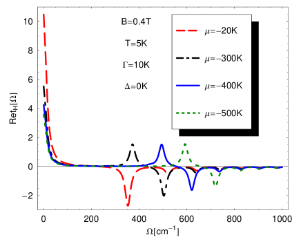
Figure 1: (Color online) Real part of the Hall angle, $\mbox{Re}t_{H}(\Omega)$ at $B=0.4\,\mbox{T}$, temperature $T=5\mbox{K}$, scattering rate $\Gamma=10\,\mbox{K}$ for four values of chemical potential. Long dashed (red) $\mu=-20\,\mbox{K}$, dash-dotted (black) $\mu=-300\,\mbox{K}$, solid (blue) $\mu=-400\,\mbox{K}$, short dashed (green) $\mu=-500\,\mbox{K}$.

In Fig. 1 we show results for the frequency dependence of $\mbox{Re}\,t_{H}(\Omega)$ for a case with external magnetic field $B=0.4\,\mbox{T}$, at temperature $T=5\,\mbox{K}$ and impurity scattering rate $\Gamma=10\,\mbox{K}$. Accordingly, the energies of the Landau levels are $M_{n}=\sqrt{2nL^{2}(B)}$ [see also Eq. (5) in Ref. Gusynin2007JPCM, ]— viz., $M_{1}\simeq 265\,\mbox{K}$, $M_{2}\simeq 375\,\mbox{K}$, $M_{3}\simeq 460\,\mbox{K}$, and $M_{4}\simeq 531\,\mbox{K}$, respectively. Thus the long dashed (red) curve with $\mu=-20\,\mbox{K}$ is for $|\mu|<M_{1}$, the dash-dotted (black) curve with $\mu=-300\,\mbox{K}$ is for $M_{1}<|\mu|<M_{2}$, the solid (blue) line with $\mu=-400\,\mbox{K}$ is for $M_{2}<|\mu|<M_{3}$ and the short dashed (green) curve with $\mu=-500\,\mbox{K}$ is for $M_{3}<|\mu|<M_{4}$. The values chosen for all the parameters used in Fig. 1 are quite reasonable. For a magnetic field $0.4\mbox{T}$ the various Landau energies fall within the range of available optical spectrometers and this is one value of $B$ used in Ref. Sadowski2006, on the optics of several-layer graphite. The value of the broadening parameter $\Gamma$ is not so well known, but our choice is reasonable when compared with the line broadening seen in experiments.Sadowski2006 Higher values would simply broaden the lines seen in Fig. 1. Further in field-effect graphene devices Novoselov2004Science ; Geim2005Nature ; Kim2005Nature the chemical potential can be easily varied from $-3600\,\mbox{K}$ to $3600\,\mbox{K}$ simply by changing the gate voltage. Low temperatures can also be easily achieved. Starting with the long dashed (red) curve of Fig. 1 we notice a Drude-like behavior of $\mbox{Re}\,t_{H}(\Omega)$ at small $\Omega$, followed by a region where it is small. It then changes sign, after which it exhibits a negative peak around $375\,\mbox{cm}^{-1}$. This is followed by a further series of small peaks, all negative, which decay in amplitude as the frequency $\Omega$ increases. The frequencies of the peaks do not correspond to the sum or differences of two adjacent Landau level energies $M_{n}$ as do the peaks in both $\mbox{Re}\,\sigma_{xx}(\Omega)$ and $\mbox{Im}\,\sigma_{xy}(\Omega)$ seen in Ref. Gusynin2007JPCM, . Rather they fall, approximately, at energies between two peaks in $\mbox{Re}\,\sigma_{xx}(\Omega)$ (see Fig. 1 in Ref. Gusynin2007JPCM, taking into account that it is plotted for $B=1\,\mbox{T}$), where the $\mbox{Im}\,\sigma_{xx}(\Omega)$ also crosses zero and the denominator in $\mbox{Re}\,t_{H}=\mbox{Re}(\sigma_{xy}/\sigma_{xx})$ which is equal to $(\mbox{Re}\,\sigma_{xx}(\Omega))^{2}+(\mbox{Im}\,\sigma_{xx}(\Omega))^{2}$ consequently has a minimum. The numerator $\mbox{Re}\,\sigma_{xx}(\Omega)\mbox{Re}\,\sigma_{xy}(\Omega)+\mbox{Im}\,\sigma_{xx}(\Omega)\mbox{Im}\,\sigma_{xy}(\Omega)$ plays little role in the peak positions, but determines their sign which can be positive or negative as seen in the other three curves (for larger values of chemical potential). In this case the first peak is positive and this is followed by, decaying in amplitude, a sequence of higher-energy peaks, all of which are negative. Note that the position of the first positive peak in each of the dash-dotted, solid, and dashed curves moves progressively to higher energy as the chemical potential crosses a new Landau level. This happens because, as we have already stated, the peaks in $\mbox{Re}\,t_{H}(\Omega)$ fall in the between two consecutive peaks in $\mbox{Re}\,\sigma_{xx}(\Omega)$ (for $M_{N}<|\mu|<M_{N+1}$, the first interband peak in $\mbox{Re}\,\sigma_{xx}(\Omega)$ falls at $M_{N}+M_{N+1}$).

Returning to the small-$\Omega$ behavior of $\mbox{Re}\,t_{H}(\Omega)$, where a Drude-like behavior was noted, we see that the weight under this peak is progressively depleted as $\mu$ crosses through larger Landau level energies. These features can be understood qualitatively from approximate expressions for $\mbox{Re}\,t_{H}(\Omega)$ obtained by keeping only the leading term in the formulas for both the longitudinal $\sigma_{xx}(\Omega)$ and Hall $\sigma_{xy}(\Omega)$ conductivity. In Ref. Gusynin2007JPCM, we provided expressions (11) and (12) which we will not repeat here. Both involve a sum over Landau levels $n=0,1,2,\ldots$. If $|\mu|$ falls in the interval $]M_{0},M_{1}[$, retaining only the $n=0$ contribution to the sum, we get for $T=0$

$$\sigma_{xx}(\Omega)=\frac{e^{2}v_{F}^{2}|eB|}{\pi ci}\frac{2(\Omega+2i\Gamma)}{M_{1}}\frac{1}{M_{1}^{2}-(\Omega+2i\Gamma)^{2}}$$ (51)

and

$$\sigma_{xy}(\Omega)=-\frac{e^{2}v_{F}^{2}eB\,\mbox{sgn}\,\mu}{\pi c}\frac{2}{M_{1}^{2}-(\Omega+2i\Gamma)^{2}}.$$ (52)

It follows from Eqs. (52) and (51) that

$$t_{H}(\Omega)=-\frac{i\sqrt{2\hbar|eB|v_{F}^{2}/c}\,\mbox{sgn}\,(eB)\,\mbox{sgn}\,\mu}{\Omega+2i\Gamma},\qquad\mbox{Re}\,t_{H}(\Omega)=-\frac{M_{1}2\Gamma\,\mbox{sgn}\,(eB)\,\mbox{sgn}\,\mu}{\Omega^{2}+4\Gamma^{2}}.$$ (53)

This shows that while $\mbox{Re}\,\sigma_{xx}(\Omega)$ and $\mbox{Im}\,\sigma_{xy}(\Omega)$ are peaked near $\Omega=M_{1}$, the small $\Omega$ limit of $\mbox{Re}\,t_{H}(\Omega)$ is indeed Drude in shape with width $2\Gamma$. Also its height at $\Omega=0$ and $\mu<0$ is $M_{1}/2\Gamma$ which is set by the inverse scattering rate $2\Gamma$ and by the Landau scale $L(B)$, because $M_{1}=\sqrt{2}L(B)$.

On the other hand, for $\mu\in]M_{N},M_{N+1}[$ the first nonzero term in the expression for the Hall angle $t_{H}(\Omega)$ is for $n=N$. Retaining only this contribution to the conductivities (11) and (12) from Ref. Gusynin2007JPCM, and defining

$$A_{N}^{\pm}=\frac{1}{(M_{N+1}\pm M_{N})^{2}-(\Omega+2i\Gamma)^{2}}$$ (54)

for $T=0$ we get

$$\sigma_{xx}(\Omega) = \frac{e^{2}v_{F}^{2}|eB|(\Omega+2i\Gamma)}{\pi ci}\left(\frac{A_{N}^{-}}{M_{N+1}-M_{N}}+\frac{A_{N}^{+}}{M_{N+1}+M_{N}}\right),$$ (55)

$$\sigma_{xy}(\Omega) = -\frac{e^{2}v_{F}^{2}eB}{\pi c}\left(A_{N}^{-}+A_{N}^{+}\right).$$ (56)

Hence for $t_{H}$ we obtain the Drude term

$$t_{H}(\Omega)=-i\frac{\mbox{sgn}\,(eB)\,\mbox{sgn}\,\mu}{\Omega+2i\Gamma}\frac{A_{N}^{-}+A_{N}^{+}}{A_{N}^{-}/(M_{N+1}-M_{N})+A_{N}^{+}/(M_{N+1}+M_{N})}.$$ (57)

It follows directly from this formula that $\mbox{Re}\,t_{H}(\Omega)$ in the limit of large $N$ is given approximately by

$$\mbox{Re}\,t_{H}(\Omega)\cong-\frac{1}{2\sqrt{N}}\frac{M_{1}2\Gamma\,\mbox{sgn}\,(eB)\,\mbox{sgn}\,\mu}{\Omega^{2}+4\Gamma^{2}},\qquad N\gg 1.$$ (58)

The value $\mbox{Re}\,t_{H}(\Omega=0)=M_{1}/(4\sqrt{N}\Gamma)$ is roughly verified in our numerical work, where larger $N$ corresponds to larger chemical potential, and these results serve as a guide to our numerical work.

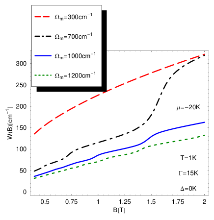
Figure 2: (Color online) Partial Hall spectral weight $W(\Omega_{m})$ as a function of field $B$ at $\mu=-20\,\mbox{K}$, temperature $T=1\,\mbox{K}$, scattering rate $\Gamma=15\mbox{K}$ for four values of $\Omega_{m}$. Long dashed (red) $\Omega_{m}=300\,\mbox{cm}^{-1}$, dash-dotted (black) $\Omega_{m}=700\,\mbox{cm}^{-1}$, solid (blue) $\Omega_{m}=1000\,\mbox{cm}^{-1}$, short dashed (green) $\Omega_{m}=1200\,\mbox{cm}^{-1}$.

Our theory predicts not only the position in energy of the various lines as well as the shape of the $\mbox{Re}\,t_{H}(\Omega)$ at small photon energy, but also provides values for the optical spectral weight under the various features seen in Fig. 1. Information on this spectral weight is conveniently presented in terms of the partial sum rule of Eq. (50) for typical values of the cutoff $\Omega_{m}$ as a function of the magnetic field. In Fig. 2 we show numerical results for the Hall angle spectral weight $W(\Omega_{m})$ in $\mbox{cm}^{-1}$ as a function of the value of the external magnetic field $B$ for four values of the cutoff $\Omega_{m}$ at fixed value of $\mu=-20\,\mbox{K}$, $T=1\,\mbox{K}$ and $\Gamma=15\,\mbox{K}$. For the long dashed (red) curve with the cutoff $\Omega_{m}=300\,\mbox{cm}^{-1}$ only the frequency region in the long dashed (red) curve of Fig. 1 which falls below the first peak (negative in this case) in $\mbox{Re}\,t_{H}(\Omega)$ is integrated in the weight. While in Fig. 1 the field $B=0.4\,\mbox{T}$, the peaks in $\mbox{Re}\,t_{H}(\Omega)$ move to higher energies as $B$ increases and so for all values of $B$ used in the figure only the Drude region around small $\Omega$ of the curve is integrated over. Using the formula (53) as a rough approximation we expect in this case $W(\Omega_{m})$ to scale as the square root of $B$ coming from the $M_{1}$ factor. This is verified to good accuracy in the numerical work. When $\Omega_{m}$ increases, as is the case for the other three curves of Fig. 2, the peaks in $\mbox{Re}\,t_{H}(\Omega)$, which are negative for $\mu=-20\,\mbox{K}$, start entering the integral and this reduces the value of the optical sum. However, we have no simple approximate analytic formula which might capture the essence of the situation in this case, so we must rely on the numerical work. It is also clear that for a given value of $B$, the reduction in the optical sum caused by the negative peaks in $\mbox{Re}\,t_{H}(\Omega)$ will be less as $B$ increases, because the peaks move to higher energies. In fact the upward steps, seen most clearly in the dash-dotted (black) curve of Fig. 2 with the cutoff $\Omega_{m}=700\,\mbox{cm}^{-1}$, correspond to values of $B$ for which a peak in $\mbox{Re}\,t_{H}(\Omega)$ is starting to fall outside the integration range. The first step occurs around $B\sim 0.75\,\mbox{T}$ when the second negative peak in the long dashed curve of Fig. 1 is moving through $700\,\mbox{cm}^{-1}$, while for $B\sim 1.6\,\mbox{T}$ it is the first peak in $\mbox{Re}\,t_{H}(\Omega)$ which is involved. This peak is larger in absolute value and so this second step is larger. Note also that in this case the dash-dotted (black) curve merges with the long dashed (red) curve for the smaller cutoff as it must, since in both instances only the Drude-like contribution at small $\Omega$ is relevant to the integral.

Another feature of the curves in Fig. 2 is worth commenting on. We note that the short dashed (green) curve for $\Omega_{m}=1200\,\mbox{cm}^{-1}$ becomes linear in $B$ at small $B$ in contrast to the long dashed (red) curve which, as we saw, went like $\sqrt{B}$. We can get some understanding of this crossover which corresponds to the case when many peaks are involved in the integration, by considering the $B\to 0$ limit. In Ref. Gusynin2007JPCM, we also obtained the expressions (13) for $\sigma_{xx}$ and (14) for $\sigma_{xy}$ which for $\Delta=0$ read

$$\begin{split}\sigma_{xx}(\Omega)=-&\frac{2ie^{2}(\Omega+2i\Gamma)}{h}\left[\frac{1}{(\Omega+2i\Gamma)^{2}}\int_{0}^{\infty}d\omega|\omega|\left(\frac{\partial n_{F}(\omega)}{\partial\omega}-\frac{\partial n_{F}(-\omega)}{\partial\omega}\right)\right.\\ &-\left.\int_{0}^{\infty}d\omega\frac{n_{F}(-\omega)-n_{F}(\omega)}{(\Omega+2i\Gamma)^{2}-4\omega^{2}}\right]\end{split}$$ (59)

and

$$\begin{split}\sigma_{xy}(\Omega)=&\frac{e^{2}v_{F}^{2}eB}{\pi c}\int_{0}^{\infty}d\omega\left(\frac{\partial n_{F}(\omega)}{\partial\omega}+\frac{\partial n_{F}(-\omega)}{\partial\omega}\right)\\ &\times\left[-\frac{1}{(\Omega+2i\Gamma)^{2}}+\frac{1}{4\omega^{2}-(\Omega+2i\Gamma)^{2}}\right].\end{split}$$ (60)

For $T=0$ we get

$$\sigma_{xx}(\Omega) = \frac{2ie^{2}}{h}\left[\frac{|\mu|}{\Omega+2i\Gamma}+\frac{1}{4}\ln\frac{2|\mu|-(\Omega+2i\Gamma)}{2|\mu|+(\Omega+2i\Gamma)}\right],$$ (61)

$$\sigma_{xy}(\Omega) = \frac{e^{2}v_{F}^{2}eB}{\pi c}\mbox{sgn}\mu\left[\frac{1}{(\Omega+2i\Gamma)^{2}}+\frac{1}{(\Omega+2i\Gamma)^{2}-4\mu^{2}}\right].$$ (62)

Hence for $|\mu|\gg\Omega,\Gamma$ we obtain

$$t_{H}(\Omega)=-\frac{\hbar v_{F}^{2}eB}{c\mu}\frac{1}{2\Gamma-i\Omega}=-\frac{\hbar eB\,\mbox{sgn}\,\mu}{cm_{c}}\frac{1}{2\Gamma-i\Omega},$$ (63)

where in the second equality we introduced the cyclotron mass $m_{c}$. This form is to be contrasted to that obtained in Eq. (53) for large magnetic field $B$, where $t_{H}(\Omega)$ is proportional to $\sqrt{B}$ rather than to $B$ as in Eq. (63). Except for a sign change this result is of the same form as in Eq. (22) of Ref. Drew1997PRL, with $m_{c}$ playing the role of mass which in graphene varies as the square root of the carrier imbalance $|\rho|$Geim2005Nature ; Kim2005Nature . Here we emphasize the linear dependence on magnetic field $B$ in Eq. (63) as well as in the full sum rule (4) with $\omega_{H}$ given by Eq. (46).

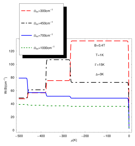
Figure 3: (Color online) Partial Hall spectral weight $W(\Omega_{m})$ as a function of $\mu$ at $B=0.4\,\mbox{K}$, temperature $T=1\,\mbox{K}$, scattering rate $\Gamma=15\mbox{K}$ for four values of $\Omega_{m}$. Long dashed (red) $\Omega_{m}=300\,\mbox{cm}^{-1}$, dash-dotted (black) $\Omega_{m}=450\,\mbox{cm}^{-1}$, solid (blue) $\Omega_{m}=700\,\mbox{cm}^{-1}$, short dashed (green) $\Omega_{m}=1000\,\mbox{cm}^{-1}$.

An experimental configuration which has already been used by Li et al. in Ref. Basov-organic, is incorporating the specimen into a field-effect deviceNovoselov2004Science ; Geim2005Nature ; Kim2005Nature . In this case the chemical potential $\mu$ is easily changed by varying the gate voltage. In Fig. 3 we show numerical results for $W(\Omega_{m})$ in $\mbox{cm}^{-1}$ as a function of chemical potential $\mu$ in K for four values of the cutoff $\Omega_{m}$. The magnetic field $B$ has been set to $0.4\,\mbox{T}$, $T=1\,\mbox{K}$, and $\Gamma=15\,\mbox{K}$. We see steps occurring in these curves as the chemical potential $\mu$ crosses the Landau level energies – viz., $M_{1}\simeq 265\,\mbox{K}$, $M_{2}\simeq 375\,\mbox{K}$, $M_{3}\simeq 460\,\mbox{K}$ and $M_{4}\simeq 531\,\mbox{K}$, respectively. Between successive sharp rises, $W(\Omega_{m})$ stays nearly constant quite independent of $\mu$. The long dashed (red) curve has the smallest cutoff equal to $300\,\mbox{cm}^{-1}$ which falls below the first peak in the long dashed (red) curve of Fig. 1 for $\mu=-20\,\mbox{K}$ and its value $\sim 135\,\mbox{cm}^{-1}$ corresponds to the area under the Drude part of the curve (in Fig. 1). Remaining with $\Omega_{m}=300\,\mbox{cm}^{-1}$ as $|\mu|$ is increased beyond $M_{1}$ but is less than $M_{2}$, the value of $W(\Omega_{m})$ decreases. This now corresponds to the dash-dotted (black) curve of Fig. 1 which has a smaller Drude-like piece than does the long dashed (red) curve and the drop is close to a factor of $0.56$ while our simplified but analytic formula (58) predicts $0.71$ (which is better than can be expected as it is valid only for $N\gg 1$ and we are using it outside the range of validity). The dash-dotted (black) curve has $\Omega_{m}=450\,\mbox{cm}^{-1}$ which is chosen to fall above the first (negative) peak in the long dashed (red) curve of Fig. 1. For $|\mu|<M_{1}$ the dash-dotted curve of Fig. 1 applies, and to get $W(\Omega_{m})$, we are integrating through the first negative peak in addition to the Drude-like peak centered at $\Omega=0$. This reduces its value to about half the value it had for the lower cutoff $\Omega_{m}=300\,\mbox{cm}^{-1}$. In the region $\mu\in]M_{1},M_{2}[$, however, the dash-dotted curve of Fig. 1 applies and we are integrating over the first positive peak in $\mbox{Re}\,t_{H}(\Omega)$ as well as through the Drude-like region and so the value of the weight $W(\Omega_{m})$ is now increased. After this it decreases again as more negative peaks are integrated over. The other two curves can be understood as well with arguments similar to those used for the first two cutoffs.

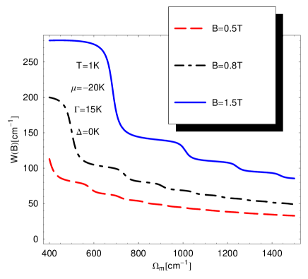
Figure 4: (Color online) Partial Hall spectral weight $W(\Omega_{m})$ as a function of the cutoff $\Omega_{m}$ at $\mu=-20\,\mbox{K}$, $T=1\,\mbox{K}$, scattering rate $\Gamma=15\mbox{K}$ for three values of $B$. Long dashed (red) $B=0.5\,\mbox{T}$, dash-dotted (black) $B=0.8\,\mbox{T}$, solid (blue) $B=1.5\,\mbox{T}$.

Finally in Fig. 4 we present results for $W(\Omega_{m})$ as a function of $\Omega_{m}$ for $T=1\,\mbox{K}$, $\Gamma=15\,\mbox{K}$, and $\mu=-20\,\mbox{K}$ for three values of magnetic field. Each curve shows steps as the various peaks beyond the Drude-like structure in $\mbox{Re}\,t_{H}(\Omega)$ vs $\Omega$ are included in the integral defining $W(\Omega_{m})$ as $\Omega_{m}$ is increased. These steps are most pronounced for the solid (blue) curve with $B=1.5\,\mbox{T}$. For this field value the peaks in the long dashed curve of Fig. 1 will be shifted upwards by a factor of $\sim 1.94$, so that the first drop corresponds to integrating over the first negative peak in the equivalent of the the long dashed (red) curve of Fig. 1, while the second drop corresponds to integrating over the second negative peak etc. The drops in the other curves can be similarly traced and fall at smaller values of $\Omega_{m}$ because of the $\sqrt{B}$ scaling of the peak positions in $\mbox{Re}\,t_{H}(\Omega)$ vs $\Omega$. To end we note that $W(\Omega_{m})$ could also show upward rather than downward steps if we had chosen a larger value of $|\mu|$ between $M_{1}$ and $M_{2}$. In this case as an example, the first peak in $\mbox{Re}\,t_{H}(\Omega)$ is positive, so it adds to the low $\Omega$ Drude-like contribution.

VI Conclusion

We have studied the modification of the usual optical sum rules brought about by the particular band structure of graphene – namely, its compensated semimetal aspects and the Dirac nature of its quasiparticles. The existence of two bands within the same Brillouin zone leads to interband as well as intraband optical transitions both of which enter the optical sums.

We considered both the usual $f$-sum rule on the real part of the longitudinal conductivity $\sigma_{xx}(\Omega)$ and an equivalent sum rule recently introduced by Drew and Coleman Drew1997PRL involving the Hall conductivity. From a formal point of view we find that care must be used in introducing the electromagnetic vector potential. It should be introduced into the initial Hamiltonian through a Peierls phase factor rather than after the diagonalization. The $f$-sum rule is shown to be proportional to $\sim-0.39$ of the kinetic energy per atom rather than the usual minus one-half value, familiar for a square lattice with nearest-neighbor hopping only. This difference reflects the particularity of the honeycomb lattice with nearest-neighbor hopping between the two distinct $A$ and $B$ sublattices.

For small chemical potential $|\mu|<<T$, the longitudinal sum rule displays a $T^{3}$ temperature law rather than conventional $T^{2}$ law of free electron theory. Also for $|\mu|\gg T$ we predict a $|\mu|^{3}$ dependence on chemical potential for the deviation from the $T=\mu=0$ reference case. The first temperature correction in this case goes as $|\mu|T^{2}$, recovering the $T^{2}$ law of free electron theory. The $|\mu|^{3}\varpropto|V_{g}|^{3/2}$ dependence should be observable in field-effect devices.

The sum rule for the Hall conductivity involves the real part $\mbox{Re}\,t_{H}(\Omega)$ of the Hall angle (3). Its integral (4) is equal to the Hall frequency $\omega_{H}$, and in the free electron metals $\omega_{H}$ coincides with the cyclotron frequency. For graphene we find instead that $\omega_{H}$ is given by Eq. (46). Although this equation can be formally written in the form (47) which involves the “relativistic” cyclotron mass $m_{c}=|\mu|/v_{F}^{2}$, expression (47) is different from the conventional one. There are two modifications. The cyclotron mass $m_{c}$ varies as the square root of the carrier density, and $\omega_{H}$ in Eq. (47) is also proportional to the ratio $(\mu/t)^{3}$.

In our previous paper Gusynin2007JPCM we considered partial spectral weight $W_{xx}(\Omega_{m})$ given by Eq. (49) for $\mbox{Re}\,\sigma_{xx}(\Omega)$ and found steplike structures corresponding to peaks in $\mbox{Re}\,\sigma_{xx}(\Omega)$. Here we considered the partial spectral weight $W(\Omega_{m};B,\mu)$ given by Eq. (50) for $\mbox{Re}\,t_{H}(\Omega)$. Interesting steplike structures are also found in which the steps can go up or down depending on the variable used to display the weight $W(\Omega_{m};B,\mu)$. Specifically we analyzed its dependence on the value of the external magnetic field $B$ and chemical potential for various fixed values of $\Omega_{m}$. We also considered the dependence of $W(\Omega_{m};B,\mu)$ on $\Omega_{m}$ for fixed $\mu$ and $B$ values. The rich pattern of behavior can be traced back to the frequency dependence of $\mbox{Re}\,t_{H}(\Omega)$ which shows a Drude-like peak at small $\Omega$ followed by a series of peaks which fall at some energy between the interband peaks of $\sigma_{xx}(\Omega)$, where both its real and imaginary parts are small. Also the peaks in $\mbox{Re}\,t_{H}(\Omega)$ depend on the sign and value of chemical potential.

We hope that these specific predictions for the behavior of $\mbox{Re}\,t_{H}(\Omega)$, the corresponding partial spectral weight $W(\Omega_{m};B,\mu)$, and the sum rules can be verified experimentally.

Appendix A Diamagnetic term

Substituting the Fourier transform (16) into Eq. (12) and summing over the lattice sites, we obtain

$$\begin{split}\sum_{\mathbf{n}}\tau_{\alpha\beta}(\mathbf{n})&=-\frac{te^{2}}{\hbar^{2}}\sum_{\boldsymbol{\delta},\sigma}\delta_{\alpha}\delta_{\beta}\int_{BZ}\frac{d^{2}{\mathbf{k}}}{(2\pi)^{2}}\left[a_{\sigma}({\mathbf{k}})^{\dagger}e^{i\mathbf{k}\boldsymbol{\delta}}b_{\sigma}({\mathbf{k}})+\mbox{h.c.}\right]\\ &=\frac{e^{2}}{\hbar^{2}}\sum_{\sigma}\int_{BZ}\frac{d^{2}{\mathbf{k}}}{(2\pi)^{2}}\left[\frac{\partial^{2}\phi(\mathbf{k})}{\partial k_{\alpha}\partial k_{\beta}}\Upsilon_{\sigma}^{\dagger}(\mathbf{k})\sigma_{+}\Upsilon_{\sigma}(\mathbf{k})+\frac{\partial^{2}\phi^{\ast}(\mathbf{k})}{\partial k_{\alpha}\partial k_{\beta}}\Upsilon_{\sigma}^{\dagger}(\mathbf{k})\sigma_{-}\Upsilon_{\sigma}(\mathbf{k})\right].\end{split}$$ (64)

Accordingly the thermal average $\langle\tau_{\alpha\beta}\rangle$ is easily expressed in terms of the GF (20) as

$$\begin{split}\langle\tau_{\alpha\beta}\rangle=&\frac{2Ve^{2}}{\hbar^{2}}\int_{BZ}\frac{d^{2}{\mathbf{k}}}{(2\pi)^{2}}T\sum_{n=-\infty}^{\infty}e^{-i\omega_{n}\tau}\\ &\times\left[\mbox{tr}[\sigma_{+}G(i\omega_{n},\mathbf{k})]\frac{\partial^{2}\phi(\mathbf{k})}{\partial k_{\alpha}\partial k_{\beta}}+\mbox{tr}[\sigma_{-}G(i\omega_{n},\mathbf{k})]\frac{\partial^{2}\phi^{\ast}(\mathbf{k})}{\partial k_{\alpha}\partial k_{\beta}}\right],\qquad\tau\to 0.\end{split}$$ (65)

Calculating the trace we obtain for the diagonal component of the stress tensor $\langle\tau_{\alpha\beta}\rangle=\langle\tau_{\alpha\alpha}\rangle\delta_{\alpha\beta}$ that

$$\frac{\langle\tau_{\alpha\alpha}\rangle}{V}=-\frac{2e^{2}T}{\hbar^{2}}\sum\limits_{n=-\infty}^{\infty}\int_{BZ}\frac{d^{2}{\bf k}}{(2\pi)^{2}}\frac{1}{(\omega_{n}-i\mu)^{2}+\epsilon^{2}(\mathbf{k})}\left(\phi(\mathbf{k})\frac{\partial^{2}}{\partial k_{\alpha}^{2}}\phi^{\ast}(\mathbf{k})+\mbox{c.c.}\right).$$ (66)

The sum over the Matsubara frequencies converges irrespectively of infinitesimally small $\tau$, and we find

$$\frac{\langle\tau_{\alpha\alpha}\rangle}{V}=\frac{e^{2}}{\hbar^{2}}\int_{BZ}\frac{d^{2}{\bf k}}{(2\pi)^{2}}\frac{1}{2\epsilon(\mathbf{k})}\left[n_{F}\left(\epsilon(\mathbf{k})\right)-n_{F}\left(-\epsilon(\mathbf{k})\right)\right]\left(\phi(\mathbf{k})\frac{\partial^{2}}{\partial k_{\alpha}^{2}}\phi^{\ast}(\mathbf{k})+\mbox{c.c.}\right).$$ (67)

Writing $\phi(\mathbf{k})=\epsilon(\mathbf{k})e^{i\varphi(\mathbf{k})}$ we can recast the last equation in the form (30). The derivatives in the brackets in Eq. (67) are easily calculated using the explicit expression for $\phi(\mathbf{k})$:

$$\phi(\mathbf{k})\frac{\partial^{2}}{\partial k_{\alpha}^{2}}\phi^{\ast}(\mathbf{k})+\mbox{c.c.}=\frac{1}{2}\sum_{\alpha=1,2}\left(\phi(\mathbf{k})\frac{\partial^{2}}{\partial k_{\alpha}^{2}}\phi^{\ast}(\mathbf{k})+\mbox{c.c.}\right)=-\frac{a^{2}}{3}\epsilon^{2}(\mathbf{k}).$$ (68)

Substituting Eq. (68) into Eq. (67) we arrive at the final expression (31).

Appendix B Hall term

Here we calculate the commutator $I_{x,y}=\langle[J_{x}(t=0),J_{y}(t=0)]\rangle$ of the paramagnetic currents $J_{x}(t=0)$ and $J_{y}(t=0)$ that are defined in Eq. (23). Since this commutator is nonzero only in the presence of a magnetic field, the corresponding current density operator $j_{a}(\mathbf{n})$ has to be taken for a finite vector potential $\mathbf{A}$:

$$j_{a}(\mathbf{n})=-\frac{ite}{\hbar}\sum_{\boldsymbol{\delta},\sigma}\delta_{a}\left[a_{\mathbf{n},\sigma}^{\dagger}T_{\boldsymbol{\delta}}b_{\mathbf{n},\sigma}-b_{\mathbf{n},\sigma}^{\dagger}T_{-\boldsymbol{\delta}}a_{\mathbf{n},\sigma}\right],$$ (69)

where the operator

$$T_{\boldsymbol{\delta}}=e^{i\boldsymbol{\delta}(\mathbf{p}+e/c\mathbf{A})/\hbar}.$$ (70)

Using the anticommutation relations for $a_{\mathbf{n},\sigma}$ and $b_{\mathbf{n},\sigma}$ operators we calculate the commutator

$$[j_{x}(\mathbf{n}),j_{y}(\mathbf{m})]=\frac{e^{2}t^{2}\delta_{nm}}{\hbar^{2}}\sum_{\boldsymbol{\delta},\boldsymbol{\delta}^{\prime},\sigma}\delta_{x}\delta_{y}^{\prime}\left\{a_{\mathbf{n},\sigma}^{\dagger}\left(T_{\boldsymbol{\delta}}T_{-\boldsymbol{\delta}^{\prime}}-T_{\boldsymbol{\delta}^{\prime}}T_{-\boldsymbol{\delta}}\right)a_{\mathbf{n},\sigma}+b_{\mathbf{n},\sigma}^{\dagger}\left(T_{-\boldsymbol{\delta}}T_{\boldsymbol{\delta}^{\prime}}-T_{-\boldsymbol{\delta}^{\prime}}T_{\boldsymbol{\delta}}\right)b_{\mathbf{n},\sigma}\right\}.$$ (71)

Provided that the magnetic flux per unit cell is far less than a flux quantum $h/e$, we may expand the operator $T_{\boldsymbol{\delta}}$

$$T_{\boldsymbol{\delta}}\approx 1+i\frac{\delta_{a}}{\hbar}\left(p_{a}+\frac{e}{c}A_{a}\right).$$ (72)

Then using the commutator

$$[D_{a},D_{b}]\equiv\left[p_{a}+\frac{e}{c}A_{a},p_{b}+\frac{e}{c}A_{b}\right]=-i\frac{e\hbar}{c}B\epsilon_{ab},\qquad a,b=1,2$$ (73)

we obtain

$$T_{\boldsymbol{\delta}}T_{-\boldsymbol{\delta}^{\prime}}-T_{\boldsymbol{\delta}^{\prime}}T_{-\boldsymbol{\delta}}=\frac{1}{\hbar^{2}}[\delta_{a}\delta_{b}^{\prime}D_{a}D_{b}-\delta_{a}^{\prime}\delta_{b}D_{a}D_{b}]=\frac{\delta_{a}\delta_{b}^{\prime}}{\hbar^{2}}(-i)\frac{e\hbar}{c}B\epsilon_{ab},$$ (74)

where the sum over the dummies $a,b$ is implied. Now the sum over $\boldsymbol{\delta},\boldsymbol{\delta}^{\prime}$ in Eq. (71) can be evaluated as follows

$$\sum_{\boldsymbol{\delta},\boldsymbol{\delta}^{\prime}}\delta_{x}\delta_{y}^{\prime}\delta_{\gamma}\delta_{\kappa}^{\prime}\epsilon_{\gamma\kappa}=\epsilon_{\gamma\kappa}\sum_{\boldsymbol{\delta}}\delta_{x}\delta_{\gamma}\sum_{\boldsymbol{\delta}^{\prime}}\delta_{y}^{\prime}\delta_{\kappa}^{\prime}=\epsilon_{xy}\frac{a^{4}}{4},$$ (75)

where in the second equality we used the relation

$$\sum_{\lambda=1,2,3}(\delta_{\lambda})_{\alpha}(\delta_{\lambda})_{\beta}=\frac{a^{2}}{2}\delta_{\alpha\beta}.$$ (76)

Substituting the commutator (71) into the expression $I_{x,y}=\sum_{\mathbf{n},\mathbf{m}}\langle[j_{x}(t=0,\mathbf{n}),j_{y}(t=0,\mathbf{m})]\rangle$ and utilizing Eqs. (74) and (75) we arrive at the representation

$$I_{x,y}=-i\frac{e^{2}a^{4}t^{2}\hbar eB}{4\hbar^{4}c}\epsilon_{xy}\sum_{\mathbf{n},\sigma}\langle(a_{\mathbf{n},\sigma}^{\dagger}a_{\mathbf{n},\sigma}+b_{\mathbf{n},\sigma}^{\dagger}b_{\mathbf{n},\sigma})\rangle.$$ (77)

Thus to complete the calculation of $I_{x,y}$ we have to find the thermal average

$$\tilde{I}\equiv\sum_{\mathbf{n},\sigma}\langle(a_{\mathbf{n},\sigma}^{\dagger}a_{\mathbf{n},\sigma}+b_{\mathbf{n},\sigma}^{\dagger}b_{\mathbf{n},\sigma})\rangle.$$ (78)

As in Appendix A, $\tilde{I}$ is expressed in terms of the GF (20) as

$$\tilde{I}=\sum_{\mathbf{n}}\sum_{\sigma}\mbox{tr}[\hat{I}G_{\sigma}(\tau,\mathbf{0})]=2VT\sum_{n}\int_{BZ}\frac{d^{2}{\mathbf{k}}}{(2\pi)^{2}}[G_{11}(i\omega_{n},\mathbf{k})+G_{22}(i\omega_{n},\mathbf{k})]e^{-i\omega_{n}\tau},$$ (79)

where

$$G_{11}(i\omega_{n},\mathbf{k})=G_{22}(i\omega_{n},\mathbf{k})=\frac{1}{2}\left[\frac{1}{i\omega_{n}+\mu-\epsilon(\mathbf{k})}+\frac{1}{i\omega_{n}+\mu+\epsilon(\mathbf{k})}\right]$$ (80)

are the diagonal in the sublattice space components of the GF (20). In contrast to the convergent Matsubara sums (65) and (66) in the off-diagonal components of the GF (20), regularization of the Matsubara sum (79) by the factor $e^{-i\omega_{n}\tau}$ is crucial, because it would diverge otherwise. The factor $e^{-i\omega_{n}\tau}$ regularizes the sum over Matsubara frequencies differently depending on the sign of $\tau$:

$$\lim_{\tau\to\pm 0}T\sum\frac{e^{-i\tau\omega_{n}}}{i\omega_{n}+\mu-\omega}=-\frac{1}{2}[1-2n_{F}(\omega)]-\frac{\mbox{sgn}\tau}{2}=\left\{\begin{array}[]{lr}n_{F}(\omega),&\tau\to-0,\\ n_{F}(\omega)-1,&\tau\to+0.\\ \end{array}\right.$$ (81)

Normally to count the number of particles Abrikosov.book one takes the limit $\tau\to-0$. One can check, however, that such a prescription leads to a contradiction when calculating the integral (79), because it results in $\tilde{I}$ which is not odd in $\mu$, while the LHS of Eq. (4) is odd in $\mu$. This contradiction is resolved if one takes into account that the first term of the GF (80) describes electrons, so that the prescription $\tau\to-0$ has to be used, while the second term of the GF (80) describes holes and the prescription $\tau\to+0$ is necessary. Then we obtain

$$\tilde{I}=2V\int_{BZ}\frac{d^{2}{\mathbf{k}}}{(2\pi)^{2}}[n_{F}(\epsilon(\mathbf{k}))+n_{F}(-\epsilon(\mathbf{k}))-1],$$ (82)

which is odd in $\mu$. The quantity (82) describes the carrier imbalance $\rho=n_{e}-n_{h}$, where $n_{e}$ and $n_{h}$ are the densities of electrons and holes, respectively. It was considered in the Dirac approximation in Appendix C of Ref. Gusynin2006PRB, , and here we use two expressions (44) and (48) for $\rho$.

References

• (1) J.E. Hirsch, Physica C 199, 305 (1992); ibid. 201, 347 (1992).
• (2) A. J. Millis, in Strong Interactions in Low Dimensions, edited by D. Baeriswyl and L. De Giorgi (Kluver Academic, Berlin, 2003).
• (3) D. van der Marel, Interaction electrons in low dimensions, book series Physics and Chemistry of Materials with Low- Dimensional Structures (Kluwer Academic, Berlin, 2003); cond-mat/0301506 (unpublished).
• (4) L. Benfatto and S. Sharapov, Fiz. Nizk. Temp. 32, 700 (2006) [Low Temp. Phys. 32, 533 (2006).]
• (5) J.P. Carbotte and E. Schachinger, J. Low Temp. Phys. 144, 61 (2006).
• (6) H.D. Drew and P. Coleman, Phys. Rev. Lett. 78, 1572 (1997).
• (7) K.S. Novoselov, A.K. Geim, S.V. Morozov, D. Jiang, Y. Zhang, S.V. Dubonos, I.V. Grigorieva, and A.A. Firsov, Science 306, 666 (2004); K.S. Novoselov, D. Jiang, T. Booth, V.V. Khotkevich, S.M. Morozov, A.K. Geim, Proc. Nat. Acad. Sc. 102, 10451 (2005).
• (8) K.S. Novoselov, A.K. Geim, S.V. Morozov, D. Jiang, M.I. Katsnelson, I.V. Grigorieva, S.V. Dubonos, A.A. Firsov, Nature 438, 197 (2005).
• (9) Y. Zhang, Y.-W. Tan, H.L. Stormer, P. Kim, Nature 438, 201 (2005).
• (10) A.K. Geim and K.S. Novoselov, Nature Materials 6, 183 (2007).
• (11) A.H. Castro Neto, F. Guinea, and N.M. Peres, Physics World 19, 33 November (2006).
• (12) P.R. Wallace, Phys. Rev. 77, 622 (1947).
• (13) G.W. Semenoff, Phys. Rev. Lett. 53, 2449 (1984).
• (14) D.P. DiVincenzo and E.J. Mele, Phys. Rev. B 29, 1685 (1984).
• (15) J. González, F. Guinea, and M.A.H. Vozmediano, Nucl. Phys. B 406, 771 (1993).
• (16) V.P. Gusynin, S.G. Sharapov and J.P. Carbotte, Phys. Rev. Lett. 96, 256802 (2006).
• (17) V.P. Gusynin, S.G. Sharapov and J.P. Carbotte, J. Phys.: Condens. Matter. 19, 026222 (2007); cond-mat/0607727.
• (18) L.A. Falkovsky and A.A. Varlamov, cond-mat/0606800.
• (19) Y. Zheng and T. Ando, Phys. Rev. B 65, 245420 (2002).
• (20) V.P. Gusynin and S.G. Sharapov, Phys. Rev. B 73, 245411 (2006).
• (21) S.G. Sharapov, V.P. Gusynin, and H. Beck, Phys. Rev. B 69, 075104 (2004).
• (22) V.P. Gusynin and S.G. Sharapov, Phys. Rev. B 71, 125124 (2005).
• (23) B.S. Shastry, B.I. Shraiman, and R.R.P. Singh, Phys. Rev. Lett. 70, 2004 (1993).
• (24) L. Lewin, Polylogarithms and Associated Functions (Elsevier, North-Holland, Amsterdam, 1981).
• (25) L.B. Rigal, D.C. Schmadel, H.D. Drew, B. Maiorov, E. Osquigil, J.S. Preston, R. Hughes, and G.D. Gu, Phys. Rev. Lett. 93, 137002 (2004).
• (26) M.L. Sadowski, G. Martinez, M. Potemski, C. Berger, and W.A. de Heer, Phys. Rev. Lett. 97, 266405 (2006).
• (27) Z.Q. Li, S.-W. Tsai, W.J. Padilla, S.V. Dordevic, K.S. Burch, Y.J. Wang, and D.N. Basov, Phys. Rev. B 74, 195404 (2006).
• (28) J. Hwang, T. Timusk, and G.D. Gu, J. Phys.: Condens. Matter. 19, 125208 (2007)
• (29) N. Bontemps, cond-mat/0610307, to appear in Physica C.
• (30) Z.Q. Li, G.M. Wang, N. Sai, D. Moses, M.C. Martin, M. Di Ventra, A.J. Heeger, and D.N. Basov, Nano Letters 6, 224 (2006).
• (31) A.A. Abrikosov, L.P. Gorkov, and I.E. Dzyaloshinski, Methods of Quantum Field Theory in Statistical Physics (Dover, New York, 1975).
Refer to caption