Collisional properties of sympathetically cooled ³⁹K

Abstract

We report the experimental evidence of the sympathetic cooling of ³⁹K with ⁸⁷Rb down to $1\,\mu$K, obtained in a novel tight confining magnetic trap. This allowed us to perform the first direct measurement of the elastic cross section of ³⁹K below $50\,\mu$K. The result obtained for the triplet scattering length, $a_{T}=-51(7)$ Bohr radii, agrees with previous results derived from photoassociation spectra and from Feshbach spectroscopy of ⁴⁰K.

I Introduction

In the field of ultracold and quantum gases Potassium gained a key role since it is the only alkali, beside Lithium, for which a stable fermionic isotope exists. Furthermore, since the sympathetic cooling of fermionic ⁴⁰K with ⁸⁷Rb, the most widespread atom in the laboratories devoted to laser cooling, is particularly favorable, it is not surprising that so many experiments with ultracold fermions were carried out or are planned with this atom. In contrast very little attention was paid to the two other (bosonic) isotopes of Potassium, ³⁹K and ⁴¹K. These isotopes offer the possibility of creating double species Bose-Einstein condensates, which display rich and interesting quantum phase diagrams when trapped in optical lattices Altman et al. (2003); Isacsson et al. (2005); Chen and Wu (2003); Zheng et al. (2005). After the seminal work where a double species ⁴¹K-⁸⁷Rb BEC was produced in a magnetic trap Modugno et al. (2002), essentially no experiments have addressed these topics.

Along these guidelines, we started an experiment devoted to the exploration of degenerate Bose-Bose mixtures in optical lattices. In this work we report that also ³⁹K can be sympathetically cooled with ⁸⁷Rb although this is much more difficult due to its unfavorable laser cooling and scattering properties, thus demonstrating that all the stable isotopes of Potassium can be cooled to ultralow temperatures.

Laser cooling of ³⁹K has several disadvantages if compared to alkalis such as ⁸⁷Rb or even ⁴⁰K. These disadvantages are related to the hyperfine structure of the $P_{3/2}$ level whose separation is of the same order of magnitude as the natural linewidth of the cooling transition $|F=2,m_{F}=+2\rangle\rightarrow|F=3,m_{F}=+3\rangle$. The resulting strong optical pumping towards the $|F=1\rangle$ manifold must be countered by a repumping light with an intensity comparable to that of the light driving the cooling transition. A careful balance of the intensity and the detuning of these two laser frequencies, unsuitable for optimized loading of a Magneto-Optical-Trap (MOT), is the only way to obtain temperatures at the Doppler limit by laser cooling Fort et al. (1998). Furthermore, the s-wave elastic cross section of ³⁹K at zero temperature is more than one order of magnitude smaller than that of ⁸⁷Rb and, due to the attractive character of the interaction, the Ramsauer-Townsend minimum Mott and Massey (1965) occurs at a temperature of around $320\,\mu$K where the contribution of other partial waves is still small Simoni (2006). All these features strongly hamper the efficiency of evaporative cooling. Note that, due to Pauli blocking, an even more dramatic decrease in the evaporative cooling efficiency occurs for the fermionic ⁴⁰K.

For these reasons the most widely employed experimental technique to reach ultralow temperatures in a K gas is sympathetic cooling with ⁸⁷Rb. This amounts to producing a mixed MOT of the two species and then evaporatively cool ⁸⁷Rb allowing K to thermalize with it. With this technique it has been possible to reach quantum degeneracy of ⁴⁰K DeMarco and Jin (1999) and ⁴¹K Modugno et al. (2001), but no attempts have been made to test this method on ³⁹K. For this mixture in fact, the inter-species cross section is again more than one order of magnitude smaller than the one of ⁸⁷Rb-⁴⁰K and ⁸⁷Rb-⁴¹K Ferlaino et al. (2006a, b).

We demonstrate here for the first time that ³⁹K can be sympathetically cooled to $1\,\mu$K. Therefore the work presented in this paper is a critical step towards the production of a Bose-Einstein Condensate (BEC) of ³⁹K. Such a system is a promising candidate for the realization of a BEC with interaction tunable around zero, since a broad Feshbach resonance is predicted around $400\,$G Ferlaino et al. (2006a, b).

The achievement of sympathetic cooling allowed us to perform the first direct measurement of the s-wave elastic cross section of ³⁹K. Assuming from earlier work on photoassociation spectra Wang et al. (2000) and on Feshbach spectroscopy of ⁴⁰K Loftus et al. (2002) the attractive character of the interatomic interaction (i.e. the negative sign of the s-wave scattering length), our results agrees with Wang et al. (2000); Loftus et al. (2002) within $1.7$ combined standard deviations.

The time required for sympathetic cooling depends crucially on the collision rate between the two species. If this time is of the same order of magnitude as the lifetime of the sample, the density will drop during the evaporation and cooling will eventually stop. Since the cross section for ³⁹K-⁸⁷Rb collision is smaller than in the case of ⁴⁰K and ⁴¹K, one has to increase the lifetime of the sample and/or the confinement before starting sympathetic cooling. In the experiments reported here, the confinement of the ³⁹K sample is increased by more than a factor $2$ with respect to Modugno et al. (2002) employing a new kind of magneto-static trap of size intermediate between micro-traps, where microscopic current-carrying wires are laid on a chip, and traditional magnetic traps created with multiple winding coils Wang et al. (2006).

The outline of the paper is the following: in section II we will present a brief description of the experimental apparatus and the results about sympathetic cooling of ⁸⁷Rb and ³⁹K. In section III we will introduce the experimental procedure for studying ultracold collision in ³⁹K and we will present the theoretical analysis of the data. Finally, we will conclude with the perspectives of ⁸⁷Rb- ³⁹K evaporative cooling and of a ³⁹K BEC.

II Experimental Apparatus

II.1 Laser system and MOT loading

In order to provide the maximum flexibility for the loading of the mixed MOT, our experimental apparatus features two distinct two-dimensional MOT’s (2D-MOT) for the separate precooling of ⁸⁷Rb and ³⁹K. A complete description of our laser system and a thorough characterization of our ³⁹K 2D-MOT can be found in Ref. Catani et al. (2006). The 2D-MOT employed for ⁸⁷Rb has exactly the same structure and similar performances. In the experiments we used $130\,(110)$ mW for the cooling light and $40\,(6)$ mW of repumping light for ³⁹K (⁸⁷Rb). The atomic flux provided by the two 2D-MOT’s is collected inside a mixed MOT formed in a ultra high vacuum chamber. The MOT is formed by a standard configuration with six independent laser beams with $25$ mm diameter and a total power of $45\,(40)$ mW for the cooling light and $24\,(6)$ mW for the repumping light of ³⁹K (⁸⁷Rb). These beams are split from the output of one single mode fiber in which we inject the four different frequencies needed for the two species, thereby guaranteeing a perfect geometric overlap of the cooling and repumping light and of the two MOT’s. The magnetic field gradient of about $16\,$G/cm used in the MOT is provided by a pair of anti-Helmholtz coils operating at $4\,$A.

We typically load around $2\times 10^{9}$ atoms of ⁸⁷Rb and $5\times 10^{6}$ atoms of ³⁹K in $10$ and $1$ s respectively. We can control very precisely the number of ³⁹K atoms loaded in the MOT adjusting the time of operation of the 2D-MOT. After the loading of the MOT we reduce the repumping intensity and increase the magnetic field gradient to compress the cloud, we apply a $3.5\,$ms stage of polarization-gradient cooling, optically pump the atoms of both species towards the $|F=2,m_{F}=+2\rangle$ state and then trap them in a purely magnetic trap.

II.2 Magnetic trap and evaporation

Our magnetic trap represents a compromise between the usual magnetic traps generated by coils placed outside the vacuum system, typically low confining ($\nu_{\mathrm{max}}\sim 100\,$Hz), high power consuming ($\sim 1\,$kW), several centimeters in size, which produce the largest BEC’s ($>10^{6}$ atoms), and the so called microtraps operating in vacuum, providing a high confinement ($\nu_{\mathrm{max}}\sim 1$ kHz), requiring low electrical power ($\sim 1\,$W), that easily fit on a microchip, but usually produce smaller condensates ($\sim 10^{4}$ atoms).

The potential generated by our trap is of the Ioffe-Pritchard type and the structure has both current conductors laying on a chip and free standing Wang et al. (2006). The free standing conductors are built from a single oxygen-free copper tube machined to form the four Ioffe bars and two partial rings that provide the end caps of the potential in the axial direction. The axial confinement is increased by a circular copper trace laid on a direct-bond copper chip that interfaces the current leads and the free standing conductors. Electrical and mechanical contact between the parts is obtained by vacuum brazing and the current leads are brought outside the Ultra-High Vacuum environment by a custom-made electrical feedthrough. To allow optical access along the horizontal axial direction, the feedthrough is hollow and terminates with a vacuum viewport; optical access in the radial direction is easily obtained through the $2$ mm gaps between the Ioffe bars. Since these gaps are too small to allow the efficient production of a MOT, the magnetic trap, hereafter called millimetric-trap or mTrap, is displaced by $26$ mm from the center of the MOT. A big coil placed outside vacuum is used to adjust the bias field of the trap thereby changing the radial confinement. The confinement provided by our mTrap at $95$ A current and $6$ G bias field is $\omega_{r}=2\pi\times 447(7)$ Hz and $\omega_{z}=2\pi\times 29.20(1)$Hz for ³⁹K.

The displacement of the atoms from the MOT position to the mTrap is accomplished holding them inside a quadrupole trap which is moved with a motorized translation stage. The quadrupole trap is formed ramping the current of the MOT coils up to $65$ A and the motion takes less than $500$ ms in order to reduce the losses due to Majorana spin-flip.

While the magnetic field of the mTrap adds to that of the transfer trap along the radial directions, along the axial direction the mTrap generates a field directed in the opposite direction so that an adiabatic transfer of atoms would be only possible decreasing the trap depth during the process and therefore reducing the number of transferred atoms. To overcome this potential pitfall we employ a mixed approach to load the trap: we ramp up the current of the mTrap in $150\,$ms, a time which is fully adiabatic only for the radial direction. The overall efficiency of the transfer from the MOT to the mTrap is around 30%, and we typically trap $7\times 10^{8}$ ⁸⁷Rb and $4\times 10^{5}$ ³⁹K atoms.

Once atoms are loaded inside the magnetic trap we perform evaporation on the ⁸⁷Rb cloud by transferring the hottest atoms to the antitrapped $|F=1,m_{F}=+1\rangle$ state with a microwave sweep around 6.8 GHz. In addition we apply a second ramp to remove unwanted atoms from the $|F=2,m_{F}=+1\rangle$ level. The ³⁹K is unaffected by these sweeps, owing to the huge difference in frequency with the corresponding hyperfine transition (460 MHz), and only minor losses occur during the evaporation. Provided that the number of ⁸⁷Rb atoms $N_{Rb}$ at a given temperature is still larger than the initial number of ³⁹K atoms $N_{K}$, the former can act as coolant establishing thermal equilibrium, as it is shown in Fig. 1. For this reason the initial number of ³⁹K atoms is reduced in the pictures from $2.7\times 10^{5}$ in the first picture to $5.9\times 10^{4}$ of the last one at a temperature of $1.0(1)\,\mu$K.

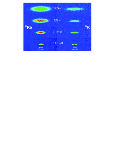
Figure 1: (Color online) Experimental sequence showing sympathetic cooling between ⁸⁷Rb (left) and ³⁹K (right). All the images are taken after $1$ ms expansion. The phase space density at $1\,\mu$K is $0.02$ and $0.01$. Images are taken along the vertical radial direction.

We experimentally found that a sufficient condition to reach thermal equilibrium is $N_{Rb}/N_{K}>2.7$, but no attempt has been made to measure the inter-species elastic cross section since it can be obtained with high precision from the results of Feshbach spectroscopy of the ⁴⁰K-⁸⁷Rb mixture Ferlaino et al. (2006a, b). We used instead the known value $a_{K-Rb}=+36a_{0}$ to guide the optimization of the evaporation. Indeed we experimentally verified that in presence of ³⁹K atoms, in order to optimize the number of ⁸⁷Rb atoms below a few $\mu$K, the evaporation ramp must be slowed down in the last part to be sure that the two species are always in thermal equilibrium.

III Cross-thermalization measurement

III.1 Introduction

We measure the cross section of ³⁹K by analyzing the relaxation of the atomic cloud towards thermal equilibrium. The technique can be described as follows. The dynamics of an ideal gas isolated and confined in an harmonic potential is completely separable meaning that the different spatial degrees of freedom are decoupled. If such a sample is prepared with different energy distributions along different directions this difference will not vary with time. On the other hand, due to interactions, the collisions drive the system towards thermal equilibrium, namely a state in which the total energy is conserved and the effective temperatures of the different degrees of freedom are equal. If the initial state has different effective temperatures, the relaxation towards thermal equilibrium can provide direct information on the collisions. In our system this is accomplished in the following way: after obtaining a cloud of cold ³⁹K as described in Section II, ⁸⁷Rb is blowed away from the trap with a pulse of resonant light and the radial degrees of freedom of K are excited by parametric excitation, obtained modulating the value of the trap bias field at the frequency of radial confinement for $100$ ms. Due to our elongated trap geometry this excitation is highly selective and the axial degree of freedom maintains its effective temperature. Following this excitation we allow the cloud to relax for a time $t_{w}$ after which we image the cloud along the vertical radial direction by means of in situ absorption imaging. From the measured widths $w$ of the Gaussian density profile we can calculate the average potential energy along the radial ($r$) and axial ($z$) direction as

$$E_{i}=\frac{1}{2}k_{B}T_{i}=\frac{m}{2}(\omega_{i}w_{i})^{2}\quad i=r,z\,\,.$$ (1)

where $m$ is the atomic mass. Repeating this measurement for different $t_{w}$ allows us to measure the relaxation of the ratio between the axial and radial temperatures. As shown in Fig. 2 this is well fitted by an exponential decay. The time constant $\tau$ of this decay is related to the elastic scattering cross section and to the density of the sample by the following relation:

$$\tau^{-1}=\frac{\gamma_{el}}{\alpha}=\frac{\bar{n}\langle\sigma v\rangle}{\alpha},$$ (2)

where $\alpha$ is the number of collisions required to an atom to reach thermal equilibrium, $\gamma_{el}$ is the intraspecies collision rate for ³⁹K, $\bar{n}$ is the average density, $\sigma$ is the scattering cross section, $v$ is the relative velocity of two colliding atoms and $\langle\cdot\rangle$ indicates averaging over the velocity distribution in the cloud.

If one indicates the geometric average of the temperature along the different direction as $\bar{T}=(T_{r}^{2}T_{z})^{1/3}$ and introduces an average, temperature-dependent cross section defined as:

$$\tilde{\sigma}(\bar{T})=\frac{\langle\sigma v\rangle}{\langle v\rangle}\qquad,$$ (3)

since the average density of a harmonic trap is:

$$\bar{n}=\left(\frac{m}{4\pi k_{B}\bar{T}}\right)^{3/2}N_{K}\omega_{r}^{2}\omega_{z}$$ (4)

and the average relative velocity is $\langle v\rangle=4\,(k_{B}\bar{T})^{1/2}\,(\pi m)^{-1/2}$, the relaxation rate can be expressed as:

$$\tau^{-1}=\frac{\gamma_{el}}{\alpha}=\frac{\tilde{\sigma}(\bar{T})}{\alpha}\,N_{K}\,\frac{m\omega_{r}^{2}\omega_{z}}{2\pi^{2}k_{B}\bar{T}}.$$ (5)

We will come back to the relation between $\tilde{\sigma}$ and the actual energy-dependent cross-section in Sec. III.3.

Eq. (5) holds only if one assumes that the average density of the sample does not change during the relaxation process. Actually the loss rate induced by collisions with atoms of the background gas is about $0.03\,\mathrm{s}^{-1}$ for the experiments reported in this work. If this rate is not negligible as compared to the measured relaxation rates, it must be taken into account: one expects that the reduction of the density slows down the relaxation so that after an initial decay with a rate corresponding to Eq. (5), equilibrium apparently sets for a value of $E_{z}/E_{r}$ lower than $1$. This picture is further complicated by the unavoidable heating rate present in the experiment that increases the temperature throughout the measurements: in our system we measure a different heating rate in the axial and radial direction so that it is possible to achieve equilibrium also for a value of $E_{z}/E_{r}$ greater than $1$.

In principle, one could take these effects into account having the equilibrium value of the energy ratio as a free parameter: for our measurements however the equilibrium value is almost always consistent with $1$. We therefore choose to fix it to $1$ in order to improve the estimation of the time constant, as it is shown in Fig. 2.

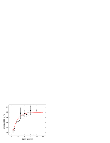
Figure 2: (Color online) Plot of the relaxation dynamics of an ultracold sample of ³⁹K after parametric heating in the radial direction. Data are taken after expansion (see text). Each point is an average of several experimental realization and the line is an exponential decay fit with equilibrium value fixed to $1$, initial value and time constant as free parameters. Average initial number of atoms is $379(10)\times 10^{3}$ and initial average temperature is $16.2(7)\,\mu$K. From the fit we obtain $\tau=3.66(46)\,$s.

III.2 Measurements of the elastic cross section

In order to reduce systematic errors on the determination of $\tilde{\sigma}$, we performed several measurements at different densities and for two different temperatures of $29$ and $16\,\mu$K. Furthermore, to check that the inhomogeneous magnetic field present in our in situ imaging was not a source of error, the dataset at $16\,\mu$K is taken with a slightly different procedure. First, we adiabatically decompress the trap to $\omega_{r}=2\pi\times 290(1)\,$Hz and $\omega_{z}=2\pi\times 21.24(1)\,$Hz and then blow away ⁸⁷Rb, apply parametric heating at $\omega_{r}$, wait for a variable time and image the cloud after a $2\,$ms expansion.

The results of our measurements are shown in Fig. 3 where we report the relaxation rate $\gamma=\tau^{-1}$ as a function of the initial number of atoms $N_{K}$. Figure 3(a) shows the measurements taken after expansion with an average initial temperature $\bar{T}=16(1)\,\mu$K, while Fig. 3(b) presents measurements taken in situ with $\bar{T}=28.9(1.3)\,\mu$K. One can see that the relaxation rate has the expected linear dependence on the number of atoms and the extrapolation towards zero is consistent with zero.

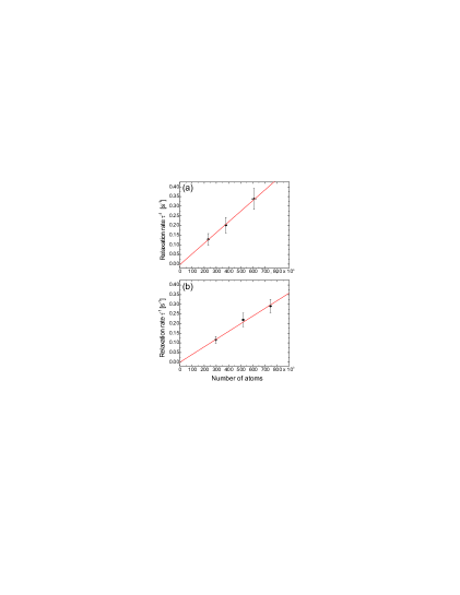
Figure 3: (Color online) Plot of the measured relaxation rate as a function of the number of atoms in the sample after expansion (a) and in situ (b). The measured initial average temperature is $16(1)\,\mu$K and $28.9(1.3)\,\mu$K respectively. The slope of the linear fit to the data is related to the elastic cross-section, while the intercept is a measure of ergodic mixing as described in the text. The fit results are: $\gamma_{mix}=-0.003(0.065)\,\mathrm{s}^{-1}$ and $A=5.5(1.6)\times 10^{-7}\,\mathrm{s}^{-1}$ for figure (a) and $\gamma_{mix}=-0.0005(0.034)\,\mathrm{s}^{-1}$ and $A=4.0(1.0)\times 10^{-7}\,\mathrm{s}^{-1}$ for figure (b). Error bars on the vertical direction are statistical error on the exponential decay fit, while on the horizontal direction they are the statistical fluctuation of the initial number of atoms not including the calibration uncertainty.

In a Ioffe-Pritchard trap, a sufficiently big atomic cloud can experience a potential that is not strictly separable so that different degrees of freedom are coupled and relaxation can occur even in the absence of collisions. We refer to this process as ergodic mixing. A priori, for equal harmonic frequencies, ergodic mixing could play a more prominent role in our mTrap than in the usual traps due to its small size. For this reason we take ergodic mixing into account by separating the component of the relaxation rate, which is linear in $N$, from the extrapolation in the limit of zero density where relaxation can only occur through ergodic mixing. One can therefore assume that

$$\gamma=\alpha^{-1}\frac{\mathrm{d}\gamma_{el}}{\mathrm{d}N_{K}}N_{K}+\gamma_{mix}=AN_{K}+\gamma_{mix}\qquad,$$ (6)

where $\gamma_{mix}$ is the time constant of the ergodic mixing process. The two parameters $A$ and $\gamma_{mix}$ are obtained from a linear fit of the experimental data, as shown in Fig. 3. By using Eq. (5) one has

$$A=\frac{\tilde{\sigma}}{\alpha}\,\frac{m\omega_{r}^{2}\omega_{z}}{2\pi^{2}k_{B}\bar{T}}\qquad.$$ (7)

As pointed out above, since the values for $\gamma_{mix}$ are consistent with zero in both the datasets, we can conclude that ergodic mixing plays a negligible role in our measurements.

The resulting values for the temperature-dependent average elastic cross section, computed from Eq. (7) with $\alpha=2.7$, as obtained from numerical simulation described in Sec. III.4, are $2.2(0.8)\times 10^{-12}\,\mathrm{cm}^{2}$ and $0.91(0.22)\times 10^{-12}\,\mathrm{cm}^{2}$ for $16$ and $29\,\mu$K respectively. These values are a very good approximation of the actual cross section as we show in the next section.

III.3 Extracting the value of the scattering length

As pointed out above, the measured cross sections depend on the temperature. In order to extract information on the interatomic potential, one has to make some assumption on the behavior of the cross section as a function of temperature. A simple partial wave expansion of the scattering amplitude shows that, for the experimental condition reached in this work, collisions can only occur at $l=0$ angular momentum, odd values being suppressed on symmetry ground and even values due to the low temperature . In a very general form the s-wave cross section for identical boson is:

$$\sigma(k) = 8\pi|f_{0}(k)|^{2}$$ (8)

where $k=mv/(2\hbar)$ is the relative wavevector and $f_{0}(k)$ is the s-wave scattering amplitude that can be expressed in terms of the S-matrix phase shift $\delta_{0}(k)$: $f_{0}(k)=e^{i\delta_{0}(k)}\sin\delta_{0}(k)/k$.

In the limit of vanishing energy, given that the potential decays more rapidly than $1/r^{3}$, we can express the cross section as a function of a single parameter, the s-wave scattering length which, for two alkali atom in the stretched $|F=2,m_{F}=+2\rangle$ state, is the triplet one $a_{T}$ :

$$|f_{0}(k)|^{2} \simeq a^{2}_{T}$$ (9)

$$\sigma(k) \simeq 8\pi a^{2}_{T}$$ (10)

For higher temperature one has to calculate the scattering amplitude up to order $k^{2}:f_{0}(k)=(-1/a_{T}+ik+\frac{1}{2}k^{2}r_{e}+\dots)^{-1}$, where $r_{e}$ denotes the effective range, which is a function of the scattering length $a_{T}$ and the $C_{6}$ coefficient of the van der Waals potential Flambaum et al. (1999)

$$\sigma(k)=8\pi\frac{a^{2}_{T}}{(1-\frac{1}{2}k^{2}r_{e}a_{T})^{2}+k^{2}a_{T}^{2}}.$$ (11)

Since the $C_{6}$ coefficients are well known for all alkali dimers Derevianko et al. (2001); Ticknor et al. (2004), we numerically invert Eq. (3) after inserting Eq. (11), averaging over the Boltzmann thermal distribution and assuming $a_{T}<0$, to obtain the scattering length: $a_{T}=-67(11)a_{0}$ from data at $16\,\mu$K and $a_{T}=-48(5)a_{0}$ from data at $29\,\mu$K . For comparison, we notice that, if we neglect the effective range, these values would be $-57(11)a_{0}$ and $-36(5)a_{0}$, respectively. In the first case the two values differ by approximately 1.57 combined standard deviations, while in the second case the difference is 1.75. The quoted uncertainties derive mainly from the fits of Fig. 3 and the atom number calibration ($\pm 20\%$), which was done independently for each data set. Finally, we take a weighted average of the two scattering length values calculated with effective range and multiply the associated uncertainty by a factor $\sqrt{\chi^{2}}=1.65$, to set the confidence level to 68% Brandt (1998): the result is $a_{T}=-51(7)a_{0}$.

Prior to this work, the ³⁹K triplet s-wave scattering length has been measured by photoassociation spectroscopy, $a_{T}=-33(5)a_{0}$ Wang et al. (2000), and by mass-scaling from rethermalization of ⁴⁰K, $a_{T}=-37(6)a_{0}$ Loftus et al. (2002). Indeed our measurement is the first direct determination of the elastic cross section for this isotope. To different extents, all reported values of the scattering length depend on the $C_{6}$ coefficient of the van der Waals long range potential: we take $C_{6}=3927\,$a.u. Ticknor et al. (2004), while in Ref. Wang et al. (2000); Loftus et al. (2002) $C_{6}$ is assumed equal to $3897\,$a.u. Derevianko et al. (2001). We checked that our value changes with $C_{6}$ with a rate $\delta|a_{t}|=0.001a_{0}\times\delta C_{6}$ [a.u.], approximatively $50$ times smaller than in Ref. Wang et al. (2000) (no such rate is available in Ref. Loftus et al. (2002)) and therefore the difference in the $C_{6}$ does not significantly change the derived scattering length. As our result differs from the average of the published values of $1.70$ combined standard deviation, we conclude that the agreement is satisfactory.

III.4 Numerical simulations

As shown in Eq. (7), to compute the value of the scattering length from the fit to the data one needs to know the value of the parameter $\alpha$, which is the average number of collisions per particle needed for thermalization. This parameter depends on the temperature and the trap frequencies in a non trivial way and can vary from 2.4 to 3.4 Dalibard (1998). Following Monroe et al. (1993); Arndt et al. (1997); Wu and Foot (1996) we estimate this parameter from a numerical simulation of the system. Taking advantage of the low density and small atom number of the sample, we make a direct simulation of the gas in which we consider 3D position and velocity of every single atom. Choosing a time step $\delta t$ much smaller than both the average collision time $\gamma_{coll}^{-1}$ and the faster timescale of single particle dynamics, namely $\omega_{r}^{-1}$, one may assume that during the time interval $\delta t$ interactions between atoms are weak enough that they decouple with the center of mass motion and that the force experienced by the atoms varies little. Therefore the dynamics of the gas can be directly simulated with the following procedure:

1. Position and velocity are updated according to external forces with a Verlet integrator.

2. Every $M$ steps, the positions of the atoms in real space are discretized on a lattice of spacing $\delta x$ and if two atoms are located at the same site a collision test is made.

3. If the collision test is positive, the collision is resolved using simple classical mechanics and s-wave scattering:

   $$\left\{\begin{array}[]{c}\mathbf{v}_{1}^{\prime}=\mathbf{v}_{CM}+\frac{|\mathbf{v}_{r}|}{2}\,\hat{\mathbf{e}}_{R}\\ \mathbf{v}_{2}^{\prime}=\mathbf{v}_{CM}-\frac{|\mathbf{v}_{r}|}{2}\,\hat{\mathbf{e}}_{R}\end{array}\right.$$

   where $\mathbf{v}_{i}^{\prime}$ indicates the velocity of particle $i$ after the collision, $\mathbf{v}_{CM}$ and $\mathbf{v}_{r}$ are the center of mass and relative velocity respectively, before the collision, and $\hat{\mathbf{e}}_{R}$ is a random direction on the unit sphere.

The collision test consists in comparing a random real number $y$, uniformly distributed in $\left[0,1\right)$, with the collision probability calculated according to kinetic theory:

$$\wp=\sigma\,|v_{r}|\,M\,\delta t\,\delta x^{-3}$$ (12)

where $\sigma$ is the elastic scattering cross section and $|v_{r}|$ is the modulus of the relative velocity; collision is processed if $y<\wp$. In order to reproduce a correct scattering rate, one must choose $\delta x$ so that the average number of atoms in a volume $\delta x^{3}$ is much smaller than $1$ and $M$ so that the distance traveled by an atom during the time $M\,\delta t$ is of the order of $\delta x$.

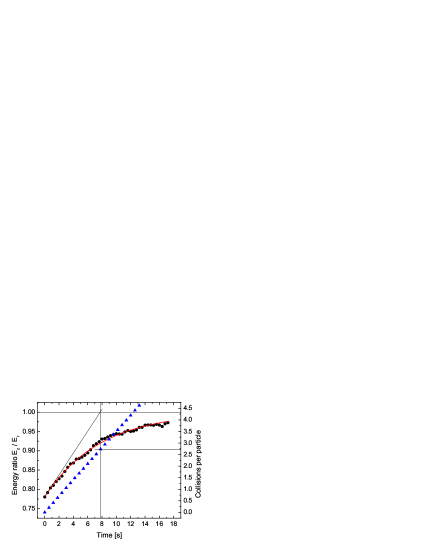
Figure 4: (Color online) Plot of the simulated energy ratio (black dots, left scale) and collisions per particle (blue triangles, right scale) as a function of time for $20\times 10^{3}$ atoms in a harmonic trap whose frequencies are $440$ and $29.4\,$Hz in the radial and axial direction respectively. The red curve is an exponential decay fit. The value $\alpha=2.72$ can be obtained directly from the graph identifying the time constant of the decay ($7.74$ s).

In Fig. 4 we report a typical result of the simulation showing the radial to axial energy ratio and the number of collisions per atom as a function of time. The simulation is performed in a cylindrical harmonic trap with radial and axial frequency of $440$ and $29.4\,$Hz respectively. The number of atoms is $2\times 10^{4}$ and the initial energy distribution has a width of $15(19.5)\,\mu$K along the axial (radial) direction. The cross section is $8.6\times 10^{-16}\,\mathrm{m}^{2}$ so that the scattering rate in the simulation is close to the experimental one. The value of $\alpha=2.7$ can be extracted directly from the graph as explained in the caption of Fig. 4.

IV Conclusions

In summary we have demonstrated sympathetic cooling of ³⁹K with ⁸⁷Rb, in spite of the low interspecies cross section, and we have measured the cross section for elastic collision between two ³⁹K atoms in a pure triplet state. We have hence obtained the triplet s-wave scattering length $a_{T}$, assuming its negative sign and an effective range approximation for the s-wave scattering amplitude at low but finite temperature.

The possibility of sympathetic cooling and the knowledge of the collisional properties of bosonic potassium open the way to its use as a quantum degenerate gas. Bosonic potassium isotopes, ³⁹K and ⁴¹K, are predicted to feature Feshbach resonances, several Gauss wide, at moderate fields ($<1$ kG). As a consequence, optically trapped bosonic potassium appears a suitable candidate to realize a condensate with a scattering length tunable around zero. Such a condensate would be interesting for interferometric purposes, as the interaction energy limits the accuracy of interferometers employing Bose-Einstein condensates. In addition, wide Feshbach resonances make potassium condensates particularly attractive to realize double condensates in optical lattices, for quantum simulation purposes. For ³⁹K, in particular, Bohn and coworkers have predicted a Feshbach resonance around $40$ G for two atoms in the $|F=1,m_{F}=-1\rangle$ state, with a width of several tens of Gauss Bohn et al. (1999), while another 60 G broad resonance has been predicted around 400 G for atoms in the absolute ground state $|F=1,m_{F}=1\rangle$ Simoni and Tiesinga (2006). While a double condensate of ⁴¹K and ⁸⁷Rb was produced in a magnetic trap Modugno et al. (2002), ³⁹K has not been brought to degeneracy so far. This work represents a decisive step in this direction as we reached a phase-space density of $0.01$, with a gain of several orders of magnitude with respect to the state-of-the-art Fort et al. (1998).