String correlation functions of the spin-1/2 Heisenberg XXZ chain

Abstract

We calculate certain string correlation functions, originally introduced as order parameters in integer spin chains, for the spin-1/2 XXZ Heisenberg chain at zero temperature and in the thermodynamic limit. For small distances, we obtain exact results from Bethe Ansatz and exact diagonalization, whereas in the large-distance limit, field-theoretical arguments yield an asymptotic algebraic decay. We also make contact with two-point spin-correlation functions in the asymptotic limit.

1 Introduction

Haldane’s work [1, 2] on the different ground-state properties of integer-$S$ and half-integer-$S$ spin chains triggered efforts to seek for a quantitative understanding of the gapped ground state of integer-$S$ chains. Among these are the works of den Nijs and Rommelse [3] as well as Oshikawa [4], where the following generalized string correlation function was considered:

$$\mathcal{O}(n,\theta) \equiv -4\left\langle S_{1}^{z}\exp\left[{\rm i}\theta\sum_{k=2}^{n-1}S_{k}^{z}\right]S_{n}^{z}\right\rangle.$$ (1.1)

The authors of [3] introduced $\lim_{n\to\infty}\mathcal{O}(n,\pi)$ as an order parameter that characterizes the gapped ground state for the $S=1$ Heisenberg chain and acquires a non-zero value there. Kennedy and Tasaki [5] introduced a transformation showing that this is due to a broken hidden $Z_{2}\times Z_{2}$ symmetry of the model. In [4], an attempt was made to generalize this argument to integer $S>1$ chains. In the same reference, the den Nijs-Rommelse order parameter was considered for $\theta\neq\pi$. Several subsequent works considered the generalized string correlation functions (1.1) for integer spin ${S>1}$ and generic $\theta$, where $\lim_{n\to\infty}\mathcal{O}(n,\theta)$ acquires non-zero values. The exact calculation for the Valence Bond Solid (VBS) state shows that the correlation takes its maximum values near ${\theta=\pi/S}$ [4, 6].

Whereas in these works, the focus was mainly on integer spin chains motivated by Haldane’s conjecture, interest at the same time rose for $\mathcal{O}(n,\pi)$ in half-integer spin chains. Hida [7] studied $\mathcal{O}(n,\pi)$ for alternating spin-1/2 systems, as this model describes a crossover between the gapped $S=1$ phase and the isotropic spin-1/2 Heisenberg chain. In that paper, he reported the asymptotic form of $\mathcal{O}(n,\pi)\sim\mbox{const. }n^{-1/4}$ close to the uniform, isotropic spin-1/2 chain by means of a field-theoretical approach (the constant was not known there). This means that the string correlation function for the spin-1/2 Heisenberg chain $\mathcal{O}(n,\pi)$ decays in an algebraic way much slower than the usual spin-spin correlation function.

Recently, a related string correlation function

$$\rho(n,\theta) \equiv \left\langle\exp\left[{\rm i}\theta\sum_{k=1}^{n}S_{k}^{z}\right]\right\rangle$$ (1.2)

was introduced by Lou et al.[8]. They came to the conclusion that asymptotically, for spin $S=3/2$, $\left.\mathcal{O}(n,\theta)\right|_{S=3/2}\sim-\sin^{2}(\theta/2)\,\left.\rho(n,\theta)\right|_{S=1/2}$. This means that the scaling behaviour of $\left.\rho(n,\theta)\right|_{S=1/2}$ is also important for $S=3/2$, which is supported by the fact that the spin-3/2 and spin-1/2 chains are considered to belong to the same universality class [9, 10]. Using a field-theoretical approach, the authors of [8] found $\left.\rho(n,\theta)\right|_{S=1/2}\sim\mbox{const. }n^{-\theta^{2}/(4\pi^{2})}$ with an unspecified constant, again for the isotropic spin-1/2 chain.

As far as two-point correlation functions of the spin-1/2 chain are concerned, enormous progress has been made in the last decade to obtain exact expressions from Bethe Ansatz [11, 12, 13] for short distances [14, 15, 16, 17, 18, 19, 20, 21, 22, 23, 24, 25, 26, 27, 28] and from field-theory for both the amplitudes and the exponents of the leading terms in the asymptotic limit [29, 30, 31, 32]. These results are not restricted to the isotropic point, but cover the critical anisotropic regime as well,

$$H=J\sum_{l=1}^{N}\left(S^{x}_{l}S^{x}_{l+1}+S^{y}_{l}S^{y}_{l+1}+\Delta S^{z}_{l}S^{z}_{l+1}\right),$$ (1.3)

with periodic boundary conditions and $J>0$. In the following, we use the anisotropy parameter $\gamma$ to parameterize the anisotropy $\Delta=:\cos\gamma$, with $0<\gamma<\pi$, such that the isotropic points $\gamma=0,\pi$ are excluded.

Given those technical tools from Bethe Ansatz and field theory, in this work we calculate $\rho(n,\theta)$ and $\mathcal{O}(n,\theta)$, both for short distances and in the asymptotic limit. We thus obtain the exponents and the amplitudes of the leading uniform and alternating parts and verify them by the Bethe Ansatz results. Interestingly, the leading asymptotics of the alternating part can be directly obtained from those of the uniform part. We furthermore study the limiting values $\theta\to 0,1-\gamma/\pi$ in the asymptotic limit, where contact is made with $\langle S^{z}_{1}S^{z}_{n}\rangle$ and $\langle S^{x}_{1}S^{x}_{n}\rangle$.

This article is organized as follows. In the next section, we present the Bethe Ansatz calculation of $\rho(n,\theta)$ and $\mathcal{O}(n,\theta)$, as well as results from exact diagonalization that we obtained additionally. The third part contains the field-theoretical approach. Numerical comparisons between the Bethe Ansatz and field-theoretical results are included in an appendix. Calculations not immediately necessary for the understanding of the main text are deferred to further appendices.

2 Exact short distance string correlation functions

The Hamiltonian (1.3) has been solved exactly by the Bethe Ansatz [11, 12, 13]. In fact the eigenfunctions can be constructed in a form of superposition of plane waves, which are called the Bethe Ansatz wave functions. The corresponding eigenenergies are obtained by solving the Bethe Ansatz equations

$$\mbox{e}^{{\rm i}k_{j}N}=(-1)^{M-1}\prod_{l\neq j}\displaystyle{\frac{\mbox{e}^{{\rm i}(k_{j}+k_{l})}+1-2\Delta e^{{\rm i}k_{j}}}{\mbox{e}^{{\rm i}(k_{j}+k_{l})}+1-2\Delta\mbox{e}^{{\rm i}k_{l}}}},\ \ \ \ \ \ \ \ \ \ \ \ \ \ \ \ (j=1,...,M),$$ (2.4)

where ${M}$ is the number of the down spins. With a solution of the Bethe Ansatz equations (2.4), the corresponding eigenenergy is expressed as

$$E=\frac{JN\Delta}{4}+J\sum_{j=1}^{M}\left(\cos k_{j}-\Delta\right).$$ (2.5)

Especially the ground state is given by a solution in the sector ${M=N/2}$. In the critical region ${-1<\Delta=\cos\gamma<1}$, its value per site in the thermodynamic limit ${N\to\infty}$ becomes

$$e_{0}=\frac{J\Delta}{4}-\frac{J\sin\gamma^{2}}{4}\int_{-\infty}^{\infty}\frac{{\rm d}x}{(\cosh\gamma x-\cos\gamma)\cosh\pi x/2}$$ (2.6)

Enormous works have been contributed to evaluate the physical quantities of the model based on the Bethe Ansatz equations (2.4) [13]. They, however, are usually limited to the bulk quantities. Especially, the exact calculation of correlation functions still is a difficult problem. Only for ${\Delta=0}$, where the system reduces to a lattice free-fermion model after a Jordan-Wigner transformation, arbitrary correlation functions can be calculated by means of Wick’s theorem [35, 36]. Especially, the two-point spin-spin correlation function is simply given by ${\langle S_{j}^{z}S_{j+k}^{z}\rangle=-\left(1-(-1)^{k}\right)/(2\pi^{2}k^{2})}$.

There have been many attempts to evaluate the correlation functions for general ${\Delta}$. However, explicit exact evaluations of the correlation functions have become attainable only recently. For example, the following exact values for the spin-spin correlation functions ${\langle S_{j}^{z}S_{j+k}^{z}\rangle}$, were obtained up to ${k=7}$ for ${\Delta=1}$ [24] and up to ${k=8}$ for ${\Delta=1/2}$ [37]:

• ${\Delta=1}$

  $$\langle S_{j}^{z}S_{j+1}^{z}\rangle = \frac{1}{12}-\frac{1}{3}\ln 2=-0.147715726853315\cdots,$$

  $$\langle S_{j}^{z}S_{j+2}^{z}\rangle = \frac{1}{12}-\frac{4}{3}\ln 2+\frac{3}{4}\zeta(3)=0.060679769956435\cdots,$$

  $$\langle S_{j}^{z}S_{j+3}^{z}\rangle = \frac{1}{12}-3\ln 2+\frac{37}{6}\zeta(3)-\frac{14}{3}\ln 2\cdot\zeta(3)-\frac{3}{2}\zeta(3)^{2}$$

  $$-\frac{125}{24}\zeta(5)+\frac{25}{3}\ln 2\cdot\zeta(5)=-0.0502486272572352\cdots,$$

  $$\langle S_{j}^{z}S_{j+4}^{z}\rangle = \frac{1}{12}-\frac{16}{3}\ln 2+\frac{145}{6}\zeta(3)-54\ln 2\cdot\zeta(3)-\frac{293}{4}\zeta(3)^{2}$$

  $$-\frac{875}{12}\zeta(5)+\frac{1450}{3}\ln 2\cdot\zeta(5)-\frac{275}{16}\zeta(3)\cdot\zeta(5)-\frac{1875}{16}\zeta(5)^{2}$$

  $$+\frac{3185}{64}\zeta(7)-\frac{1715}{4}\ln 2\cdot\zeta(7)+\frac{6615}{32}\zeta(3)\cdot\zeta(7)$$

  $$= 0.0346527769827281\cdots,$$

  $$\langle S_{j}^{z}S_{j+5}^{z}\rangle = -0.0308903666476093\cdots,$$

  $$\langle S_{j}^{z}S_{j+6}^{z}\rangle = 0.0244467383279589\cdots,$$

  $$\langle S_{j}^{z}S_{j+7}^{z}\rangle = -0.0224982227633722\cdots.$$ (2.7)

• ${\Delta=1/2}$

  $$\langle S_{j}^{z}S_{j+1}^{z}\rangle = -\frac{1}{8}=-0.125,$$

  $$\langle S_{j}^{z}S_{j+2}^{z}\rangle = \frac{7}{256}=0.02734375,$$

  $$\langle S_{j}^{z}S_{j+3}^{z}\rangle = -\frac{401}{16384}=0.02447509765625,$$

  $$\langle S_{j}^{z}S_{j+4}^{z}\rangle = \frac{184453}{16777216}=0.0109942555427551\cdots$$

  $$\langle S_{j}^{z}S_{j+5}^{z}\rangle = \frac{95214949}{8589934592}=-0.0110844789305701\cdots,$$

  $$\langle S_{j}^{z}S_{j+6}^{z}\rangle = \frac{1758750082939}{281474976710656}=0.0062483354772489\cdots,$$

  $$\langle S_{j}^{z}S_{j+7}^{z}\rangle = -\frac{30283610739677093}{4611686018427387904}=-0.0065667113109326\cdots,$$

  $$\langle S_{j}^{z}S_{j+8}^{z}\rangle = \frac{5020218849740515343761}{1208925819614629174706176}=0.0041526277032786\cdots.$$ (2.8)

Here ${\zeta(2k+1)}$ is the Riemann’s zeta function at odd arguments. Note that the nearest-neighbour correlation function ${\langle S_{j}^{z}S_{j+1}^{z}\rangle}$ can be derived immediately from the ground state energy (2.6). So these values have been known long before. We also remark ${\langle S_{j}^{z}S_{j+2}^{z}\rangle}$ for ${\Delta=1}$ was obtained some decades ago by Takahashi [38] by his ingenious study of the half-filled Hubbard chain in the strong coupling limit. Other results are due to recent developments of the study of the correlation functions. Note that even for general ${\Delta}$, the exact analytic expressions have been obtained up to ${k=3}$ [21]. Such progress has enabled comparison with the field-theoretical prediction of the asymptotic behaviour as well as other numerical methods such as numerical diagonalization.

It is interesting to note that the calculation of the spin-spin correlation functions Eq. (2.7) and Eq. (2.8) rely on the generating function, defined by

$$P_{n}^{\kappa}\equiv\left\langle\prod^{n}_{j=1}\left\{\left(\frac{1}{2}+S^{z}_{j}\right)+\kappa\left(\frac{1}{2}-S^{z}_{j}\right)\right\}\right\rangle.$$ (2.9)

Here ${\kappa}$ is a parameter. Once the generating function Eq. (2.9) is calculated, the two-point spin-spin correlation function can be obtained by the formula

$$\langle S_{1}^{z}S_{n}^{z}\rangle=\frac{1}{2}\frac{\partial^{2}}{\partial\kappa^{2}}\left\{P_{n}^{\kappa}-2P_{n-1}^{\kappa}+P_{n-2}^{\kappa}\right\}\Big{|}_{\kappa=1}-\frac{1}{4}.$$ (2.10)

The generating function (2.9) together with its relation to the two-point spin-spin correlation function (2.10) was introduced by Izergin and Korepin [39, 40](see also the book [12]). Subsequently it was utilized to discuss a certain long-distance asymptotic behaviour [41, 42] as well as to obtain several different forms of multiple integral formulas [17, 18]. However, it was only quite recently the generating function ${P_{n}^{\kappa}}$ was explicitly calculated for ${\Delta\neq 0}$, namely, up to ${n=8}$ for ${\Delta=1}$ [24] and up to ${n=9}$ for ${\Delta=1/2}$ [37].

Now one will readily find ${P_{n}^{\kappa}}$, Eq. (2.9) and the string correlation function ${\rho(n,\theta)}$, Eq. (1.2) are connected as

$$\rho(n,\theta)=\kappa^{-\frac{n}{2}}P_{n}^{\kappa}\Big{|}_{\kappa=\mbox{e}^{-{\rm i}\theta}}.$$ (2.11)

Then we can calculate some exact values of ${\rho(n,\theta)}$ for ${\Delta=1}$ and ${\Delta=1/2}$. Moreover, since the generalized string correlation function ${\mathcal{O}(n,\theta)}$ (1.1) is related to ${\rho(n,\theta)}$ as

$$\mathcal{O}(n,\theta) = \frac{1}{\sin^{2}\frac{\theta}{2}}\left[\rho(n,\theta)-2\left(\cos\frac{\theta}{2}\right)\rho(n-1,\theta)+\left(\cos^{2}\frac{\theta}{2}\right)\rho(n-2,\theta)\right],$$ (2.12)

we can also evaluate the generalized correlation functions for ${\Delta=1}$ and ${\Delta=1/2}$ (cf. Appendix A). They are plotted in Fig. 2.1 and Fig. 2.2.

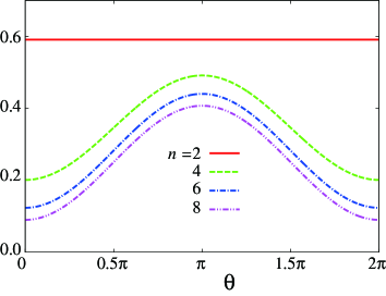
(a) ${n=}$ even

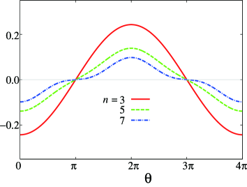
(b) ${n=}$ odd

Figure 2.1: ${\mathcal{O}(n,\theta)}$ for ${\Delta=1}$

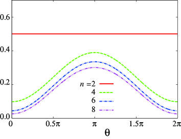
(a) ${n=}$ even

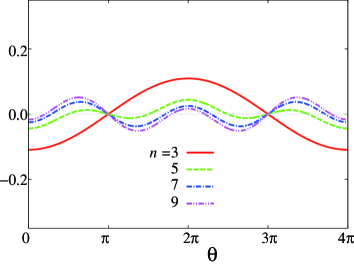
(b) ${n=}$ odd

Figure 2.2: ${\mathcal{O}(n,\theta)}$ for ${\Delta=1/2}$

From the figures one observes:

• For even ${n}$ (${\geq 4}$), ${\mathcal{O}(n,\theta)}$ is always positive with a period ${2\pi}$. It has a single maximum at ${\theta=\pi}$ and a minimum at ${\theta=0}$. Recall that ${\mathcal{O}(n,\pi)=(2{\rm i})^{n}\langle\prod_{k=1}^{n}S^{z}_{k}\rangle}$ and ${\mathcal{O}(n,0)=-4\langle S^{z}_{1}S^{z}_{n}\rangle}$.

• For odd ${n}$, ${\mathcal{O}(n,\theta)}$ has a rather complicated structure with a period ${4\pi}$. In this case, ${\mathcal{O}(n,\pi)}$ and ${\mathcal{O}(n,3\pi)}$ are always zero as they should be.

We give some exact values of ${\mathcal{O}(n,\pi)=(2{\rm i})^{n}\langle\prod_{k=1}^{n}S^{z}_{k}\rangle}$ for ${\Delta=1}$ and ${\Delta=1/2}$ in the following:

• ${\Delta=1}$

  $$\mathcal{O}(2,\pi) = -\frac{1}{3}+\frac{4}{3}\ln 2=0.5908629074132604\cdots$$

  $$\mathcal{O}(4,\pi) = \frac{1}{5}-\frac{16}{3}\ln 2+\frac{232}{15}\zeta(3)-\frac{32}{3}\ln 2\cdot\zeta(3)-\frac{21}{5}\zeta(3)^{2}$$

  $$-\frac{95}{6}\zeta(5)+\frac{70}{3}\ln 2\cdot\zeta(5)=0.4914453923615522\cdots$$

  $$\mathcal{O}(6,\pi) = 0.4403016697026268\cdots$$

  $$\mathcal{O}(8,\pi) = 0.4072424147596208\cdots$$ (2.13)

• ${\Delta=1/2}$

  $$\mathcal{O}(2,\pi) = \frac{1}{2}$$

  $$\mathcal{O}(4,\pi) = \frac{1595}{4096}=0.389404296875$$

  $$\mathcal{O}(6,\pi) = \frac{719423395}{2147483648}=0.3350076242350041\cdots$$

  $$\mathcal{O}(8,\pi) = \frac{346891287109196331}{1152921504606846976}=0.3008802296800668\cdots$$ (2.14)

One observes that ${\mathcal{O}(n,\pi)}$ for ${n}$=even decays very slowly as ${n}$ increases. Namely as mentioned in the introduction, for ${\Delta=1}$, the asymptotic decay ${\mathcal{O}(n,\pi)\sim n^{-1/4}}$ was given by Hida [7] and more generally

$$\mathcal{O}(n,\theta)\sim n^{-\frac{\theta^{2}}{4\pi^{2}}}$$ (2.15)

by Lou [8]. In the next section, we shall both generalize this asymptotic formula to the more general ${-1<\Delta<1}$ case and determine the amplitude by making use of field theory. Furthermore since the formula Eq. (2.15) does not explain the difference of the periodicity with respect to the parity of ${n}$, we shall consider some subleading terms more carefully. We remark that ${\rho(n,\theta)}$, Eq. (1.2), shares periodicity properties analogous to $\mathcal{O}(n,\theta)$. In fact it is easy to see that ${\rho(n,\theta)}$ is expanded as

$$\rho(n,\theta)=\sum_{j=1}^{n}P_{n,j}\cos\left[\left(\frac{n}{2}-j\right)\theta\right],$$ (2.16)

where the coefficients ${P_{n,j}}$ are the summation of the diagonal density matrix elements in the sector with ${j}$ down spins. Note that ${P_{n,j}=P_{n,n-j}}$. From Eq.(2.16), one can immediately find

$$\rho(n,\theta+2\pi)=(-1)^{n}\rho(n,\theta)$$ (2.17)

${\bullet}$ ${\Delta=0}$ case :

Let us comment on the string correlation functions for ${\Delta=0}$. In this case, a simple determinant formula for the string correlation function ${\rho(n,\theta)}$ exists (c.f. Ref.[43])

$$\rho(n,\theta)=\det\left[\left(\cos\frac{\theta}{2}\right)\delta_{j,k}+\left({\rm i}\sin\frac{\theta}{2}\right)M_{j,k}\right]_{j,k=1}^{n},\ \ \ \ M_{j,k}=\begin{cases}0&j-k:{\rm even}\\ \dfrac{2}{\pi}\dfrac{(-1)^{\frac{j-k+1}{2}}}{j-k}&j-k:{\rm odd}\end{cases}$$

(2.18)

Using this formula one can evaluate the exact numerical values up to the order of ${n\simeq 10000}$ easily, for example, by Mathematica on a standard PC. We give the exact values in Table 2.1 up to ${n=1000}$.

$n$	5	10	20	50	100	200	500	1000
$\rho(n,\pi/4)$	0.884857	0.866761	0.848076	0.824090	0.806421	0.789137	0.766860	0.750428
$\rho(n,\pi/2)$	0.605461	0.564975	0.516684	0.459997	0.421580	0.386481	0.344597	0.315979
$\rho(n,3\pi/4)$	0.289075	0.291125	0.234367	0.177503	0.144555	0.118072	0.0906455	0.0743400

Table 2.1: Exact values of ${\rho(n,\theta)}$ for ${\Delta=0}$

This determinant is also expressed as a Toeplitz determinant

$$\rho(n,\theta) = \mbox{e}^{{\rm i}n\theta/2}\det\left[\dfrac{1}{2\pi}\int_{0}^{2\pi}{\rm e}^{{\rm i}(j-k)q}\sigma(q){\rm d}q\right]_{j,k=1}^{n},\ \sigma(q)=\begin{cases}{\rm e}^{-{\rm i}\theta}&:0<q<\dfrac{\pi}{2}\\ 1&:\ \dfrac{\pi}{2}<q<\dfrac{3\pi}{2}\\ {\rm e}^{-{\rm i}\theta}&:\dfrac{3\pi}{2}<q<2\pi\\ \end{cases}$$

There are some mathematical results known on the asymptotic behaviours of Toeplitz determinants as ${n\to\infty}$. Assume ${\theta\neq 0,2\pi}$, then “the generating function” ${\sigma(q)}$ of the Toeplitz determinant has jump singularities at ${q=\pi/2}$ and ${q=3\pi/2}$. In such a case, we can invoke the (generalized) Fisher-Hartwig conjecture [44, 45], which brings about an asymptotic formula for ${0<\theta<2\pi}$ as

$$\rho(n,\theta) \simeq \rho_{\rm Asym}^{(0)}(n,\theta)+(-1)^{n}\rho_{\rm Asym}^{(1)}(n,\theta),$$

$$\rho_{\rm Asym}^{(k)}(n,\theta) = n^{-2(-\frac{\theta}{2\pi}+k)^{2}}4^{-(-\frac{\theta}{2\pi}+k)^{2}}\left[G(1+\frac{\theta}{2\pi}-k)G(1-\frac{\theta}{2\pi}+k)\right]^{2}.$$ (2.20)

Here ${G(z)}$ is the Barnes $G$-function defined by

$$G(z+1)=(2\pi)^{\frac{1}{2}z}\exp\left(-\frac{1}{2}z-\frac{1}{2}(\gamma+1)z^{2}\right)\prod_{k=1}^{\infty}\left\{\left(1+\frac{z}{k}\right)^{k}\exp\left(-z+\frac{z^{2}}{2k}\right)\right\}$$

where ${\gamma=0.5772156649\cdots}$ is the Euler-Mascheroni constant. Each term ${\rho_{\rm Asym}^{(k)}(n,\theta)}$ decays algebraically with the exponent ${-2\left(-\frac{\theta}{2\pi}+k\right)^{2}}$. Then the dominant term is ${\rho_{\rm Asym}^{(0)}(n,\theta)}$ for ${0<\theta<\pi}$, and ${(-1)^{n}\rho_{\rm Asym}^{(1)}(n,\theta)}$ for ${\pi<\theta<2\pi}$. We refer the reader also to Refs. [46, 47] for more information about the (generalized) Fisher-Hartwig conjectures.

$n$	5	10	20	50	100	200	500	1000
$\rho_{\rm Asym}(n,\pi/4)$	0.884970	0.866783	0.848081	0.824091	0.806421	0.789137	0.766860	0.750428
$\rho_{\rm Asym}(n,\pi/2)$	0.605720	0.565076	0.516705	0.460000	0.421581	0.386481	0.344597	0.315979
$\rho_{\rm Asym}(n,3\pi/4)$	0.289328	0.291316	0.234403	0.177507	0.144555	0.118072	0.0906455	0.0743400

Table 2.2: Numerical values obtained from the asymptotic formula ${\rho_{\rm Asym}(n,\theta)}$ for ${\Delta=0}$

Numerical values calculated from Eq. (2.20) are listed in Table 2.2. Good agreement is found with the data in Table 2.1. In this context, it is remarkable that they coincide within at least three digits even for small sizes as ${n=10}$. Finally let us note a further exact result for ${\rho(n,\pi)}$ at ${\Delta=0}$. Since ${\rho(2m-1,\pi)=0}$, we consider ${\rho(2m,\pi)}$, which is given more explicitly as

$$\rho(2m,\pi) = (-1)^{m}2^{2m}\left\langle\prod_{j=1}^{2m}S_{j}^{z}\right\rangle=(-1)^{m}{\rm det}\left[M_{j,k}\right]_{j,k=1}^{2m}$$ (2.21)

$$= \left(\frac{2}{\pi}\right)^{2m}\prod_{k=1}^{m}\prod_{j\neq k}^{m}\left(\frac{j-k}{j-k-1/2}\right)^{2}=\prod_{k=1}^{m}\frac{\Gamma^{4}(k)}{\Gamma^{2}(k-\frac{1}{2})\Gamma^{2}(k+\frac{1}{2})}$$

$$= \exp\left[-\frac{1}{2}\int_{0}^{\infty}\frac{{\rm d}t}{t}\frac{1-{\rm e}^{-mt}}{\cosh^{2}(t/4)}\right]$$

$$= c_{0}m^{-1/2}\exp\left[-\frac{1}{2}\int_{0}^{\infty}\frac{{\rm d}t}{t}{\rm e}^{-t}\tanh^{2}\left(\frac{t}{4m}\right)\right]$$

$$= c_{0}m^{-1/2}\left(1-\frac{1}{32}m^{-2}+\frac{17}{2048}m^{-4}-\frac{379}{65536}m^{-6}+\cdots\right),$$

where

$$c_{0} = {\rm exp}\left[\frac{1}{2}\int_{0}^{\infty}\frac{{\rm d}t}{t}\left({\rm e}^{-4t}-\frac{1}{\cosh^{2}t}\right)\right]=\left[G\left(\frac{1}{2}\right)G\left(\frac{3}{2}\right)\right]^{2}.$$

Here we have used an integral formula for the logarithm of the Euler gamma function,

$$\log\Gamma(z)=\int_{0}^{\infty}\left[(z-1)-\frac{1-{\rm e}^{(-z+1)t}}{1-{\rm e}^{-t}}\right]\frac{{\rm e}^{-t}}{t}{\rm d}t,\ \ \ \ \ \ (\Re(z)>0).$$ (2.22)

Thus we can obtain the asymptotic expansion to an arbitrary order in this case. Note that the leading term is consistent with the formula Eq. (2.20) with ${\theta=\pi}$.

3 Asymptotic behaviour of string correlation functions

In this section, we will discuss the asymptotic behaviour of the string correlation functions for the critical region ${-1<\Delta<1}$ (that is $\pi>\gamma>0$) by use of field theoretical arguments. Thus the aim is to find coefficients $D_{j}$ and exponents $\nu_{j}$ such that

$$\lim_{n\to\infty}\frac{\rho(n,\theta)-\sum_{j=1}^{m-1}D_{j}(\theta,\gamma)n^{-\nu_{j}(\theta,\gamma)}}{n^{-\nu_{m}(\theta,\gamma)}}=:D_{m}(\theta,\gamma)\;\,\text{(finite)},\;\,m=1,2,\ldots.$$ (3.1)

The exponents are increasing with $j$, i.e. $\nu_{j}<\nu_{j+1}$. The amplitudes and exponents depend on the parameters $\theta,\gamma$ of the model and of the function $\rho$. Instead of Eq. (3.1), we use the shorthand notation

$$\rho(n,\theta)\sim\sum_{j}D_{j}(\theta,\gamma)n^{-\nu_{j}(\theta,\gamma)}.$$

The important point to remember is that the asymptotic expansion is defined in the limit $n\to\infty$.

We first present the results obtained so far within the field-theoretical framework and give details of the derivation in the following section.

3.1 Results

We find the following asymptotic expansion of the string correlation function for $0<\theta\leq\pi$:

$$\rho(n,\theta) \equiv \left\langle\exp\left[{\rm i}\theta\sum_{k=1}^{n}S_{k}^{z}\right]\right\rangle$$

$$\sim D(\theta,\gamma)n^{-\nu_{1}(\theta,\gamma)}\left(1+\mathcal{O}\left(n^{-\delta(\gamma)}\right)\right)$$

$$+(-1)^{n}D(2\pi-\theta,\gamma)n^{-\nu_{1}(2\pi-\theta,\gamma)}\left(1+\mathcal{O}\left(n^{-\delta(\gamma)}\right)\right)$$

$$+\mathcal{O}\left(n^{-\nu_{1}(\theta,\gamma)-2},(-1)^{n}n^{-\nu_{1}(2\pi+\theta,\gamma)},(-1)^{n}n^{-\nu_{1}(2\pi+\theta,\gamma)-2},(-1)^{n}n^{-\nu_{1}(2\pi-\theta,\gamma)-2}\right)\,,$$

with

$$\nu_{1}(\theta,\gamma) = \frac{\theta^{2}}{4\pi^{2}}\,\frac{\pi}{\pi-\gamma}$$

$$\delta(\gamma) = 4\frac{\pi}{\pi-\gamma}-4$$

$$D(\theta,\gamma) = \left[\frac{\Gamma\left(\frac{\eta}{2-2\eta}\right)}{2\sqrt{\pi}\Gamma\left(\frac{1}{2-2\eta}\right)}\right]^{\theta^{2}/(4\eta\pi^{2})}$$

$$\times\exp\left[-\int_{0}^{\infty}\left(\frac{\sinh^{2}\frac{\theta}{2\pi}t}{\sinh t\,\cosh(1-\eta)t\,\sinh\eta t}-\frac{\theta^{2}\mbox{e}^{-2t}}{4\eta\pi^{2}}\right)\frac{\mbox{d}t}{t}\right]$$

$$= \left[\frac{\Gamma\left(\frac{\pi R^{2}}{1-2\pi R^{2}}\right)}{2\sqrt{\pi}\Gamma\left(\frac{1}{2-4\pi R^{2}}\right)}\right]^{(\theta/(2\pi R))^{2}/(2\pi)}$$

$$\times\exp\left[-\int_{0}^{\infty}\left(\frac{\sinh^{2}\frac{\theta}{2\pi}t}{\sinh t\,\cosh(1-2\pi R^{2})t\,\sinh 2\pi R^{2}t}-\left(\frac{\theta}{2\pi R}\right)^{2}\frac{\mbox{e}^{-2t}}{2\pi}\right)\frac{\mbox{d}t}{t}\right]$$

In Eq. (3.1), Lukyanov’s notation is used with $\eta=\frac{\pi-\gamma}{\pi}$, whereas in Eq. (LABEL:coeffr), the anisotropy is written in terms of the compactification radius $R$ with $2\pi R^{2}=\eta$.

Since $\rho(n,\theta)=\rho(n,-\theta)$, the result (3.1) is readily extended to the domain $-\pi\leq\theta<0$. Thus $\rho(n,\theta)$ is known in the fundamental domain $-\pi\leq\theta\leq\pi$ (note ${\rho(n,\theta=0)=1}$, trivially). The periodicity Eq. (2.17) then yields $\rho$ for all values of $\theta$.

We note the following limiting values of the coefficient $D(\theta,\gamma)$:

• $D(\theta=2\pi\eta,\gamma)=2(1-\eta)^{2}A$, where $A$ is the coefficient of the leading term in an asymptotic expansion of the uniform part of $\langle\sigma^{x}_{1}\sigma^{x}_{n}\rangle$, namely: $\langle\sigma^{x}_{1}\sigma^{x}_{n}\rangle_{u}\sim\frac{A}{n^{\eta}}$, [32]. Then, as ${\nu_{1}(\theta=2\pi\eta,\gamma)=\eta}$, we have the asymptotic equality (note that $1-\eta=\gamma/\pi$) for $\pi/2\leq\gamma<\pi$

  $$\rho(n,2\pi\eta)\sim 2\left(\frac{\gamma}{\pi}\right)^{2}\langle\sigma^{x}_{1}\sigma^{x}_{n}\rangle_{u},\ \ \ \ \pi/2\leq\gamma<\pi$$ (3.5)

  for the leading order of the uniform part (in order to facilitate comparison with Lukyanov’s results, we use the Pauli-matrices $\sigma^{\nu}=2S^{\nu}$). This is checked immediately at the free fermion point $\Delta=0$ from Eq. (2.21).

• $D(0,\gamma)=1$, whereas

  $$\lim_{\theta\to 0}D(2\pi-\theta,\gamma)\frac{16}{\theta^{2}} = \frac{A_{z}}{2}$$

  $$\equiv \frac{4}{\pi^{2}}\left[\frac{\Gamma\left(\frac{\eta}{2-2\eta}\right)}{2\sqrt{\pi}\Gamma\left(\frac{1}{2-2\eta}\right)}\right]^{1/\eta}$$

  $$\times\exp\left[\int_{0}^{\infty}\left(\frac{\sinh((2\eta-1)t)}{\sinh(\eta t)\cosh((1-\eta)t)}-\frac{2\eta-1}{\eta}\mbox{e}^{-2t}\right)\frac{\mbox{d}t}{t}\right]$$

  . (3.6)

  The last equation is proved in Appendix B. Following Lukyanov’s notation [32], $A_{z}$ denotes the coefficient of the leading contribution in the alternating part $\langle\sigma_{1}^{z}\sigma_{n}^{z}\rangle_{a}$ of the $\sigma^{z}$-$\sigma^{z}$-correlation function, namely

  $$\langle\sigma^{z}_{1}\sigma_{n}^{z}\rangle_{a}\sim\frac{(-1)^{n-1}A_{z}}{n^{1/\eta}}.$$ (3.7)

In order to obtain the asymptotics of the generalized string correlation function, we first express it in terms of $\rho(n,\theta)$ according to Eq. (2.12). Then, using the above results, the asymptotic behavior of $\mathcal{O}(n,\theta)$ is obtained for ${0<\theta\leq\pi}$:

$$\mathcal{O}(n,\theta)\equiv-4\left\langle S_{1}^{z}\exp\left[{\rm i}\theta\sum_{k=2}^{n-1}S_{k}^{z}\right]S_{n}^{z}\right\rangle$$

$$\sim D(\theta,\gamma)n^{-\nu_{1}(\theta,\gamma)}\left[\tan^{2}\frac{\theta}{4}-\frac{\cos\frac{\theta}{2}}{\cos^{2}\frac{\theta}{4}}\,\frac{\nu_{1}(\theta,\gamma)}{n}+\frac{\cos\frac{\theta}{2}(2\cos\frac{\theta}{2}-1)}{\sin^{2}\frac{\theta}{2}}\frac{\nu_{1}(\theta,\gamma)(\nu_{1}(\theta,\gamma)+1)}{n^{2}}+\cdots\right]$$

$$+(-1)^{n}D(2\pi-\theta,\gamma)n^{-\nu_{1}(2\pi-\theta,\gamma)}$$

$$\times\Bigg{[}\cot^{2}\frac{\theta}{4}+\frac{\cos\frac{\theta}{2}}{\sin^{2}\frac{\theta}{4}}\,\frac{\nu_{1}(2\pi-\theta,\gamma)}{n}+\frac{\cos\frac{\theta}{2}(2\cos\frac{\theta}{2}+1)}{\sin^{2}\frac{\theta}{2}}\frac{\nu_{1}(2\pi-\theta,\gamma)(\nu_{1}(2\pi-\theta,\gamma)+1)}{n^{2}}+\cdots\Bigg{]}$$

Let us consider the limit $\theta\to 0$ of the asymptotic formula Eq.(LABEL:oasym). The first two terms of the uniform part in (LABEL:oasym) vanish in this limit and the third term gives

$$\lim_{\theta\to 0}D(\theta,\gamma)n^{-\nu_{1}(\theta,\gamma)}\left[\frac{\cos\frac{\theta}{2}(2\cos\frac{\theta}{2}-1)}{\sin^{2}\frac{\theta}{2}}\frac{\nu_{1}(\theta,\gamma)(\nu_{1}(\theta,\gamma)+1)}{n^{2}}\right]=\frac{1}{\pi(\pi-\gamma)n^{2}}=\frac{1}{\pi^{2}\eta n^{2}}$$ (3.9)

Because of the relation Eq. (3.6), the leading alternating part yields

$$\lim_{\theta\to 0}(-1)^{n}D(2\pi-\theta,\gamma)n^{-\nu_{1}(2\pi-\theta,\gamma)}\cot^{2}\frac{\theta}{4}=\frac{(-1)^{n}A_{z}}{2n^{1/\eta}}$$ (3.10)

In order to get the correct leading alternating term in the limit $\theta\to 0$, we should also consider the leading alternating part for ${-\pi\leq\theta<0}$, which reads

$$(-1)^{n}D(2\pi+\theta,\gamma)n^{-\nu_{1}(2\pi+\theta,\gamma)}\left[\cot^{2}\frac{\theta}{4}+\frac{\cos\frac{\theta}{2}}{\sin^{2}\frac{\theta}{4}}\,\frac{\nu_{1}(2\pi+\theta,\gamma)}{n}+\cdots\right]$$ (3.11)

in addition to (LABEL:oasym). Then we have similarly to Eq. (3.10)

$$\lim_{\theta\to 0}(-1)^{n}D(2\pi+\theta,\gamma)n^{-\nu_{1}(2\pi+\theta,\gamma)}\cot^{2}\frac{\theta}{4}=\frac{(-1)^{n}A_{z}}{2n^{1/\eta}}$$ (3.12)

in the limit ${\theta\to 0}$. Collecting the terms (3.9), (3.10) and (3.12) yields

$$\lim_{\theta\to 0}\mathcal{O}(n,\theta)\sim\frac{(-1)^{n}A_{z}}{n^{1/\eta}}+\frac{1}{\pi^{2}\eta n^{2}}.$$ (3.13)

Eq. (3.13) coincides with the leading asymptotic behaviour of two-point correlation function ${-4\left\langle S_{1}^{z}S_{n}^{z}\right\rangle=-\left\langle\sigma_{1}^{z}\sigma_{n}^{z}\right\rangle}$.

3.2 Derivation

3.2.1 The string correlation function $\rho(n,\theta)$

An effective field theory describing the low-energy-excitations of the XXZ-chain in the critical regime $0<\gamma<\pi$ has been derived by Lukyanov [31]. At zero magnetic field, the corresponding Hamiltonian density $\mathcal{H}$ reads

$$\mathcal{H} = \frac{v}{2}\left(\Pi(x)^{2}+(\partial_{x}\varphi(x))^{2}\right)+\varepsilon^{1/(\pi R^{2})-2}\lambda\cos\frac{2\varphi(x)}{R}$$ (3.14)

$$+\varepsilon^{2}\left[\lambda_{+}J_{L}^{2}(x)J_{R}^{2}(x)+\lambda_{-}\left[J_{L}^{4}(x)+J_{R}^{4}(x)\right]\right]+\ldots,$$

where the dots denote terms with scaling dimensions higher than those given explicitly. The dimensionless constants $v,\lambda,\lambda_{\pm}$ are known exactly from Bethe Ansatz [31]. The lattice constant $\varepsilon$ has the dimension of a length, whereas the dimension of $\mathcal{H}$ is 1/length². Above, $\mathcal{H}$ is the sum of a Gaussian model and irrelevant operators, the latter with scaling dimensions $1/(\pi R^{2})$ and $4$. The Hamiltonian is written in terms of the bosonic field $\varphi$ and its momentum $\Pi$, where $\left[\varphi(x),\Pi(y)\right]={\rm i}\delta(x-y)$. The left- and right current operators are then defined as $J_{L,R}(x)=\frac{\mp 1}{\sqrt{4\pi}}\left(\Pi(x)\pm\varphi(x)\right)$.

Within the same approach, the effective $S^{z}$-operator reads

$$S^{z}_{j}\equiv S^{z}(x) \sim \frac{\varepsilon}{2\pi R}\partial_{x}\varphi(x)+\sum_{m=0}^{\infty}(-1)^{m}\varepsilon^{(2m+1)^{2}/(4\pi R^{2})}C_{m}\cos\left(\frac{2m+1}{R}\varphi(x)\right)$$ (3.15)

$$+\mbox{descendants}\,,$$

where $x=\varepsilon j$. The constants $C_{m}$ have been determined in [32]. We do not write down the descendant fields here explicitly, but only note that if a primary field has scaling dimension $\Delta$, then the descendant fields have scaling dimension $\Delta+\ell$, where $\ell$ is a certain positive integer.

To arrive at an asymptotic expression for $\rho(n,\theta)$, we first apply the Euler-MacLaurin formula to the sum in the exponent:

$$\sum_{k=1}^{n}S_{k}^{z} = \varepsilon^{-1}\int_{0}^{x}S^{z}(x^{\prime})\mbox{d}x^{\prime}-\frac{1}{2}\left[S^{z}(0)-S^{z}(x)\right]+\mathcal{O}(\partial^{\mu}_{x}S^{z})$$ (3.16)

$$= \frac{1}{2\pi R}\left(\varphi(x)-\varphi(0)\right)+\mathcal{O}(\varepsilon^{(2m+1)^{2}/(4\pi R^{2})+\mu},\varepsilon^{\mu}),$$

($\mu\geq 1$ integer) from which one concludes that the only cutoff-independent contribution in the integral stems from the first term in the last equation. We expand the exponent with respect to $\varepsilon$ and arrive at

$$\rho(n,\theta)\sim\left\langle\exp\left[{\rm i}\frac{\theta}{2\pi R}(\varphi(x)-\varphi(0))\right]\left(1+\mathcal{O}(\varepsilon^{2k\left[(2m+1)^{2}/(4\pi R^{2})+\mu\right]},\varepsilon^{2k\mu})\right)\right\rangle$$ (3.17)

where the positive integer $k$ originates in the expansion of the exponential function. From this we conclude that the leading exponent of the uniform part is $\nu_{1}(\theta,\gamma)$, and the leading Euler-MacLaurin corrections to this have exponents $\nu_{1}(\theta,\gamma)+2,\nu_{1}(\theta,\gamma)+1/(2\pi R^{2})$.

Thus in order to determine the amplitude of the leading term, we have to calculate
$\left\langle\exp\left[{\rm i}\frac{\theta}{2\pi R}(\varphi(x)-\varphi(0))\right]\right\rangle$. In the field-theoretical setting of massless Bose fields considered here, this quantity is defined only up to a multiplicative constant $\Lambda$ with dimension 1/length [32]. It has become custom to choose it such that (“CFT normalization condition”)

$$\Lambda^{\alpha^{2}/(2\pi)}\langle\exp\left[{\rm i}\alpha(\varphi(x)-\varphi(0))\right]\rangle=|x|^{-\alpha^{2}/(2\pi)}.$$ (3.18)

This means that we have to introduce a constant $D(\theta,\gamma)$ as follows:

$$\rho(n,\theta)\sim D(\theta,\gamma)\left\langle\exp\left[{\rm i}\frac{\theta}{2\pi R}(\varphi(x)-\varphi(0))\right]\right\rangle=\frac{D(\theta,\gamma)}{n^{(\theta/2\pi R)^{2}/(2\pi)}}$$ (3.19)

for the leading decay of the uniform part. Because of the symmetry $\rho(n,-\theta)=\rho(n,\theta)$, this result is valid for $-\pi\leq\theta\leq\pi$. Let us defer the calculation of the coefficient $D$ to the next paragraph and first determine the leading exponent of the alternating part. This is obtained directly by exploiting the periodicity Eq. (2.17). Together with Eq. (3.19), it implies that

$$\rho(n,\pi\leq\theta\leq 3\pi) \sim D(\theta-2\pi,\gamma)n^{-\nu_{1}(\theta-2\pi,\gamma)}$$ (3.20)

$$\rho(n,-3\pi\leq\theta\leq-\pi) \sim D(\theta+2\pi,\gamma)n^{-\nu_{1}(\theta+2\pi,\gamma)}.$$ (3.21)

The exponents are expected to depend continuously on the parameters $\theta,\gamma$. Thus for $0\leq\theta\leq\pi$ ($-\pi\leq\theta<0$), Eq. (3.20) (Eq. (3.21)) yields the leading contribution to the alternating part, which is next-leading with respect to the leading decay given in Eq. (3.19).

What are the exponents of the next-leading contributions? In Eq. (3.19) we have tacitly assumed that the expectation value is taken with respect to the unperturbed Gaussian part of the Hamiltonian (3.14). However, there are additional contributions in Eq. (3.14), with scaling dimensions $\Delta=1/(\pi R^{2}),4$. As argued in [34], they lead to exponents $\nu_{1}(\theta,\gamma)+k(\Delta-2)$ in $\left\langle\exp\left[{\rm i}\frac{\theta}{2\pi R}(\varphi(x)-\varphi(0))\right]\right\rangle$, where the integer $k$ denotes the order of the perturbational expansion. Since there is no contribution of the $\cos$-operator for $k=1$, the next-leading exponent stemming from this contribution is $\nu_{2}(\theta,\gamma)=\nu_{1}(\theta,\gamma)+\delta(\gamma)$ with $\delta(\gamma)=4\pi/(\pi-\gamma)-4$. On the other hand, the first-order contribution of the $\lambda_{\pm}$-operators yields an exponent $\nu_{1}(\theta,\gamma)+2$. This latter one is always larger than $\nu_{1}(\theta,\gamma),\nu_{1}(\theta-2\pi,\gamma)$ (for $0<\theta<\pi$) and we discard it here. Thus $\nu_{2}(\theta,\gamma)$ yields the next-leading exponent in the uniform part. According to the periodicity argument, the next-leading exponent in the alternating part for $0<\theta<\pi$ is then $\nu_{2}(\theta-2\pi,\gamma)$.

We now focus on the coefficient $D(\theta,\gamma)$. The result given in Eq. (3.1) is a conjecture based on the work [33]. The following tests of this conjecture have been performed:

• For $\gamma=\pi/2$, one can show that $D(\theta,\pi/2)$ reduces to (2.20), namely

  $$D(\theta,\pi/2) = 4^{-\frac{\theta^{2}}{4\pi^{2}}}\left[G\left(1+\frac{\theta}{2\pi}\right)G\left(1-\frac{\theta}{2\pi}\right)\right]^{2}.$$ (3.22)

  This equality can be checked by means of an integral representation of the Barnes $G$-function (see Appendix C).

• Numerical comparisons for $\Delta=1/2$ between the exact data from the Bethe Ansatz (for $n=9$) and the asymptotic results (3.1),(LABEL:oasym) have been performed for $\theta=\pi/4,\pi/2,3\pi/4,\pi$. In all cases, very good agreement is found. Similarly, we compared with the data obtained by the numerical diagonalization up to a system size of ${N=28}$ lattice sites for general ${\Delta}$ (see Appendix A).

Our conjecture for $D$ is based on arguments similar to the conjecture for the coefficient of the leading decay of $\langle\sigma^{x}_{1}\sigma^{x}_{n}\rangle$, cf. [32], [33]. In [33], the expectation value of $\langle\exp\left[{\rm i}\alpha\vartheta\right]\rangle$ in a massive Sine-Gordon model with an operator $\cos(\beta\vartheta)$ is determined,

$$\langle\exp\left[{\rm i}\alpha\vartheta\right]\rangle=(\varepsilon m)^{\alpha^{2}/(4\pi)}N(\alpha,\beta),$$ (3.23)

where $m$ is the particle mass associated with the field $\vartheta$. Since in that problem, $\sigma^{x}\sim\mbox{e}^{{\rm i}2\pi R\vartheta}$ with an a priori unknown amplitude, calculating the amplitude of the leading decay of $\langle\sigma^{x}_{1}\sigma^{x}_{n}\rangle$ with respect to a Sine-Gordon model with an operator $\cos(\beta\vartheta)$ is very similar to our problem of determining $D$.

An explicit value for $N(\alpha,\beta)$ in Eq. (3.23) is conjectured and confirmed explicitly in certain limiting cases in [33]. The authors then calculate $\langle\sigma_{1}^{x}\sigma_{n}^{x}\rangle\sim A(\eta)N(1/\eta,2/R)n^{-\eta}$ by making use of the fact that this correlation function is known explicitly for the massive XYZ-model close to the critical XXZ-point, namely $\langle\sigma_{1}^{x}\sigma_{n}^{x}\rangle_{m}\sim A_{m}(\varepsilon m)^{-\eta}$ with a known coefficient $A_{m}$. This allows for the deduction of $A(\eta)$.

In our case, the field $\varphi$ is related to $\vartheta$ by $\partial_{t}\varphi=\partial_{x}\vartheta$. However, the problem of calculating $D$ is completely analogous to the calculation of $A(\eta)$ sketched above, with a Sine-Gordon-term $\cos(2\varphi/R)$ in the Hamiltonian. The only unknown is the string function $\rho_{m}(\theta)$ in the massive XYZ-regime. We know that

$$\rho_{m}(\theta)=C_{m}(R)(\varepsilon m)^{(\theta/(2\pi R))^{2}/(2\pi)}$$ (3.24)

with an unknown constant $C_{m}$ depending on $R$. Note that in the massive regime, we cannot relate $2/R$ to $\gamma$, but rather take it as the constant in the Sine-Gordon-term $\cos(2\varphi/R)$. On the other hand, the results in [33] tell us that

$$\rho_{m}(\theta)=D\,N(\theta/(2\pi R),2/R)(\varepsilon m)^{(\theta/(2\pi R))^{2}/(2\pi)}$$ (3.25)

with a known coefficient $N(\theta/(2\pi R),2/R)$. By comparing Eq. (3.25) with Eq. (3.24), one obtains $D$ in terms of $\theta$, $R$ and the unknown $C_{m}(R)$. We find that $C_{m}(R)=2(1-\eta)^{2}=2(1-2\pi R^{2})^{2}$ yields excellent agreement with the numerical data as described above. This results in the coefficient $D(\theta,\gamma)$ as given in Eqs. (3.1), (LABEL:coeffr).

We finally comment on the isotropic case, $\gamma=0$. Here, $\nu_{1}(\theta,\gamma=0)=\theta^{2}/(4\pi^{2})$, in agreement with the result of [8]. However, we expect that a logarithmic dependence of the amplitude on the distance occurs, similarly to what happens for the two-point functions [30, 31, 32]. We leave the study of this case as a project for future research.

3.2.2 The generalized string correlation function $\mathcal{O}(n,\theta)$

From Eq. (2.12), the asymptotics of $\mathcal{O}(n,\theta)$ is obtained once the asymptotics of $\rho(n,\theta)$ is known. It is nevertheless instructive to perform a consistency check of this result by calculating the asymptotics of $\mathcal{O}$ directly by using field-theoretical arguments.

Therefore, one might be tempted to take the asymptotic expansion of $S^{z}(x)$, Eq. (3.15), and insert it into Eq. (1.1). However, in such a calculation the leading terms given in Eq. (3.1) would be absent. We are thus lead to use the following asymptotic expansion for the $S^{z}$-operators at sites $1$ and $n$ involved in $\mathcal{O}(n,\theta\neq 0)$:

$$S^{z}(x) \sim s_{0}+\frac{\varepsilon}{2\pi R}\partial_{x}\varphi(x)$$ (3.26)

$$+\sum_{m=0}^{\infty}(-1)^{j}\varepsilon^{(2m+1)^{2}/(4\pi R^{2})}C_{m}\cos\left(\frac{2m+1}{R}\varphi(x)\right)+\mbox{descendants }\,,$$

with $x=\varepsilon j$. The asymptotic expansion starts with a finite constant $s_{0}$. For the asymptotics of the phase factor in $\mathcal{O}(n,\theta)$, we still use Eq. (3.15). Carrying out the same calculations as above, one finds $s_{0}^{2}=\tan^{2}(\theta/4)$, which vanishes for $\theta=0$. The intriguing point is that we have to modify the asymptotic expansion for the spins at sites 1 and $n$ in $\mathcal{O}(n,\theta)$ without modifying the Hamiltonian. Namely, it looks as if in the asymptotic limit, the phase operator in $\mathcal{O}(n,\theta)$ acts as a local field on the edge spins.

4 Conclusion and outlook

We evaluated the string correlation functions $\rho(n,\theta)$ and $\mathcal{O}(n,\theta)$ for the critical anisotropic spin-1/2 chain. For small $n$, exact results were obtained from the Bethe Ansatz, whereas in the asymptotic limit, both the amplitudes and the exponents of the leading decay could be determined from field theory. The field-theoretical results agree well with the Bethe Ansatz data. Especially, for $\Delta=0$, the asymptotics could be confirmed directly from the Bethe Ansatz results.

Most interestingly, the leading decay of the two-point $xx$-correlation function was recovered, Eq. (3.5). Whether this result has a physical background has to be clarified. As far as the limit $\theta\to 0$ in $\mathcal{O}(n,\theta)$ is concerned, we have recovered the expected result Eq. (3.13). However, the rather heuristic expansion (3.26) in the field-theory for $\theta\neq 0$ deserves further investigations in the future.

Appendix A Numerical values of string correlation functions

For ${\Delta=1}$ and ${1/2}$, the string correlation functions ${\rho(n,\theta)}$ and ${\mathcal{O}(n,\theta)}$ can be evaluated analytically up to ${n=8}$ and ${n=9}$, respectively. Here firstly, we list their precise numerical values for ${\theta=\pi/4,\pi/2,3\pi/4,\pi}$ up to ${n=8}$, based on these analytical expressions (see Table A.1 and Table A.2). Note that ${\rho(1,\theta)=\cos\frac{\theta}{2}}$ irrespective of ${\Delta}$ and therefore we have

$$\rho\left(1,\frac{\pi}{4}\right) = \cos\frac{\pi}{8}=0.923880,\ \ \ \ \rho\left(1,\frac{\pi}{2}\right)=\cos\frac{\pi}{4}=0.707107,$$

$$\rho\left(1,\frac{3\pi}{4}\right) = \cos\frac{3\pi}{8}=0.382683,\ \ \ \ \rho\left(1,\pi\right)=0.$$

Note also that ${\mathcal{O}(2,\theta)=-4\langle S_{1}^{z}S_{2}^{z}\rangle}$ irrespective of ${\theta}$ by its definition.

$n$	2	3	4	5	6	7	8
$\rho(n,\pi/4)$	0.940083	0.915627	0.925111	0.910171	0.917092	0.90616	0.911707
$\rho(n,\pi/2)$	0.795431	0.685542	0.744898	0.671293	0.718266	0.66085	0.70065
$\rho(n,3\pi/4)$	0.65078	0.362761	0.565509	0.349604	0.521325	0.339972	0.492564
$\rho(n,\pi)$	0.590863	0	0.491445	0	0.440302	0	0.407242
$\mathcal{O}(n,\pi/4)$	0.590863	-0.224243	0.24353	-0.120692	0.170343	-0.0786391	0.137344
$\mathcal{O}(n,\pi/2)$	0.590863	-0.171628	0.34622	-0.0787594	0.282725	-0.038569	0.2504
$\mathcal{O}(n,3\pi/4)$	0.590863	-0.0928846	0.44891	-0.0352563	0.394313	-0.00917944	0.361674

Table A.1: Exact values of string correlation functions for ${\Delta=1}$

$n$	2	3	4	5	6	7	8
$\rho(n,\pi/4)$	0.926777	0.909081	0.909299	0.900034	0.899811	0.893662	0.893337
$\rho(n,\pi/2)$	0.75	0.668437	0.692139	0.644847	0.661899	0.628299	0.641883
$\rho(n,3\pi/4)$	0.573223	0.346957	0.477542	0.32521	0.429591	0.310018	0.398987
$\rho(n,\pi)$	0.5	0.	0.389404	0.	0.335008	0.	0.30088
$\mathcal{O}(n,\pi/4)$	0.5	-0.101049	0.14059	-0.0285505	0.0880858	-0.00509166	0.0689805
$\mathcal{O}(n,\pi/2)$	0.5	-0.0773398	0.243652	0.000467493	0.192033	0.0293118	0.168568
$\mathcal{O}(n,3\pi/4)$	0.5	-0.041856	0.346715	0.012332	0.29362	0.033798	0.263161

Table A.2: Exact values of string correlation functions for ${\Delta=1/2}$

For ${\Delta=1/2}$ let us compare the results above with the numerical value of the asymptotic formulae Eq. (3.1) and Eq. (LABEL:oasym) with ${\gamma=\pi/3}$ in Table A.3.

$n$	2	3	4	5	6	7	8
$\rho_{\rm Asym}(n,\pi/4)$	0.926694	0.909865	0.909106	0.900388	0.899692	0.893859	0.893259
$\rho_{\rm Asym}(n,\pi/2)$	0.751733	0.669839	0.692208	0.645454	0.661862	0.628622	0.641843
$\rho_{\rm Asym}(n,3\pi/4)$	0.577912	0.348016	0.478151	0.325667	0.429729	0.310258	0.399020
$\rho_{\rm Asym}(n,\pi)$	0.506119	0	0.390271	0	0.335222	0	0.300940
$\mathcal{O}_{\rm Asym}(n,\pi/4)$	0.306262	-0.0812361	0.116753	-0.0204905	0.0793274	-0.000774240	0.0644446
$\mathcal{O}_{\rm Asym}(n,\pi/2)$	0.402260	-0.0722680	0.233892	0.00275605	0.1888360	0.0305388	0.167037
$\mathcal{O}_{\rm Asym}(n,3\pi/4)$	0.477679	-0.0413030	0.344917	0.0128694	0.293024	0.0341302	0.262857

Table A.3: Asymptotic formulas of string correlation functions for ${\Delta=1/2}$

We find the exact values and the asymptotic formulas are in good agreement especially for ${\rho(n,\theta)}$. The deviation is somewhat larger for ${\mathcal{O}(n,\theta)}$, for which we probably need higher order corrections to the asymptotic formulas to achieve better agreement.

To confirm our asymptotic formula further, we have calculated ${\rho(n,\theta)}$ numerically for several values of ${\Delta(=\pm 0.3,\pm 0.7,-0.5)}$ by means of the exact diagonalization for finite systems ${N=20\sim 28}$. Then we have applied an extrapolation according to $c_{0}+c_{1}/N^{2}+c_{2}/N^{3}+c_{3}/N^{4}+c_{4}/N^{5}$ and estimated ${\rho_{\rm Num}(n,\theta)}$ in the thermodynamic limit. These values are compared with our asymptotic formula ${\rho_{\rm Asym}(n,\theta)}$ in Tables A.4-A.8. We conclude that our asymptotic formula gives fairly precise values for all ranges of ${\Delta}$ in the critical region.

$n$	2	3	4	5	6	7	8
$\rho_{\rm Num}(n,\pi/4)$	0.921405	0.905433	0.902971	0.894779	0.892836	0.887437	0.885867
$\rho_{\rm Asym}(n,\pi/4)$	0.921707	0.905979	0.902974	0.894999	0.892828	0.887552	0.885852
$\rho_{\rm Num}(n,\pi/2)$	0.731659	0.658904	0.671538	0.631168	0.640067	0.612185	0.619215
$\rho_{\rm Asym}(n,\pi/2)$	0.734432	0.659884	0.672036	0.631562	0.640252	0.612384	0.619276
$\rho_{\rm Num}(n,3\pi/4)$	0.541914	0.338150	0.444087	0.312623	0.395710	0.295270	0.365120
$\rho_{\rm Asym}(n,3\pi/4)$	0.548200	0.338908	0.445270	0.312938	0.396134	0.295431	0.365265

Table A.4: Numerical values of ${\rho(n,\theta)}$ for ${\Delta=0.3}$

$n$	2	3	4	5	6	7	8
$\rho_{\rm Num}(n,\pi/4)$	0.932056	0.912068	0.915471	0.904519	0.906536	0.899088	0.900492
$\rho_{\rm Asym}(n,\pi/4)$	0.931684	0.913012	0.915038	0.905020	0.906242	0.899399	0.900275
$\rho_{\rm Num}(n,\pi/2)$	0.768025	0.676242	0.712563	0.656541	0.683506	0.642401	0.664320
$\rho_{\rm Asym}(n,\pi/2)$	0.768824	0.677927	0.712076	0.657389	0.683096	0.642903	0.663983
$\rho_{\rm Num}(n,3\pi/4)$	0.603994	0.354168	0.511302	0.335990	0.464170	0.322975	0.433890
$\rho_{\rm Asym}(n,3\pi/4)$	0.607173	0.355419	0.511188	0.336608	0.463845	0.323332	0.433544

Table A.5: Numerical values of ${\rho(n,\theta)}$ for ${\Delta=0.7}$

$n$	2	3	4	5	6	7	8
$\rho_{\rm Num}(n,\pi/4)$	0.903373	0.887893	0.878937	0.870856	0.865109	0.859693	0.855477
$\rho_{\rm Asym}(n,\pi/4)$	0.903927	0.887947	0.879042	0.870896	0.865149	0.859714	0.855487
$\rho_{\rm Num}(n,\pi/2)$	0.670096	0.61307	0.597811	0.569629	0.559974	0.541915	0.534903
$\rho_{\rm Asym}(n,\pi/2)$	0.674020	0.613330	0.598582	0.569822	0.560266	0.542024	0.535013
$\rho_{\rm Num}(n,3\pi/4)$	0.436818	0.295804	0.332446	0.256666	0.283712	0.232404	0.253962
$\rho_{\rm Asym}(n,3\pi/4)$	0.446622	0.296198	0.334401	0.256936	0.284437	0.232560	0.254249

Table A.6: Numerical values of ${\rho(n,\theta)}$ for ${\Delta=-0.3}$

$n$	2	3	4	5	6	7	8
$\rho_{\rm Num}(n,\pi/4)$	0.895942	0.877985	0.866417	0.857132	0.849944	0.843718	0.838522
$\rho_{\rm Asym}(n,\pi/4)$	0.895477	0.877611	0.866290	0.857039	0.849893	0.843674	0.838481
$\rho_{\rm Num}(n,\pi/2)$	0.644723	0.587178	0.562522	0.535287	0.520367	0.503241	0.492689
$\rho_{\rm Asym}(n,\pi/2)$	0.646724	0.586707	0.562879	0.535292	0.520512	0.503266	0.492719
$\rho_{\rm Num}(n,3\pi/4)$	0.393503	0.271884	0.284932	0.226344	0.236472	0.199498	0.207607
$\rho_{\rm Asym}(n,3\pi/4)$	0.402915	0.271927	0.286782	0.226578	0.237163	0.199648	0.207867

Table A.7: Numerical values of ${\rho(n,\theta)}$ for ${\Delta=-0.5}$

$n$	2	3	4	5	6	7	8
$\rho_{\rm Num}(n,\pi/4)$	0.886810	0.863491	0.847596	0.835540	0.825990	0.818029	0.811263
$\rho_{\rm Asym}(n,\pi/4)$	0.883755	0.861533	0.846496	0.834864	0.825552	0.817718	0.811018
$\rho_{\rm Num}(n,\pi/2)$	0.613546	0.549304	0.512895	0.483364	0.462734	0.444631	0.430668
$\rho_{\rm Asym}(n,\pi/2)$	0.610618	0.545990	0.511485	0.482427	0.462241	0.444263	0.430380
$\rho_{\rm Num}(n,3\pi/4)$	0.340281	0.236892	0.225198	0.182532	0.177268	0.153088	0.150087
$\rho_{\rm Asym}(n,3\pi/4)$	0.348075	0.235495	0.226127	0.182395	0.177655	0.153117	0.150189

Table A.8: Numerical values of ${\rho(n,\theta)}$ for ${\Delta=-0.7}$

Appendix B Proof of (3.6)

We prove Eq. (3.6) in the form

$$\lim_{\theta\to 0}D(2\pi-\theta)\frac{4\pi^{2}}{\theta^{2}}=\left[\frac{\Gamma\left(\frac{\eta}{2-2\eta}\right)}{2\sqrt{\pi}\Gamma\left(\frac{1}{2-2\eta}\right)}\right]^{1/\eta}\exp\left[\int_{0}^{\infty}\left(\frac{\sinh((2\eta-1)t)}{\sinh\eta t\cosh((1-\eta)t)}-\frac{2\eta-1}{\eta}{\rm e}^{-2t}\right)\frac{{\rm d}t}{t}\right].$$ (B.1)

By taking the logarithm and introduce a variable $z\equiv\theta/{2\pi}$, we can calculate the LHS from the definition Eq. (3.1) as follows.

$$\lim_{\theta\to 0}\ln\left(D(2\pi-\theta)\frac{4\pi^{2}}{\theta^{2}}\right)$$

$$=\ln\left[\frac{\Gamma\left(\frac{\eta}{2-2\eta}\right)}{2\sqrt{\pi}\Gamma\left(\frac{1}{2-2\eta}\right)}\right]^{1/\eta}-\lim_{z\to 0}\left\{\int_{0}^{\infty}\left(\frac{\sinh^{2}(1-z)t}{\sinh t\cosh(1-\eta)t\sinh\eta t}-\frac{(1-z)^{2}}{\eta}{\rm e}^{-2t}\right)\frac{{\rm d}t}{t}+2\ln z\right\}$$ (B.2)

Now substitute the function ${\ln z}$ by its integral represention

$$\ln z=\int_{0}^{\infty}({\rm e}^{-t}-{\rm e}^{-zt})\frac{{\rm d}t}{t}=\int_{0}^{\infty}({\rm e}^{-2t}-{\rm e}^{-2zt})\frac{{\rm d}t}{t},\ \ \ \ \ \ \ \ \ (\Re(z)>0)$$ (B.3)

we have

$$-\lim_{z\to 0}\left\{\int_{0}^{\infty}\left(\frac{\sinh^{2}(1-z)t}{\sinh t\cosh(1-\eta)t\sinh\eta t}-\frac{(1-z)^{2}}{\eta}{\rm e}^{-2t}\right)\frac{{\rm d}t}{t}+2\ln z\right\}$$

$$= -\lim_{z\to 0}\left\{\int_{0}^{\infty}\left(\frac{\sinh^{2}(1-z)t}{\sinh t\cosh(1-\eta)t\sinh\eta t}-2{\rm e}^{-2zt}+\left(2-\frac{(1-z)^{2}}{\eta}\right){\rm e}^{-2t}\right)\frac{{\rm d}t}{t}\right\}$$

$$= \int_{0}^{\infty}\left(\frac{-\sinh t}{\cosh(1-\eta)t\sinh\eta t}+2-\frac{2\eta-1}{\eta}{\rm e}^{-2t}\right)\frac{{\rm d}t}{t}$$

$$= \int_{0}^{\infty}\left(\frac{\sinh((2\eta-1)t)}{\cosh(1-\eta)t\sinh\eta t}-\frac{2\eta-1}{\eta}{\rm e}^{-2t}\right)\frac{{\rm d}t}{t}.$$ (B.4)

Thus Eq.(B.1), namely, Eq.(3.6) is proved.

Appendix C Proof of (3.22)

If we use the notation $z=\theta/(2\pi)$, the asymptotic amplitude of the string correlation function (3.1) is rewritten as

$$D(\theta,\gamma)=\left[\frac{\Gamma\left(\frac{\eta}{2-2\eta}\right)}{2\sqrt{\pi}\Gamma\left(\frac{1}{2-2\eta}\right)}\right]^{z^{2}/\eta}\exp\left[-\int_{0}^{\infty}\left(\frac{\sinh^{2}zt}{\sinh t\cosh(1-\eta)t\sinh\eta t}-\frac{z^{2}\mbox{e}^{-2t}}{\eta}\right)\frac{\mbox{d}t}{t}\right].$$ (C.1)

Setting the parameters as

$$\gamma=\pi/2,\quad\Delta=\cos\gamma=0,\quad\eta=(\pi-\gamma)/\pi=1/2,$$ (C.2)

we obtain

$$D(\theta,\pi/2) =\left(\frac{1}{2}\right)^{2z^{2}}\exp\left[-\int_{0}^{\infty}\left(\frac{\sinh^{2}(zt)}{\sinh t\cosh(t/2)\sinh(t/2)}-2z^{2}\mbox{e}^{-2t}\right)\frac{\mbox{d}t}{t}\right]$$

$$=4^{-z^{2}}\exp\left[-2\int_{0}^{\infty}\left(\frac{\sinh^{2}(zt)}{\sinh^{2}t}-z^{2}\mbox{e}^{-2t}\right)\frac{\mbox{d}t}{t}\right].$$ (C.3)

On the other hand, the Barnes $G$-function enjoys the following integral representation [48]

$$\ln G(1+z)= \int_{0}^{\infty}\frac{\mbox{e}^{-t}}{t(1-\mbox{e}^{-t})^{2}}\left(1-zt+\frac{z^{2}t^{2}}{2}-\mbox{e}^{-zt}\right)\mbox{d}t$$

$$-(1+\gamma_{E})\frac{z^{2}}{2}+\left(\log\frac{2\pi}{\mbox{e}}\right)\frac{z}{2},\ \ \ \ \ \ \ \ (\Re(z)>-1)$$ (C.4)

where $\gamma$ is the Euler-Mascheroni constant. From this integral representation we have

$$-\ln\left[G(1+z)G(1-z)\right] =\int_{0}^{\infty}\frac{\mbox{e}^{-t}}{t(1-\mbox{e}^{-t})^{2}}\left(-2-z^{2}t^{2}+2\cosh(zt)\right)\mbox{d}t+(1+\gamma_{E})z^{2}$$

$$=\int_{0}^{\infty}\frac{-2-z^{2}t^{2}+2\cosh(zt)}{4\sinh^{2}(t/2)}\frac{\mbox{d}t}{t}+(1+\gamma_{E})z^{2}$$

$$=\int_{0}^{\infty}\frac{-1-2z^{2}t^{2}+\cosh(2zt)}{2\sinh^{2}t}\frac{\mbox{d}t}{t}+(1+\gamma_{E})z^{2}$$

$$=\int_{0}^{\infty}\frac{\sinh^{2}(zt)-z^{2}t^{2}}{\sinh^{2}t}\frac{\mbox{d}t}{t}+(1+\gamma_{E})z^{2}.$$ (C.5)

Now substituting the formula

$$\int_{0}^{\infty}\left(\frac{t}{\sinh^{2}t}-\frac{\mbox{e}^{-t}}{\sinh t}\right)\mbox{d}t =\left[\left(\ln(\sinh t)-t\coth t\right)-\left(\ln\left(\sinh t\right)-t\right)\right]_{0}^{\infty}$$

$$=\left[\frac{-2t}{\mbox{e}^{2t}-1}\right]_{0}^{\infty}=1,$$ (C.6)

into the standard integral representation of the Euler-Mascheroni constant,

$$\gamma_{E}=\int_{0}^{\infty}\left(\frac{\mbox{e}^{-t}}{1-\mbox{e}^{-t}}-\frac{\mbox{e}^{-t}}{t}\right){\rm d}t$$ (C.7)

we can establish another integral formula

$$1+\gamma_{E}=\int_{0}^{\infty}\left(\frac{t^{2}}{\sinh^{2}t}-\mbox{e}^{-2t}\right)\frac{\mbox{d}t}{t}.$$ (C.8)

Substituting Eq. (C.8) into Eq. (C.5) yields

$$-\ln\left[G(1+z)G(1-z)\right]=\int_{0}^{\infty}\left(\frac{\sinh^{2}(zt)}{\sinh^{2}t}-z^{2}\mbox{e}^{-2t}\right)\frac{\mbox{d}t}{t},$$ (C.9)

from which we conclude

$$D(\theta,\pi/2)=4^{-z^{2}}\left[G(1+z)G(1-z)\right]^{2},$$ (C.10)

which is equivalent to Eq. (3.22).

References

• [1] F.D.M. Haldane, Phys. Lett. 93A (1983) 464.
• [2] F.D.M. Haldane, Phys. Rev. Lett. 50 (1983) 1153.
• [3] M.den Nijs and K. Rommelse, Phys. Rev. B 40 (1989) 4709.
• [4] M. Oshikawa, J. Phys.: Condens. Matter 4 (1992) 7469.
• [5] T. Kennedy and H. Tasaki, Phys. Rev. B 45 (1992) 304.
• [6] K. Totsuka and M. Suzuki, J. Phys.: Condens. Matter 7 (1995) 1639.
• [7] K. Hida, Phys. Rev. B 45 (1992) 2207.
• [8] J. Lou, S. Qin and C. Chen, Phys. Rev. Lett. 91 (2003) 087204.
• [9] I. Affleck and F.D.M. Haldane, Phys. Rev. B 36 (1987) 5291.
• [10] K. Hallberg, X.Q.G. Wang, P. Horsch and A. Moreo, Phys. Rev. Lett. 76 (1996) 4955.
• [11] H.A. Bethe, Z. Phys. 76 (1931) 205.
• [12] V.E. Korepin, N.M. Bogoliubov and A.G. Izergin : Quantum Inverse Scattering Method and Correlation Functions, Cambridge University Press, Cambridge, 1993.
• [13] M. Takahashi, Thermodynamics of One-Dimensional Solvable Models, Cambridge University Press, Cambridge, 1999.
• [14] M. Jimbo, T. Miwa, Algebraic Analysis of Solvable Lattice Models, CBMS Regional Conference Series in Mathematics vol.85, American Mathematical Society, Providence, 1994.
• [15] M. Jimbo, T. Miwa, J.Phys. A 29 (1996) 2923.
• [16] N. Kitanine, J.M. Maillet, V. Terras, Nucl. Phys. B 567 (2000) 554.
• [17] N. Kitanine, J.M. Maillet, N.A. Slavnov, V. Terras, Nucl. Phys. B 641 (2002) 487.
• [18] N. Kitanine, J.M. Maillet, N.A. Slavnov, V. Terras, Nucl. Phys. B 712 (2005) 600.
• [19] H.E. Boos, V.E. Korepin, J. Phys. A 34 (2001) 5311.
• [20] K. Sakai, M. Shiroishi, Y. Nishiyama, M. Takahashi, Phys. Rev. E 67 (2003) 065101.
• [21] G. Kato, M. Shiroishi, M. Takahashi, K. Sakai, J. Phys. A: Math. Gen. 37 (2004) 5097.
• [22] H.E. Boos, V.E. Korepin, F.A. Smirnov, Nucl. Phys. B 658 (2003) 417.
• [23] H.E. Boos, M. Shiroishi, M. Takahashi, Nucl. Phys. B 712 (2005) 573.
• [24] J. Sato, M. Shiroishi, M. Takahashi, Nucl. Phys. B 729 (2005) 441.
• [25] J. Sato, M. Shiroishi, M. Takahashi, “Exact evaluation of density matrix elements for the Heisenberg chain”, hep-th/0611057
• [26] H.E. Boos, M. Jimbo, T. Miwa, F. Smirnov, Y. Takeyama, Algebra Anal. 17 (2005) 115.
• [27] H.E. Boos, M. Jimbo, T. Miwa, F. Smirnov, Y. Takeyama, Commun. Math. Phys. 261 (2006) 245.
• [28] H.E. Boos, M. Jimbo, T. Miwa, F. Smirnov, Y. Takeyama, Lett. Math. Phys. 75 (2006) 201.
• [29] I. Affleck, in Fields, Strings and Critical Phenomena (1988) Les Houches, Session XLIX, Amsterdam p. 563 edited by E. Brézin and J. Zinn-Justin
• [30] I. Affleck, J. Phys. A 31 (1998) 4573.
• [31] S. Lukyanov, Nucl. Phys. B 522 (1998) 533.
• [32] S. Lukyanov, V. Terras, Nucl. Phys. B 654 (2003) 323.
• [33] S. Lukyanov, A. Zamolodchikov, Nucl. Phys. B 493 (1997) 571.
• [34] Al.B. Zamolodchikov, Nucl. Phys. B 348 (1991) 619.
• [35] E. Lieb, T. Schultz and D. Mattis, Ann. Phys. (N.Y.) 16 (1961) 407.
• [36] B.M. McCoy, Phys. Rev. 173 (1968) 531.
• [37] N. Kitanine, J.M. Maillet, N.A. Slavnov, V. Terras, J. Stat. Mech. (2005) L090002.
• [38] M. Takahashi, J. Phys. C: Solid State Phys. 10 (1977) 1289.
• [39] A.G. Izergin, V.E. Korepin, Commun. Math. Phys. 94 (1984) 67.
• [40] A.G. Izergin, V.E. Korepin, Commun. Math. Phys. 99 (1985) 271.
• [41] F.H.L. Essler, H. Frahm, A.R. Izergin, V.E. Korepin, Commun. Math. Phys. 174 (1995) 191.
• [42] F.H.L. Essler, H. Frahm. A.R. Its, V.E. Korepin, J. Phys. A: Math. Gen. 29 (1996) 5619.
• [43] F. Colomo, A.G. Izergin, V.E. Korepin, and V. Tognetti, Theor. Math. Phys. 94 (1993) 11.
• [44] M.E. Fisher, R.E. Hartwig, Adv. Chem. Phys. 15 (1968) 333.
• [45] E.L. Basor, C.A. Tracy, Physica A 177 (1991) 167.
• [46] B.-Q. Jin and V.E. Korepin, J. Stat. Phys. 116 (2004) 79.
• [47] F. Franchini and A.G. Abanov, J. Phys. A: Math. Gen. 38 (2005) 5069.
• [48] M.F. Vigneras, Soc. Math. de France, Astérisque 61 (1979) 235-249.