Linear and nonlinear transport across carbon nanotube quantum dots

Abstract

We present a low energy-theory for non-linear transport in finite-size interacting single-wall carbon nanotubes. It is based on a microscopic model for the interacting $p_{z}$ electrons and successive bosonization. We consider weak coupling to the leads and derive equations of motion for the reduced density matrix. We focus on the case of large-diameter nanotubes where exchange effects can be neglected. In this situation the energy spectrum is highly degenerate. Due to the multiple degeneracy, diagonal as well as off-diagonal (coherences) elements of the density matrix contribute to the nonlinear transport. At low bias, a four-electron periodicity with a characteristic ratio between adjacent peaks is predicted. Our results are in quantitative agreement with recent experiments.

1 Introduction

Single-walled carbon nanotubes (SWNTs) are graphene sheets rolled up to seamless cylinders, which possess spectacular mechanical and electrical properties Saito1998 ; Loiseau2006 . In particular, as suggested in the seminal works Egger1997 ; Kane1997 ; Yoshioka1999 , due to the peculiar one-dimensional (1D) character of their electronic bands, metallic SWNTs are expected to exhibit Luttinger liquid behavior at low energies, reflected in power-law dependence of various quantities and spin-charge separation. Later experimental observations have provided a confirmation of the theory Bockrath1999 ; Postma2001 .

In order to study the internal electronic properties, including the effects of electron - electron correlations, a quantum dot setup, where a SWNT is coupled weakly to a source and drain contact as well as capacitatively to a gate electrode (cf. Fig. 1), is a very well suited device. In fact, the current as a function of the applied bias voltage $V_{b}$ and gate voltage $V_{g}$ depends on the energy spectrum but also on the actual form of the eigenstates of the considered system, which for example determines whether some transitions are allowed or forbidden. At low enough temperatures and bias voltage, adding new particles — and therefore transport across the quantum dot — is hindered by the Coulomb repulsion Tans1997 . Eventually the energy cost for placing an electron in a given energy level adds to the effect of Coulomb blockade. In metallic SWNTs two bands cross at the Fermi energy. Together with the spin degree of freedom this leads to the formation of electron shells, each accommodating up to four electrons.

As a result, a characteristic even-odd Cobden2002 or fourfold Liang2002 ; Sapmaz2005 ; Moriyama2005 periodicity of the Coulomb diamond size as a function of the gate voltage is found. While the Coulomb blockade can be explained merely by the ground state properties of a SWNT, the determination of the current at higher bias voltages requires the inclusion of transitions of the system to electronic excitations. For an interacting 1D system the occurrence of spin-charge separation is expected, i.e. the collective excitations can be divided into independent modes with different spectra. In the case of metallic SWNTs one finds three so called neutral modes Kane1997 , whose energies coincide with the corresponding ones of the noninteracting system. Of the three modes two can be identified as collective spin excitations and one as collective charge excitations. Additionally, there is one mode of charge excitations with energies increased compared to the neutral modes due to the repulsive electron - electron interaction. In Sapmaz2005 ; Moriyama2005 not only Coulomb diamonds but also low lying excitation lines have been resolved in $I$ - $V_{b}$ - $V_{g}$ measurements. Since the associated energies are not large enough in order to identify some of the observed lines with transitions to excitations of the interaction-dependent mode, the position of all the measured lines should be explainable by invoking the excitation spectrum of the system with neutral modes only.

Additionally in Moriyama2005 the effect of an applied magnetic field on the transport properties of a SWNT quantum dot was examined. Clear evidence for an exchange splitting of the ground states with two electrons in the highest occupied shell was found. Exchange effects were also inferred from the excitation lines of the spectrum of samples A and B of Sapmaz2005 , in agreement with predictions of the mean-field theory presented in Oreg2000 . On the other hand, the measured data of sample C in Sapmaz2005 do not show any sign of exchange effects, unless an unreasonably high exchange energy is assumed. The magnitude of the exchange effects depends on the spatial extension of the electron wave functions and scales like $1/N_{\mathrm{atoms}}$, where $N_{\mathrm{atoms}}$ is the number of carbon atoms in the particular SWNT Leo2007 . Therefore, e.g. the ratio between the level spacing $\varepsilon_{0}$ of a noninteracting SWNT, scaling like $1/L$, and the exchange related energies is roughly proportional to $D$, where $L$ and $D$ are the nanotube length and diameter respectively. On that score it is interesting to note that the experiments in Moriyama2005 , where the exchange splitting could be seen, was conducted with a SWNT of $L=300$ nm and a comparably small diameter of $0.8$ nm. Similarly for samples A and B of Sapmaz2005 the reported lengths and diameters were $L_{A}=180$ nm and $D_{A}=1.1$ nm and $L_{B}=500$ nm and $D_{B}=1.3$ nm. In contrast, for the SWNT of sample C in Sapmaz2005 , showing no measurable exchange effects, $L_{C}=750$ nm and $D_{C}=2.7$ nm were determined. For comparison, in the case of armchair tubes the diameters $0.8$ nm and $2.7$ nm would correspond to tubes with the wrapping indices $(6,6)$ and $(20,20)$, respectively. In the following we concentrate on large enough nanotubes and disregard any exchange effects. A detailed discussion of the processes leading to exchange splittings and their interplay with the bosonic excitations is postponed to a forthcoming article Leo2007 . In the absence of exchange, a large degeneracy of the energy spectrum is expected Leo2006 , which in turn can be seen in a peculiar four-electron periodicity of the stability diagrams (three equal in size Coulomb diamonds followed by a larger one) and of the Coulomb oscillation traces as discussed below.

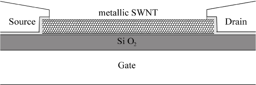
Figure 1: SWNT quantum dot setup. A metallic SWNT is coupled via tunnelling junctions to a source and a drain contact. The electrochemical potential in the dot is adjusted by a gate voltage.

So far excitation lines of SWNT quantum dots were only addressed in Oreg2000 ; Ke2003 ; Bellucci2005 in a meanfield approach. In the present work we do not only calculate the expected excitation lines but also give a quantitative calculation of the nonlinear current across a metallic SWNT quantum dot as a function of the gate and bias voltage beyond meanfield. As long as only the ground state energies are concerned, the meanfield treatment yields the right result but fails for a complete description of the excitation spectrum. Some results were already presented in abridged form in Leo2006 . We focus on the low energy regime, which means that we consider the situation where only the gapless subbands of the SWNT are relevant. Since those bands exhibit to a good approximation a linear dispersion relation, the Tomonaga-Luttinger theory can be applied. For a typical SWNT this means a range of roughly $1$ eV around the Fermi energy, which is still quite large if for example compared to the level spacing of $1.7$ meV for a noninteracting SWNT of 1 $\mu$m length.

Starting from a microscopic description of noninteracting SWNTs with open boundary conditions we include the electron - electron interactions. The resulting Hamiltonian can be diagonalized using bosonization techniques Egger1997 , obtaining the spectrum and eigenstates of the isolated metallic finite size SWNT. We apply the so called constructive bosonization procedure Haldane1981 (for a detailed review we refer to Delft1998 ), coping well with the discrete energy spectrum and especially with finite electron numbers.

The electron dynamics of the quantum dot is obtained by solving the equation of motion for the reduced density matrix (RDM) of the SWNT. The metal leads are described as equilibrated Fermi gases. Due to many-fold degenerate eigenstates of the SWNT Hamiltonian we find that offdiagonal elements (coherences) of the RDM can not be generally ignored. Apart from the degeneracy of the states, this is also a consequence of the interactions as we will show. The importance of taking into account coherences for an interacting system weakly coupled to unpolarized leads was also recently discussed in Braig 2005 , where transport through a metal grain is treated. The rates entering the master equation depend on the involved energies and on the matrix elements of the electron operators in the SWNT eigenstate basis. Noteworthy is a variation of the tunnelling amplitudes along the nanotube axis, also if only ground states are involved in transport, depending on the complete energy spectrum of the collective excitations.

The outline of this article is the following. In Section 2 we derive the master equation describing the dynamics of a generic quantum dot in second order of the tunnelling, gaining an expression for the current. In order to specify the explicit form of the master equation we derive the low energy Hamiltonian of metallic SWNTs in Section 3, and use the bosonization technique in order to diagonalize the SWNT Hamiltonian. The actual calculations for the current in the low and high bias regime are performed in Section 4.

2 Quantum dots

In this section we show how the stationary current through the system described by the Hamiltonian (1), see below, can be determined as a function of the electrochemical potentials in the leads and in the dot by calculating the dynamics of the RDM of the SWNT. Transport through the SWNT quantum dot can occur if the electrochemical potentials of source and drain are adjusted to different values by the voltages $V_{s}$ and $V_{d}.$ Since current can only flow if one transport direction is favored, the current-carrying system will have to be treated out of equilibrium beyond the linear response regime. Hence, the state of the quantum dot will in general be described by a nonequilibrium density matrix. For completeness and clarity, we show the determination of the corresponding equation of motion in some detail mainly following Blum1996 . The outcomes of this and of the following section will be used in Section 4 to obtain the $I$-$V_{b}$-$V_{g}$ characteristics of SWNT quantum dots.

2.1 Model Hamiltonian

In the following we examine the physics of a generic quantum dot, i.e. we consider a small metallic system weakly coupled to a source and a drain via tunnelling junctions. Moreover the electrochemical potential $\mu_{g}$ within the dot can be controlled by a capacitatively coupled gate voltage $V_{g}$. We describe the overall system by the Hamiltonian

$$H=H_{\odot}+H_{s}+H_{d}+H_{T}+H_{g},$$ (1)

where $H_{\odot}$ can describe an interacting SWNT (cf. equation (44) below) or another conductor with known many-body eigenstates. $H_{s/d}$ describe the isolated metallic source and drain contacts as a Fermi gas of noninteracting quasi-particles. Upon absorbing terms proportional to the external source/ drain voltage $V_{s/d}$, they read ($l=s,d$)

$$H_{l}=\sum_{\sigma\vec{q}}\varepsilon_{\vec{q},l}c_{\vec{q}\sigma l}^{\dagger}c_{\vec{q}\sigma l},$$ (2)

where $c_{\vec{q}\sigma l}^{\dagger}$ creates a quasi-particle with spin $\sigma$ and energy $\varepsilon_{\vec{q},l}=\varepsilon_{\vec{q}}-eV_{s/d}$ in lead $s/d$. The transfer of electrons between the leads and the central system is taken into account by the tunnelling Hamiltonian

$$H_{T}=\sum_{l=s,d}\sum_{\sigma}\int\textrm{d}^{3}r\left(T_{l}(\vec{r})\Psi_{\sigma}^{\dagger}(\vec{r})\Phi_{\sigma l}(\vec{r})+\textrm{h.c.}\right),$$ (3)

where $\Psi_{\sigma}^{\dagger}(\vec{r})$ and $\Phi_{\sigma l}^{\dagger}(\vec{r})=\sum_{\vec{q}}\phi_{\vec{q}}^{*}(\vec{r})c_{\vec{q}\sigma l}^{\dagger}$ are electron creation operators in the dot and in lead $l$, respectively, and $T_{l}(\vec{r})$ describes the transparency of the tunnelling contact at lead $l$. Finally, $H_{g}=-\mu_{g}\mathcal{N}_{c}=-ecV_{g}$ accounts for the gate voltage capacitively coupled to the dot, with $\mathcal{N}_{c}$ counting the total electron number in the dot and $c$ being a conversion factor, that relates the electrochemical potential to the gate voltage.

2.2 Dynamics of the reduced density matrix

Our starting point is the Liouville equation for the time evolution of the density matrix $\rho(t)$ of the system consisting of the leads and the dot. The tunnelling Hamiltonian $H_{T}$ from equation (3) is treated as perturbation. We calculate the time dependence of $\rho(t)$ in the interaction picture, i.e. we define

$$\rho^{I}(t)=U_{I}(t,t_{0})\rho(t_{0})U_{I}^{\dagger}(t,t_{0}),$$ (4)

with the time evolution operator $U_{I}(t,t_{0})$, given by

$$U_{I}(t,t_{0})=e^{\frac{i}{\hbar}\left(H_{\odot}+H_{s}+H_{d}\right)(t-t_{0})}e^{-\frac{i}{\hbar}\left(H_{\odot}+H_{s}+H_{d}+H_{T}\right)(t-t_{0})},$$ (5)

with $t_{0}$ being some reference time. Using (4) and (5) the equation of motion becomes

$$i\hbar\frac{\partial\rho^{I}(t)}{\partial t}=\left[H_{T}^{I}(t),\rho^{I}(t)\right],$$ (6)

with $H_{T}^{I}(t)=e^{\frac{i}{\hbar}\left(H_{\odot}+H_{s}+H_{d}\right)(t-t_{0})}H_{T}e^{-\frac{i}{\hbar}\left(H_{\odot}+H_{s}+H_{d}\right)(t-t_{0})}.$ Equivalently we can write

$$\rho^{I}(t)=\rho^{I}(t_{0})-\frac{i}{\hbar}\int_{t_{0}}^{t}\left[H_{T}^{I}(t_{1}),\rho(t_{1})\right]dt_{1}.$$ (7)

Reinserting (7) back into (6) yields

$$\dot{\rho^{I}}(t)=-\frac{i}{\hbar}\left[H_{T}^{I},\rho(t_{0})\right]\\ +\left(\frac{i}{\hbar}\right)^{2}\int_{t_{0}}^{t}dt_{1}\left[H_{T}^{I}(t),\left[H_{T}^{I}(t_{1}),\rho^{I}(t_{1})\right]\right].$$ (8)

Since we are interested in the transport through the central system, it is sufficient to consider the RDM $\rho_{\odot}^{I}$ of the dot, which can be obtained from $\rho^{I}$ by tracing out the lead degrees of freedom, i.e.

$$\rho_{\odot}^{I}=Tr_{\mathsf{leads}}\rho^{I}.$$ (9)

In general the leads can be considered as large systems compared to the dot. Besides we only consider the case of weak tunnelling, such that the influence of the central system on the leads is only marginal. Thus from now on we treat the leads as reservoirs which stay in thermal equilibrium and make the following ansatz to factorise the density matrix $\rho^{I}(t)$ of the total system as

$$\rho^{I}(t)=\rho_{\odot}^{I}(t)\rho_{s}\rho_{d}=:\rho_{\odot}^{I}(t)\rho_{\mathsf{leads}},$$ (10)

where $\rho_{s}$ and $\rho_{d}$ are time independent and given by the usual thermal equilibrium expression

$$\rho_{s/d}=\frac{e^{-\beta(H_{s/d}-\mu_{s/d}\mathcal{N}_{s/d})}}{Z_{s/d}},$$ (11)

with $\beta$ the inverse temperature. As it can be formally shown Blum1996 , the factorization (10) corresponds, like Fermi’s Golden Rule, to a second order treatment in the perturbation $H_{T}.$ Furthermore, we can significantly simplify equation (8) by making the so called Markov approximation (MA). The idea is that the dependence of $\dot{\rho}^{I}(t)$ on $\rho^{I}(t^{\prime})$ is only local in time. In more detail, $\rho^{I}(t^{\prime})$ is replaced by $\rho^{I}(t)$ in (8). The MA is closely connected to the correlation time $\tau$ of the leads. In our case $\tau$ is the time after which the correlation functions

$$\left\langle\Phi_{\sigma l}^{\dagger}(\vec{r},\tau)\Phi_{\sigma l}(\vec{r}^{\prime},0)\right\rangle_{\mathsf{th}}:=\\ Tr_{\mathsf{leads}}\left(\Phi_{\sigma l}^{\dagger}(\vec{r},\tau)\Phi_{\sigma l}(\vec{r}^{\prime},0)\rho_{\mathsf{leads}}\right)$$

are vanishing and therefore erasing the memory of the system. If $\rho^{I}(t^{\prime})$ is not considerably changing during $\tau$ the MA is valid. It must be noted that the MA leads to an averaging of the time evolution of $\rho^{I}(t)$ on timescales of the order of $\tau$, such that details of the dynamics on short time scales are not accessible. Since we are interested in the dc current through the system, this imposes no restriction on our purpose. Finally we get, by plugging equations (9), (10) and (11) into (8), the following expression for the equation of motion for the RDM,

$$\dot{\rho_{\odot}^{I}}(t)=-\frac{i}{\hbar}Tr_{\mathsf{leads}}\left[H_{T}^{I},\rho_{\odot}^{I}(t_{0})\rho_{\mathsf{leads}}\right]\\ +\left(\frac{i}{\hbar}\right)^{2}Tr_{\mathsf{leads}}\int_{t_{0}}^{t}dt_{1}\left[H_{T}^{I}(t),\left[H_{T}^{I}(t_{1}),\rho_{\odot}^{I}(t)\rho_{\mathsf{leads}}\right]\right].$$ (12)

The first term vanishes because $\left<\Phi_{\sigma l}(\vec{r})\right>_{\mathrm{th}}=0.$ Since we are only interested in the longterm behavior of the system we send $t_{0}\rightarrow-\infty.$ Writing out the double commutator in (12) according to

$$\left[A,\left[B,C\right]\right]=ABC+CBA-ACB-BCA,$$

and introducing the variable $t^{\prime}=t-t_{1}$ one obtains

$$\dot{\rho_{\odot}^{I}}(t)=\\ -\frac{1}{\hbar^{2}}Tr_{\mathsf{leads}}\int_{0}^{\infty}dt^{\prime}\left[\left(H_{T}^{I}(t)H_{T}^{I}(t-t^{\prime})\rho_{\odot}^{I}(t)\rho_{\mathsf{leads}}+h.c.\right)\right.\\ -\left.\left(H_{T}^{I}(t)\rho_{\odot}^{I}(t)\rho_{\mathsf{leads}}H_{T}^{I}(t-t^{\prime})+h.c.\right)\right].$$ (13)

Now we insert the explicit form of $H_{T}$ from equation (3) into (13) and perform the trace over the lead degrees of freedom. Thereby we exploit the relations

$$\left<\Phi_{\sigma l}\Phi_{\sigma l^{\prime}}\right>_{\mathrm{th}}=\left<\Phi_{\sigma l}^{\dagger}\Phi_{\sigma l^{\prime}}^{\dagger}\right>_{\mathrm{th}}=0,$$

as well as

$$\left<\Phi_{\sigma l}\Phi_{\sigma^{\prime}l^{\prime}}^{\dagger}\right>_{\mathrm{th}}=0\quad\mathrm{for}\,\sigma l\neq\sigma^{\prime}l^{\prime},$$

such that

$$\dot{\rho}_{\odot}^{I}(t)=-\frac{1}{\hbar^{2}}\sum_{l=s,d}\sum_{\sigma}\int\textrm{d}^{3}x\int\textrm{d}^{3}y\int_{0}^{\infty}dt^{\prime}\\ \left\{\left[\mathcal{E}_{\sigma l}(\vec{x},\vec{y},t^{\prime})\Psi_{\sigma}^{\dagger}(\vec{x},t)\Psi_{\sigma}(\vec{y},t-t^{\prime})\rho_{\odot}^{I}(t)\right.\right.\\ +\left.\mathcal{F}_{\sigma l}(\vec{x},\vec{y},t^{\prime})\Psi_{\sigma}(\vec{x},t)\Psi_{\sigma}^{\dagger}(\vec{y},t-t^{\prime})\rho_{\odot}^{I}(t)\right]+h.c.\\ -\left[\mathcal{F}_{\sigma l}^{*}(\vec{x},\vec{y},t^{\prime})\Psi_{\sigma}^{\dagger}(\vec{x},t)\rho_{\odot}^{I}(t)\Psi_{\sigma}(\vec{y},t-t^{\prime})\right.\\ +\left.\left.\mathcal{E}_{\sigma l}^{*}(\vec{x},\vec{y},t^{\prime})\Psi_{\sigma}(\vec{x},t)\rho_{\odot}^{I}(t)\Psi_{\sigma}^{\dagger}(\vec{y},t-t^{\prime})\right]-h.c.\right\}.$$ (14)

In (14) we have introduced

$$\mathcal{E}_{\sigma l}(\vec{x},\vec{y},t^{\prime}):=T_{l}(\vec{x})T_{l}^{*}(\vec{y})\left\langle\Phi_{\sigma l}(\vec{x})\Phi_{\sigma l}^{\dagger}(\vec{y},-t^{\prime})\right\rangle_{\mathrm{th}}=\\ T_{l}(\vec{x})T_{l}^{*}(\vec{y})\int d\varepsilon\rho_{l}^{\ominus}(\varepsilon)\sum_{\vec{q}|_{\varepsilon}}\phi_{\vec{q}}(\vec{x})\phi_{\vec{q}}^{*}(\vec{y})e^{-\frac{i}{\hbar}(\varepsilon-eV_{l})t^{\prime}},$$ (15)

with $\rho_{l}^{\ominus}(\varepsilon)=\rho_{l}(\varepsilon)(1-f(\varepsilon))$, where $\rho_{l}(\varepsilon)$ is the density of energy levels in lead $l$ and $f(\varepsilon)$ is the Fermi distribution. Similarly

$$\mathcal{F}_{\sigma l}(\vec{x},\vec{y},t^{\prime}):=T_{l}^{*}(\vec{x})T_{l}(\vec{y})\left\langle\Phi_{\sigma l}^{\dagger}(\vec{x})\Phi_{\sigma l}(\vec{y},-t^{\prime})\right\rangle_{\mathrm{th}}=\\ T_{l}^{*}(\vec{x})T_{l}(\vec{y})\int d\varepsilon\rho_{l}^{\oplus}(\varepsilon)\sum_{\vec{q}|_{\varepsilon}}\phi_{\vec{q}}^{*}(\vec{x})\phi_{\vec{q}}(\vec{y})e^{\frac{i}{\hbar}(\varepsilon-eV_{l})t^{\prime}}.$$ (16)

Here $\rho_{l}^{\oplus}(\varepsilon)=\rho_{l}(\varepsilon)f(\varepsilon).$ In order to proceed, it is convenient to represent the RDM in the eigenstate basis of the dot Hamiltonian $H_{\odot}.$ Assuming that we can diagonalize the many-body Hamiltonian $H_{\odot}$ (see Section 3), this allows us to extract the $t$ and $t^{\prime}$ dependence of the electron operators in (14). To proceed further, we carry out the following two major approximations:

I.) We assume that matrix elements between states representing different charge states vanish (the number of electrons in the dot influences the electrostatics of the whole circuit, hence is “measured” permanently).

II.) The so called secular approximation is applied, i.e. we only retain those terms of (14), which have no oscillatory behavior in $t.$ The latter causes that coherences between nondegenerate states are not present in the stationary solution of (14). For the dynamics this means that we can not resolve the evolution of $\rho_{\odot}^{I}(t)$ on time scales of $\hbar/(E_{m}-E_{n}),$ where $E_{m}$ and $E_{n}$ are two distinct energy levels of $H_{\odot}.$

In the end we can divide $\rho_{\odot}^{I}(t)$ into block matrices $\rho_{\odot}^{IE_{N}}(t),$ where $E_{N}$ denotes an energy level of the isolated dot containing $N$ electrons. To simplify the notation we give the resulting equations of motion in Bloch-Redfield form,

$$\dot{\rho}_{nm}^{I,E_{N}}(t)=-\sum_{kk^{\prime}}R_{nm\,kk^{\prime}}^{E_{N}}\rho_{kk^{\prime}}^{I,E_{N}}(t)\\ +\sum_{M=N\pm 1}\sum_{E^{\prime}}\sum_{kk^{\prime}}R_{nm\,kk^{\prime}}^{E_{N}\,E^{\prime}_{M}}\rho_{kk^{\prime}}^{I,E^{\prime}_{M}}(t),$$ (17)

where the indices $n,m,k,k^{\prime}$ refer to the eigenstates of $H_{\odot}.$ The Redfield tensors are given by $(l=s,d)$

$$R_{nm\,kk^{\prime}}^{E_{N}}=\sum_{l}\sum_{M,E^{\prime},j}\left(\delta_{mk^{\prime}}\Gamma_{l,njjk}^{(+)E_{N}\,E^{\prime}_{M}}+\delta_{nk}\Gamma_{l,k^{\prime}jjm}^{(-)E_{N}\,E^{\prime}_{M}}\right),$$ (18)

and

$$R_{nm\,kk^{\prime}}^{E_{N}\,E^{\prime}_{M}}=\sum_{l,\alpha=\pm}\Gamma_{l,k^{\prime}mnk}^{(\alpha)E^{\prime}_{M}\,E_{N}}.$$ (19)

The quantities $\Gamma_{l,k^{\prime}mnk}^{(\alpha)E_{N}\,E^{\prime}_{M}}$ determine the transitions between states with $N$ particles and energy $E_{N}$ to states with $M$ particles and energy $E^{\prime}_{M}.$ In detail we obtain for transitions $N\rightarrow N+1$

$$\Gamma_{l\,k^{\prime}mnk}^{(\alpha)E_{N}\,E^{\prime}_{N+1}}=\frac{1}{\hbar^{2}}\sum_{\sigma}\int d^{3}x\int d^{3}y\times\\ \left(\Psi_{\sigma}(\vec{x})\right)_{k^{\prime}m}^{E_{N}\,E^{\prime}_{N+1}}\left(\Psi_{\sigma}^{\dagger}(\vec{y})\right)_{nk}^{E^{\prime}_{N+1}\,E_{N}}\times\\ \int_{0}^{\infty}dt^{\prime}\mathcal{F}_{\sigma l}(\vec{x},\vec{y},t^{\prime})e^{-\alpha\frac{i}{\hbar}\left(E^{\prime}_{N+1}-E_{N}\right)t^{\prime}}.$$ (20)

For transitions $N\rightarrow N-1$ is

$$\Gamma_{l\,k^{\prime}mnk}^{(\alpha)E_{N}\,E_{N-1}}=\frac{1}{\hbar^{2}}\sum_{\sigma}\int d^{3}x\int d^{3}y\times\\ \left(\Psi_{\sigma}^{\dagger}(\vec{x})\right)_{k^{\prime}m}^{E_{N}\,E^{\prime}_{N-1}}\left(\Psi_{\sigma}(\vec{y})\right)_{nk}^{E^{\prime}_{N-1}\,E_{N}}\times\\ \int_{0}^{\infty}dt^{\prime}\mathcal{E}_{\sigma l}(\vec{x},\vec{y},t^{\prime})e^{-\alpha\frac{i}{\hbar}\left(E^{\prime}_{N-1}-E_{N}\right)t^{\prime}},$$ (21)

where we have defined the matrix elements

$$\left(\Psi_{\sigma}^{\dagger}(\vec{x})\right)_{km}^{E_{N}\,E^{\prime}_{N+1}}:=\left\langle k\left|\Psi_{\sigma}^{\dagger}(\vec{x})\right|m\right\rangle,$$ (22)

with the states $\left|k\right\rangle$ and $\left|m\right\rangle$ having energy $E_{N},\,E^{\prime}_{N+1}$ and particle number $N,\,N+1$ respectively.

Equation (17) governs the dynamics of the SWNT electrons. In the following we deduce therefrom the current through the system.

2.3 Current

The current is essentially the net tunnelling rate in a certain direction at one of the leads. Thus the current at lead $l$ will be of the form

$$I_{l}=le\sum_{N}\left(\Sigma_{l}^{N\rightarrow N+1}-\Sigma_{l}^{N\rightarrow N-1}\right),$$ (23)

where we use the convention $l=s/d=\pm 1.$ On the long run the currents at the two leads have to be equal, otherwise charge would accumulate on the dot which is prevented by the charging energy. The rates $\Sigma_{l}^{N\rightarrow N\pm 1}$ can be obtained from the time evolution of the occupation probabilities $P_{N}=Tr\left(\rho_{\odot}^{I,N}\right)$, where $\rho_{\odot}^{I,N}$ is the RDM for states containing $N$ electrons. In more detail, the occupation probability of the charge state $N$ is reduced by tunnelling events changing the number of electrons from $N$ to $N\pm 1$ and is increased by processes transferring the charge states $N\pm 1$ to $N,$ hence

$$\dot{P}_{N}=Tr\left(\dot{\rho}_{\odot}^{I,N}\right)=\\ \sum_{l}\left(-\Sigma_{l}^{N\rightarrow N+1}-\Sigma_{l}^{N\rightarrow N-1}+\Sigma_{l}^{N+1\rightarrow N}+\Sigma_{l}^{N-1\rightarrow N}\right).$$

Using $Tr\left(\dot{\rho}_{\odot}^{I,N}\right)=\sum_{E}Tr\left(\dot{\rho}_{\odot}^{I,E_{N}}\right)$ together with (17) we can easily identify the rates appearing in (23):

$$\Sigma_{l}^{N\rightarrow N\pm 1}=\\ \sum_{E,E^{\prime}}\sum_{nkj}\left(\Gamma_{l,njjk}^{(+)E_{N}\,E^{\prime}_{N\pm 1}}\rho_{kn}^{I,E_{N}}+\rho_{nk}^{I,E_{N}}\Gamma_{l,kjjn}^{(-)E_{N}\,E^{\prime}_{N\pm 1}}\right).$$ (24)

Since the relation $\Gamma_{l,njjk}^{(+)E_{N}\,E^{\prime}_{N\pm 1}}=\left(\Gamma_{l,kjjn}^{(-)E_{N}\,E^{\prime}_{N\pm 1}}\right)^{*}$ holds, we arrive, by inserting (24) into (23), at the following expression,

$$I_{l}=\\ l2e\mathrm{Re}\sum_{N,E,E^{\prime}}\left(\Gamma_{l,njjk}^{(+)E_{N}\,E^{\prime}_{N+1}}-\Gamma_{l,njjk}^{(+)E_{N}\,E^{\prime}_{N-1}}\right)\rho_{kn\ }^{I,E_{N}}.$$ (25)

For the actual calculations we are going to replace $\rho^{I,E_{N}}$ in (25) by the stationary solution $\rho_{st}^{I,E_{N}}$ of (14), because we are only interested in the longterm behavior of the system.

Until now our treatment has been quite general, having made no assumptions about the nature of the dot so far. But the actual transport properties depend on the microscopic structure of the system. As seen from equations (20) and (21), we shall have to determine the spectrum of $H_{\odot}$ and the matrix elements $\left(\Psi_{\sigma}(\vec{x})\right)_{kk^{\prime}}^{E_{N}\,E^{\prime}_{N\pm 1}}$ in order to solve master equation (17). This is the subject of the next section. Moreover the leads and the geometry of the tunnelling contacts will influence the system via the quantities $\mathcal{F}_{\sigma l}$ and $\mathcal{E}_{\sigma l}$ as discussed in Section 4.1 and Appendix A.

3 Low energy description of metallic finite size SWNTs

In the following we derive the Hamiltonian $H_{\odot}$ describing the interacting electrons in a metallic finite size SWNT at low energies. Typically (depending on the diameter of the nanotube) “low energies” mean a range of 1 eV around the Fermi energy, such that the dispersion relation for the noninteracting electrons is linear Egger1997 around the Fermi points. Since we are interested in the transport across a finite size system, open boundary conditions (OBCs) for the wave functions must be imposed and we can deduce the wave functions and the energy spectrum of the noninteracting system. Switching on interactions we still can diagonalize the Hamiltonian by using the so called constructive bosonization procedure Haldane1981 ; Delft1998 , which we also employ in order to rewrite the electron operators in a suitable form for the determination of the matrix elements $\left(\Psi_{\sigma}(\vec{x})\right)_{kk^{\prime}}^{E_{N}\,E^{\prime}_{N+1}}$.

3.1 Noninteracting SWNTs

The bandstructure of SWNTs is conveniently derived from the one of the unbound $2p_{z}$ electrons in graphene sheets Saito1998 . Since each unit cell of the graphene lattice contains two atoms $p=1,2$, the band structure consists of a valence and a conduction band which touch at the corner points of the first Brillouin zone. Two of those Fermi points, $F=\pm\vec{K}_{0}$, are independent, i.e. don’t differ by a reciprocal lattice vector. The energy dispersion around the Fermi points is very well linearly approximated with a Fermi velocity $v_{F}=8.1\cdot 10^{5}\,m/s$. Since SWNTs are essentially graphene sheets rolled up to a cylinder of a certain diameter, we obtain the SWNT band structure by imposing periodic boundary conditions around the circumference $L_{\perp}$ of the tube, leading to the quantization of the allowed transverse wave vectors

$$k_{\perp}=\frac{2\pi}{L_{\perp}}m,\quad m=0,\pm 1,\pm 2\dots\quad,$$ (26)

and thus to the formation of subbands labelled by $m.$ For metallic SWNTs the Fermi points $F$ will satisfy condition (26), hence the corresponding valence and conduction subbands will have no gap. In the following the focus is on armchair SWNTs. Then only the gapless sub-bands with linear energy dispersion nearby the Fermi points are relevant Egger1997 ; Kane1997 . At each Fermi point there are two different branches $r=R/L$ associated to right and left moving electrons. The corresponding Bloch waves are of the form

$$\varphi_{R/L,F,\kappa}(\vec{r})=e^{i\kappa x}\varphi_{R/L,F}(\vec{r}),$$ (27)

where $\kappa$ measures the distance from the Fermi points $\pm\vec{K}_{0}$ (Fig. 2 left).

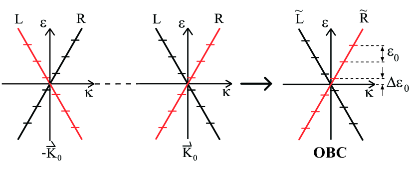
Figure 2: On the right, energy spectrum of a SWNT with open boundary conditions (OBCs) described in terms of left ($\tilde{L}$) and right ($\tilde{R}$) branches. It is constructed from suitable combinations of travelling waves (cf. equation (29)) whose spectrum is shown on the left side.

In more detail, the Bloch waves $\varphi_{R/L,F}(\vec{r})$ at the Fermi points are given by a superposition of wave functions living either on sublattice $p=1$ or $p=2,$

$$\varphi_{R/L,F}(\vec{r})=\frac{1}{\sqrt{N_{L}}}\sum_{\vec{R},p}e^{iF\cdot\vec{R}}f_{prF}\chi(\vec{r}-\vec{R}-\vec{\tau}_{p}),$$ (28)

where $N_{L}$ is the number of lattice sites which are identified by the lattice vector $\vec{R}.$ The position of the atoms $p=1,\ 2$ in the unit cell is given by $\tau_{p}$ and the functions $\chi$ are the $p_{z}$ orbitals. The value of the coefficients $f_{prF}$ depends on the considered SWNT type. For simplicity we concentrate on armchair SWNTs for which we have $f_{1rF}=1/\sqrt{2},\,f_{2rF}=-1/\sqrt{2}\mathrm{sgn}(rF),$ where we use the convention that $R/L=\pm 1.$ In this article, we are interested in finite size effects and therefore we impose OBCs instead of periodic boundary conditions on the single electron wave functions. Generalizing Fabrizio1995 to the case of SWNTs we introduce standing waves which fulfil the OBCs (Fig. 2 right):

$$\varphi_{\tilde{R}/\tilde{L},\kappa}^{OBC}(\vec{r})=\frac{1}{\sqrt{2}}\left[\varphi_{R/L,K_{0},\kappa}(\vec{r})-\varphi_{L/R,-K_{0},-\kappa}(\vec{r})\right]\;,$$ (29)

with quantization condition

$$\kappa=\pi(m_{\kappa}+\Delta)/L,\quad m_{\kappa}=0,\pm 1,\pm 2,\dots,$$

where $L$ is the SWNT length. The offset parameter $\Delta$ occurs if there is no integer $n$ with $\vec{K}_{0}=(\pi n/L)\hat{e}_{\parallel}$ (where $\hat{e}_{\parallel}$ is the unit vector along the tube axis) and is responsible for a possible energy mismatch between the states of the $\tilde{R}$ and $\tilde{L}$ branches, defined by relation (29). From the linear energy dispersion relation around the Fermi points, the energies of the standing waves follow as

$$\varepsilon_{\tilde{r}\kappa}=\mathrm{sgn}(\tilde{r})\hbar v_{F}\kappa.$$ (30)

Including the spin degree of freedom, the electron operator reads

$$\Psi(\vec{r})=\sum_{\tilde{r}=\tilde{R},\tilde{L}}\sum_{\kappa,\sigma}\varphi_{\tilde{r}\kappa}^{OBC}(\vec{r})c_{\tilde{r}\sigma\kappa}=:\sum_{\sigma}\Psi_{\sigma}(\vec{r}),$$ (31)

where the operator $c_{\tilde{r}\sigma\kappa}$ annihilates the state $\left|\varphi_{\tilde{r}\kappa}^{OBC}\right\rangle\left|\sigma\right\rangle$. Since the Bloch waves can be divided into a slowly and a fast oscillating part (cf. (27)) we can as well split off a slowly varying part from the operators $\Psi_{\sigma}(\vec{r}),$ i.e. we introduce the 1D operators

$$\psi_{\tilde{r}\sigma F}(x)=\frac{1}{\sqrt{2L}}\sum_{\kappa}e^{i\mathrm{sgn}(F)\kappa x}c_{\tilde{r}\sigma\kappa},$$ (32)

in terms of which the 3D electron operators read

$$\Psi_{\sigma}(\vec{r})=\sqrt{L}\sum_{F}\mathrm{sgn}(F)\times\\ \left[\varphi_{\mathrm{sgn}(F)R,F}(\vec{r})\psi_{\tilde{R}\sigma F}(x)+\varphi_{\mathrm{sgn}(F)L,F}(\vec{r})\psi_{\tilde{L}\sigma F}(x)\right].$$ (33)

Later on, the bosonizability of $\psi_{\tilde{r}\sigma F}(x)$ will be of quite some significance for the calculation of the transport properties.

From (30) the appropriate Hamiltonian for the noninteracting system is easily derived. It reads

$$H_{\odot,0}=\hbar v_{F}\sum_{\tilde{r}\sigma}\mathrm{sgn}(r)\sum_{\kappa}\kappa c_{\tilde{r}\sigma\kappa}^{\dagger}c_{\tilde{r}\sigma\kappa}.$$ (34)

3.2 Interacting SWNTs

For the inclusion of the electron - electron interactions we have to add the following term to the SWNT Hamiltonian,

$$V_{\odot}=\\ \frac{1}{2}\sum_{\sigma\sigma^{\prime}}\int d^{3}r\int d^{3}r^{\prime}\Psi_{\sigma}^{\dagger}(\vec{r})\Psi_{\sigma^{\prime}}^{\dagger}(\vec{r}^{\prime})V(\vec{r}-\vec{r}^{\prime})\Psi_{\sigma^{\prime}}(\vec{r}^{\prime})\Psi_{\sigma}(\vec{r}),$$ (35)

where $V(\vec{r}-\vec{r}^{\prime})$ is the possibly screened Coulomb potential. Upon inserting (33) into (35), integration over the coordinates perpendicular to the tube axis yields the interacting Hamiltonian expressed in terms of 1D operators and an effective 1D interaction $V_{\mathrm{eff}}(x,x^{\prime}),$ see (37) below. As in Egger1997 we expand the Bloch waves into their sublattice contributions (28) and ignore the difference between the intra and inter lattice correlations, which are only of relevance at the length scale of the next neighbor spacing of the carbon atoms. The final form of $V_{\odot}$ we obtain by ignoring all fast oscillating terms in the interaction, or in other words by keeping only the so called forward scattering processes associated to the effective potential $V_{\mathrm{eff}}$ as depicted in Fig. 3. This leads to an expression of $V_{\odot}$ in terms of the 1D densities $\rho_{\tilde{r}\sigma F}(x)=\psi_{\tilde{r}\sigma F}^{\dagger}(x)\psi_{\tilde{r}\sigma F}(x),$

$$V_{\odot}=\\ \frac{1}{2}\sum_{\tilde{r}\tilde{r}^{\prime}}\sum_{FF^{\prime}}\sum_{\sigma\sigma^{\prime}}\int\int_{0}^{L}dxdx^{\prime}\rho_{\tilde{r}\sigma F}(x)V_{\mathrm{eff}}(x,x^{\prime})\rho_{\tilde{r}^{\prime}\sigma^{\prime}F^{\prime}}(x^{\prime}).$$ (36)

The approximations that have been made for getting from (35) to (36) mainly mean that we neglect, as already mentioned in the introduction, any kind of exchange effects and thus are only valid for large enough SWNTs. Using (28) and (31) the effective potential $V_{\mathrm{eff}}$ is obtained from an integral over the coordinates perpendicular to the tube axis of the 3D Coulomb interaction weighted by the $p_{z}$ orbitals, i.e.

$$V_{\mathrm{eff}}(x,x^{\prime})=\frac{L^{2}}{N_{L}^{2}}\times\\ \sum_{\vec{R},\vec{R}^{\prime}}\int d^{2}r_{\perp}\int d^{2}r^{\prime}_{\perp}\left|\chi(\vec{r}-\vec{R})\right|^{2}V(\vec{r}-\vec{r}^{\prime})\left|\chi(\vec{r}^{\prime}-\vec{R}^{\prime})\right|^{2}.$$ (37)

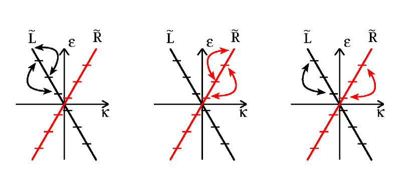
Figure 3: Scheme of forward scattering terms. All those processes conserve the number of electrons in each branch.

3.3 Bosonization

Here we show how the introduction of bosonic excitations enables us to diagonalize the SWNT Hamiltonian $H_{\odot}=H_{\odot,0}+V_{\odot}$ by recasting it into a sum of a fermionic and a bosonic part. Besides we give the identity that expresses the electron operators in terms of the boson operators. The connection between fermionic and bosonic operators can be obtained from the Fourier coefficients of the electron density operators. To be more specific, we Fourier expand the electron density operator,

$$\rho_{\tilde{r}\sigma F}(x)=\frac{1}{2L}\sum_{q}e^{i\mathrm{sgn}(F)qx}\rho_{\tilde{r}\sigma q},$$ (38)

with $q=\frac{\pi}{L}n_{q},\,n_{q}\in\mathbb{Z}$ and define the operators

$$b_{\sigma\mathrm{sgn}(\tilde{r})q}=\frac{1}{\sqrt{n_{q}}}\rho_{\tilde{r}\sigma\mathrm{sgn}(\tilde{r})q},\quad q>0.$$ (39)

The operators $b_{\sigma q}$ fulfil the canonical bosonic commutation relations $\left[b_{\sigma q},b_{\sigma^{\prime}q^{\prime}}^{\dagger}\right]=\delta_{\sigma\sigma^{\prime}}\delta_{qq^{\prime}}$ as it can be shown Delft1998 by using the explicit expression

$$b_{\sigma\mathrm{sgn}(\tilde{r})q}=\frac{1}{\sqrt{n_{q}}}\sum_{\kappa}c_{\tilde{r}\sigma\kappa}^{\dagger}c_{\tilde{r}\sigma\kappa+\mathrm{sgn}(\tilde{r})q},\quad q>0.$$ (40)

From the previous equation we can see that the $b,\,b^{\dagger}$ operators annihilate or create collective particle hole excitations within the branch $(\tilde{r}\sigma)$.

3.3.1 Diagonalization of the SWNT Hamiltonian

As for example shown in Delft1998 for a generic 1D system, the noninteracting part of the Hamiltonian is already diagonal in the bosonic operators. For the SWNTs in particular, we obtain from (34) and (40),

$$H_{\odot,0}=\\ \varepsilon_{0}\sum_{\sigma}\left[\sum_{q\neq 0}\left|n_{q}\right|b_{\sigma q}^{\dagger}b_{\sigma q}+\sum_{\tilde{r}}\left(\frac{1}{2}\mathcal{N}_{\tilde{r}\sigma}^{2}+\Delta\mathrm{sgn}(\tilde{r})\mathcal{N}_{\tilde{r}\sigma}\right)\right],$$ (41)

where $\varepsilon_{0}=\hbar v_{F}\frac{\pi}{L}$ is the level spacing of the noninteracting nanotube. The first term in (41) describes collective particle hole excitations, whereas the second term represents the energy cost of the shell filling due to Pauli’s principle. Specifically, $\mathcal{N}_{\tilde{r}\sigma}=\sum_{\kappa}c_{\tilde{r}\sigma\kappa}^{\dagger}c_{\tilde{r}\sigma\kappa}$ counts the number of electrons $N_{\tilde{r}\sigma}$ in the $(\tilde{r}\sigma)$-branch. Without loss of generality we have assumed that we only have states with a positive number of particles in each branch.

Plugging the Fourier expansion of the density operators (38) into (36) and taking into account the definition of the $b$-operators yields the bosonized form of $V_{\odot},$

$$V_{\odot}=\frac{1}{2}E_{c}\mathcal{N}_{c}^{2}+\frac{1}{2}\sum_{q>0}n_{q}W_{qq}\times\\ \sum_{\sigma\sigma^{\prime}}\sum_{\tilde{r}\tilde{r}^{\prime}}\left(b_{\sigma\mathrm{sgn}(\tilde{r})q}+b_{\sigma\mathrm{sgn}(\tilde{r})q}^{\dagger}\right)\left(b_{\sigma^{\prime}\mathrm{sgn}(\tilde{r}^{\prime})q}+b_{\sigma^{\prime}\mathrm{sgn}(\tilde{r}^{\prime})q}^{\dagger}\right).$$ (42)

Here $E_{c}=W_{00}$ is the SWNT charging energy responsible for the Coulomb blockade and the effective interaction potential is absorbed into

$$W_{qq}=\frac{1}{L^{2}}\int_{0}^{L}dx\int_{0}^{L}dx^{\prime}V_{\mathrm{eff}}(x,x^{\prime})\cos(qx)\cos(qx^{\prime}).$$ (43)

Since the bosonic operators appear only quadratically in (41) and (42), the Bogoliubov transformation Avery1976 can be applied to diagonalize the bosonic part of the total SWNT Hamiltonian. Here we only give the result, namely

$$H_{\odot} = \frac{1}{2}E_{c}\mathcal{N}_{c}^{2}+\varepsilon_{0}\sum_{\tilde{r}\sigma}\left(\frac{\mathcal{N}_{\tilde{r}\sigma}^{2}}{2}+\Delta\textrm{sgn}(\tilde{r})\mathcal{N}_{\tilde{r}\sigma}\right)$$ (44)

$$+ \sum_{q>0}\sum_{j=c,s}\sum_{\delta=\pm}\varepsilon_{j\delta q}a_{j\delta q}^{\dagger}a_{j\delta q}.$$

The first line of (44) describes the energy cost to add new particles to the system. The excitations are created by the bosonic operators $a_{j\delta q}^{\dagger}$. Four channels are associated to total ($j\delta=c+$, $s+$) and relative $(j\delta=c-,s-)$ (with respect to the occupation of the $\tilde{R}$ and $\tilde{L}$ branch) charge and spin excitations. To be more precise, the new operators $a_{j\delta q}$ are related to the old operators $b_{\sigma\mathrm{sgn}(\tilde{r})q}$ via the Bogoliubov transformation:

$$b_{\sigma\mathrm{sgn}(\tilde{r})q}=\sum_{j\delta}\Lambda_{\tilde{r}\sigma}^{j\delta}\left(S_{j\delta q}a_{j\delta q}+C_{j\delta q}a_{j\delta q}^{\dagger}\right),$$ (45)

where $\Lambda_{\sigma\tilde{r}}^{j\delta}$ is given by

$$\Lambda_{\tilde{r}\sigma}^{j\delta}=\frac{1}{2}\left(\begin{array}[]{cccc}1&1&1&1\\ 1&1&-1&-1\\ 1&-1&1&-1\\ 1&-1&-1&1\end{array}\right),\quad\begin{array}[]{cc}j\delta=&c+,c-,s+,s\\ \tilde{r}\sigma=&\tilde{R}\uparrow,\tilde{R}\downarrow,\tilde{L}\uparrow,\tilde{L}\downarrow\end{array}.$$ (46)

For the transformation indices $S_{j\delta q}$ and $C_{j\delta q}$ we get in the case of the three modes $j\delta=c-,s+,s-$,

$$S_{j\delta q}=1\textrm{ and }C_{j\delta q}=0.$$ (47)

Only for $j\delta=c+$ there is an interaction dependence,

$$S_{c+q}=\frac{1}{2}\left(\sqrt{\frac{\varepsilon_{0q}}{\varepsilon_{cq}}}+\sqrt{\frac{\varepsilon_{cq}}{\varepsilon_{0q}}}\right),\,C_{c+q}=\frac{1}{2}\left(\sqrt{\frac{\varepsilon_{0q}}{\varepsilon_{cq}}}-\sqrt{\frac{\varepsilon_{cq}}{\varepsilon_{0q}}}\right).$$ (48)

Generalized spin-charge separation occurs, since for the three interaction independent channels $j\delta=c-,s+,s-$ the energy dispersion is the same as for the noninteracting system,

$$\varepsilon_{j\delta q}=\hbar v_{F}q=\hbar v_{F}\frac{\pi}{L}n_{q}=:\varepsilon_{0q},\quad n_{q}=1,2,\dots\quad,$$

but the energies of the $c+$ channel are enhanced by the repulsive interaction,

$$\varepsilon_{c+\,q}=\varepsilon_{0q}(1+8W_{qq}/\varepsilon_{0})^{1/2}.$$ (49)

The ratio between $\varepsilon_{c+\,q}$ and $\varepsilon_{0\,q}$ for a (20,20)-armchair SWNT is shown in Fig. (4). For the actual calculation of $\varepsilon_{c+\,q}$ we have substituted $\left|\chi(\vec{r}-\vec{R})\right|^{2}$ by $\delta(\vec{r}-\vec{R})$ in (37). The extension of the $p_{z}$ orbitals has been modeled by introducing the average distance $a_{\perp}\approx 0.15$ nm of the electrons from their nuclei Egger1997 , i.e. we used for the 3D interaction potential the following expression

$$V(\vec{R}-\vec{R}^{\prime})=\frac{e^{2}}{4\pi\varepsilon_{0}\varepsilon}\frac{e^{-\left|\vec{R}-\vec{R}^{\prime}\right|/L_{\textrm{screen}}}}{\sqrt{\left(\vec{R}-\vec{R}^{\prime}\right)^{2}+a_{\perp}^{2}}}.$$

Here $L_{\textrm{screen}}$ is the screening length of the potential and $\varepsilon_{0}\varepsilon$ is the dielectric constant. Due to the finite range of the interaction potential we find a decay of $\varepsilon_{c+\,q}/\varepsilon_{0\,q}$ with increasing $q,$ which should be taken into account if higher excitations in the $c+$ channel are involved in transport. In the Luttinger liquid theory $\varepsilon_{c+\,q}/\varepsilon_{0\,q}$ is usually assumed to be equal to the constant $1/g,$ where

$$g=(1+8W_{qq}/\varepsilon_{0})^{-1/2},\quad q=\frac{\pi}{L}.$$ (50)

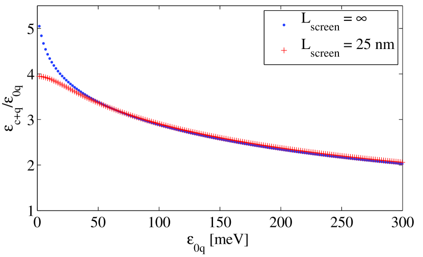
Figure 4: The ratio $\varepsilon_{c+\,q}/\varepsilon_{0\,q}$ as a function of $\varepsilon_{0\,q}$ for a (20,20) armchair SWNT of 980 nm length. Here we show the decay of $\varepsilon_{c+\,q}/\varepsilon_{0\,q}$ for an unscreened and a screened (screening length 25 nm) Coulomb interaction. In both cases, a dielectric constant $\varepsilon$ of $1.4$, see Ref. Egger1997 , is assumed.

The eigenstates of the SWNT Hamiltonian in (44) are

$$\left|\vec{N},\vec{m}\right\rangle:=\prod_{q>0,j\delta}\left(m_{j\delta q}!\right)^{-1/2}\left(a_{j\delta q}^{\dagger}\right)^{m_{j\delta q}}\left|\vec{N},\vec{0}\right\rangle,$$ (51)

where $|\vec{N},\vec{0}\rangle$ has no bosonic excitations and the vector $\vec{N}$ defines the number of electrons in each of the four branches $(\tilde{r}\sigma).$

3.3.2 Bosonization of the electron operators

The determination of the transport properties through the SWNT quantum dot involves the calculation of the matrix elements of the electron operators between the eigenstates (51). Therefor we give the so called bosonization identity for the operators $\psi_{\tilde{r}\sigma F}(x)$,

$$\psi_{\tilde{r}\sigma F}(x)=\frac{1}{\sqrt{1-e^{-\alpha\frac{\pi}{L}}}}\eta_{\tilde{r}\sigma}K_{\tilde{r}\sigma F}(x)e^{i\phi_{\tilde{r}\sigma F}^{\dagger}(x)+i\phi_{\tilde{r}\sigma F}(x)}.$$ (52)

The way (52) is derived can be found e.g. in Delft1998 . Here $\alpha$ is a convergence factor needed to ensure that only excitations with physically sensible energies are considered. It will be set to zero at the end of the calculation. The operator $\eta_{\tilde{r}\sigma}$ is the so called Klein factor. Its main effect if acting on a state $\left|\vec{N},\vec{m}\right\rangle$ is to annihilate a particle in the $(\tilde{r}\sigma)$-branch, more precisely

$$\eta_{\tilde{r}\sigma}\left|\vec{N},\vec{m}\right\rangle=(-1)^{\sum_{j=1}^{\tilde{r}\sigma-1}N_{j}}\left|\vec{N}-\hat{e}_{\tilde{r}\sigma},\vec{m}\right\rangle,$$

where we use the convention $j=\tilde{R}\uparrow,\tilde{R}\downarrow,\tilde{L}\uparrow,\tilde{L}\downarrow$ $=1,2,3,4$. The fact that the Klein factor annihilates fermions after all, expresses itself in the factor $(-1)^{\sum_{j=1}^{\tilde{r}\sigma-1}N_{j}}.$ $K_{\tilde{r}\sigma F}(x)$ yields a phase depending on the number of electrons in the $(\tilde{r}\sigma)$ branch, in our case,

$$K_{\tilde{r}\sigma F}(x)=\frac{1}{\sqrt{2L}}e^{i\frac{\pi}{L}\mathrm{sgn}(F)(\mathrm{sgn}(\tilde{r})\mathcal{N}_{\tilde{r}\sigma}+\Delta)x}.$$

At last we have the fields $\phi_{r\sigma F}(x)$ given in terms of the bosonic operators $b_{\sigma q},$

$$i\phi_{r\sigma F}(x)=\sum_{q>0}\frac{e^{-\alpha q/2}}{\sqrt{n_{q}}}e^{i\mathrm{sgn}(\tilde{r}F)qx}b_{\sigma\mathrm{sgn}(\tilde{r})q}.$$

3.3.3 The matrix elements of the electron operators

In the following we are going to determine the matrix elements $\left(\Psi_{\sigma}(\vec{x})\right)_{kk^{\prime}}^{E_{N}\,E^{\prime}_{N\pm 1}}$, appearing in the transition rates (20) and (21). As we know from equation (33) the 3D electron operators $\Psi_{\sigma}(\vec{x})$ can be written in terms of the 1D operators $\psi_{r\sigma F}(x)$ yielding

$$\left(\Psi_{\sigma}(\vec{x})\right)_{kk^{\prime}}^{E_{N}\,E^{\prime}_{N\pm 1}}=\sqrt{L}\sum_{F}\mathrm{sgn}(F)\times\\ \left[\varphi_{\mathrm{sgn}(F)R,F}(\vec{r})\left(\psi_{\tilde{R}\sigma F}(x)\right)_{kk^{\prime}}^{E_{N}\,E^{\prime}_{N\pm 1}}\right.\\ +\left.\varphi_{\mathrm{sgn}(F)L,F}(\vec{r})\left(\psi_{\tilde{L}\sigma F}(x)\right)_{kk^{\prime}}^{E_{N}\,E^{\prime}_{N\pm 1}}\right].$$ (53)

Now the bosonization procedure used for the diagonalization of $H_{\odot}$ and the redefinition of $\psi_{r\sigma F}(x)$ in terms of boson operators pays off. Denoting the SWNT eigenstates $\left|k\right\rangle$ and $\left|k^{\prime}\right\rangle$ as $\left|\vec{N},\vec{m}\right\rangle$ and $\left|\vec{N}^{\prime},\vec{m}^{\prime}\right\rangle$ according to equation (51), we get, as shown in Appendix B,

$$\left\langle\vec{N},\vec{m}\right|\psi_{\tilde{r}\sigma F}(x)\left|\vec{N}^{\prime},\vec{m}^{\prime}\right\rangle=\delta_{\vec{N}+\hat{e}_{\tilde{r}\sigma},\vec{N}^{\prime}}(-1)^{\sum_{j=1}^{\tilde{r}\sigma-1}N_{j}}\times\\ K_{\tilde{r}F(\vec{N}^{\prime})_{\tilde{r}\sigma}}(x)\underbrace{\frac{e^{-\frac{1}{2}\sum_{q>0}e^{-\alpha q}\sum_{j\delta}\left|\lambda_{\tilde{r}\sigma F}^{j\delta q}(x)\right|^{2}}}{\sqrt{1-e^{-\alpha\frac{\pi}{L}}}}}_{=:A(x)}\times\\ \prod_{q>0}\prod_{j\delta}F(\lambda_{\tilde{r}\sigma F}^{j\delta q}(x),m_{j\delta q},m^{\prime}_{j\delta q}).$$ (54)

The parameters $\lambda_{\tilde{r}\sigma F}^{j\delta q}(x)$ (cf. Appendix C) for the three neutral modes $j\delta=c-,\ s+,\ s-$ are given by

$$\lambda_{\tilde{r}\sigma F}^{j\delta q}(x)=\frac{e^{i\mathrm{sgn}(F\tilde{r})qx}}{\sqrt{n_{q}}}\Lambda_{\tilde{r}\sigma}^{j\delta},$$ (55)

and for the $c+$ mode we have

$$\lambda_{\tilde{r}\sigma F}^{c+q}(x)=\\ \frac{1}{2\sqrt{n_{q}}}\left(\sqrt{\frac{\varepsilon_{cq}}{\varepsilon_{0q}}}\cos(qx)+i\sqrt{\frac{\varepsilon_{0q}}{\varepsilon_{cq}}}\mathrm{sgn}(F\tilde{r})\sin(qx)\right).$$ (56)

The function $F(\lambda,m,m^{\prime})$, describing the dependence of the matrix elements on the bosonic excitations, can be expressed in terms of the Laguerre polynomials $L_{n}^{m}$ as we show explicitly in Appendix B, see equations (93) and (94) there. It is interesting to note that the interaction leads to the formation of a non-oscillatory $x$ dependence of the matrix elements $\left\langle k\left|\psi_{\tilde{r}\sigma F}(x)\right|k^{\prime}\right\rangle.$ For matrix elements between states with no bosonic $c+$ excitations this effect is described solely by the function $A(x)$. From expressions (55) and (56) for the parameters $\lambda_{\tilde{r}\sigma F}^{j\delta q}$ we find

$$A(x)=e^{-\sum_{q>0}\frac{e^{-\alpha q}}{8n_{q}}\left(\frac{\varepsilon_{cq}}{\varepsilon_{0q}}\cos^{2}(qx)+\frac{\varepsilon_{0q}}{\varepsilon_{cq}}\sin^{2}(qx)-1\right)}.$$ (57)

Since we are considering a finite ranged interaction, the ratio $\varepsilon_{cq}/\varepsilon_{0q}$ goes to $1$ for large $q$ and so the sum in (57) converges even for $\alpha=0$ (using a finite $\alpha$ in order to disregard unphysical states outside of the low energy regime has only little effect on $A(x)$). In Fig. 5 we show $A(x)$ for a (20,20) armchair SWNT with screened and unscreened Coulomb potential, using the values of $\varepsilon_{cq}/\varepsilon_{0q}$ as shown in Fig. (4). It is evident that $A(x)$ (and hence the tunnelling amplitude at low energies) is smallest at the tube ends and increases towards the middle of the nanotube. For an attractive interaction the opposite behavior would be found and for the noninteracting system $A(x)\equiv 1.$ Hence $A(x)$ is closely related to the dispersion relation for the excitation energies $\varepsilon_{cq}$. However, in this article the contact geometry is fixed and so the actual form of $A(x)$ doesn’t influence the transport properties qualitatively, as we will show below when discussing the role of the tunnelling contacts.

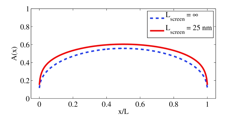
Figure 5: The non-oscillatory position dependence of the matrix elements $\left\langle k\left|\psi_{\tilde{r}\sigma F}(x)\right|k^{\prime}\right\rangle$ is described by $A(x),$ if no $c+$ excitations are involved. For a repelling interaction, $A(x)$ is strongly suppressed at the SWNT ends. Here we used the values of $\varepsilon_{cq}/\varepsilon_{0q}$ of a (20,20) armchair SWNT ($L=980$ nm) as shown in Fig. (4).

4 Current through a SWNT quantum dot

Knowing the spectrum of $H_{\odot}$ and the expressions for the electron operator matrix elements we can return to Section 2.2 and perform the actual calculation of the current through a SWNT quantum dot.

4.1 Influence of the tunnelling contacts

Due to the integration $\int d^{3}x\int d^{3}y$, the rates from (20) and (21) depend on the geometry of the tunnelling contact. At low enough energies (i.e. as long as no degenerate states with very different bosonic excitations or fermionic configurations are considered), the matrix elements of the 1D operators are slowly varying compared to the extension of the tunnelling contacts described by the transparencies $T_{l}(\vec{r}).$ Then the influence of the tunnelling contacts at the tube ends can be taken into account by introducing the parameters (cf. Appendix A)

$$\Phi_{l\tilde{r}\tilde{r}^{\prime}}(\varepsilon)=\\ \int d^{3}r\int d^{3}r^{\prime}T_{l}^{*}(\vec{r})T_{l}(\vec{r^{\prime}})\sum_{\vec{q}|_{\varepsilon}}\phi_{l\vec{q}}^{*}(\vec{r})\phi_{l\vec{q}}(\vec{r^{\prime}})A(x)A(x^{\prime})\\ \times\sum_{FF^{\prime}}\mathrm{sgn}(FF^{\prime})\varphi_{\mathrm{sgn}(F)r,F}(\vec{r})\varphi_{\mathrm{sgn}(F^{\prime})r^{\prime},F^{\prime}}^{*}(\vec{r}^{\prime})\nu_{lFF^{\prime}}(\Delta),$$ (58)

where the phase factor $\nu_{lFF^{\prime}}(\Delta)=e^{i\delta_{l,d}\pi\mathrm{sgn}(F-F^{\prime})\Delta}$ accounts for the band mismatch $\Delta$. With the new parameters $\Phi_{l\tilde{r}\tilde{r}^{\prime}}(\varepsilon),$ equation (20) can be rewritten as

$$\Gamma_{l\,k^{\prime}mnk}^{(\alpha)E_{N}\,E^{\prime}_{N+1}}=\\ \frac{1}{\hbar^{2}}\sum_{\tilde{r}\tilde{r}^{\prime}\sigma}\int d\varepsilon\rho_{l}^{\oplus}(\varepsilon)\Phi_{l\tilde{r}\tilde{r}^{\prime}}(\varepsilon)\left(\psi_{\tilde{r}\sigma l}\right)_{k^{\prime}m}^{E_{N}\ E^{\prime}_{N+1}}\times\\ \left(\psi_{\tilde{r}^{\prime}\sigma l}^{\dagger}\right)_{nk}^{E^{\prime}_{N+1}\,E_{N}}\int_{0}^{\infty}dt^{\prime}e^{\alpha\frac{i}{\hbar}\left(\varepsilon-eV_{l}-\left(E^{\prime}_{N+1}-E_{N}\right)\right)t^{\prime}}$$ (59)

with $\rho_{l}^{\oplus}(\varepsilon)=\rho_{l}(\varepsilon)f(\varepsilon)$ as defined below equation (16). Additionally we have introduced the notations $\psi_{\tilde{r}\sigma l}:=\psi_{\tilde{r}\sigma K_{0}}(x_{l})/A(x_{l})$ and $x_{l}=0,\,L$ for $l=s,\,d.$ For (21) the parameterization can also be performed yielding,

$$\Gamma_{l\,k^{\prime}mnk}^{(\alpha)E_{N}\,E_{N-1}}=\\ \frac{1}{\hbar^{2}}\sum_{\tilde{r}\tilde{r}^{\prime}\sigma}\int d\varepsilon\rho_{l}^{\ominus}(\varepsilon)\Phi_{l\tilde{r}\tilde{r}^{\prime}}^{*}(\varepsilon)\left(\psi_{\tilde{r}\sigma l}^{\dagger}\right)_{k^{\prime}m}^{E_{N}\ E^{\prime}_{N-1}}\times\\ \left(\psi_{\tilde{r}^{\prime}\sigma l}\right)_{nk}^{E^{\prime}_{N-1}\,E_{N}}\int_{0}^{\infty}dt^{\prime}e^{\alpha\frac{i}{\hbar}\left(-\varepsilon+eV_{l}-\left(E^{\prime}_{N-1}-E_{N}\right)\right)t^{\prime}},$$ (60)

where $\rho_{l}^{\ominus}(\varepsilon)=\rho_{l}(\varepsilon)(1-f(\varepsilon))$. The integrals over $\varepsilon$ and $t^{\prime}$ in (59) and (60) can be carried out by using

$$\int d\varepsilon g(\varepsilon)\int_{0}^{\infty}dt^{\prime}e^{\alpha\frac{i}{\hbar}\left(\varepsilon-E\right)t^{\prime}}=\pi\hbar g(E)+\alpha i\hbar\mathcal{P}\int\frac{g(\varepsilon)}{\varepsilon-E}d\varepsilon,$$ (61)

where $\mathcal{P}$ denotes the Cauchy principal value. The first term on the right hand side of (61) corresponds to processes which conserve the energy. Additionally, we have the principal value terms which can be attributed to so called virtual transitions since they cancel in the expression for the current but nevertheless can affect the transport properties indirectly via the time evolution of the RDM.

From now on we assume furthermore that the leads are properly described by a 3D electron gas (think of gold leads for example). In Appendix A we then find for a realistic range of the lead electron wavenumbers $q$,

$$\Phi_{l\tilde{r}\tilde{r}^{\prime}}(\varepsilon)=\delta_{\tilde{r}\tilde{r}^{\prime}}\Phi_{l}(\varepsilon),$$ (62)

with

$$\Phi_{l}\sim\sum_{\vec{R},p}\left|T_{l}(\vec{R}+\vec{\tau}_{p})\right|^{2}A^{2}(\vec{R}_{x}),$$ (63)

simplifying equations (59) and (60) further. We should note that the case

$$\Phi_{l\tilde{r}\tilde{r}^{\prime}}(\varepsilon)\neq\delta_{\tilde{r}\tilde{r}^{\prime}}\Phi_{l}(\varepsilon)$$ (64)

corresponds to leads which are polarized with respect to the band degree of freedom $\tilde{r}$, in complete analogy to spin polarized leads. Hence it will be interesting to discuss in the future for which type of contacts, (64) eventually could be fulfilled.

4.2 Excitation lines

If certain transitions are possible depends among other things on the available energy and hence on the applied gate and bias voltages. From (59) and (60) together with the evaluation of the appearing $\int_{0}^{\infty}dt^{\prime}\dots$ integral according to (61), we know the resonance condition for tunnelling in/out of lead $l$. In detail, at temperature $T=0$, transitions from a state with $N$ electrons and eigenenergy $E_{N}$ to a state with $M=N\pm 1$ electrons and eigenenergy $E_{M}$ are possible under the condition

$$eV_{l} \leq E_{N}-E_{N+1}+\mu_{g},\text{ for }M=N+1,$$

$$\ eV_{l} \geq E_{N-1}-E_{N}+\mu_{g},\text{ for }M=N-1.$$ (65)

We expect that for low temperatures the current can only change considerably at the position of the corresponding lines in the $eV$ - $\mu_{g}$ plane. But we should mention that in principle the so called virtual transitions (cf. (61)) are sensitive to the values of the bias and gate voltage outside of the excitation lines, if coherences of the RDM influence transport. However, in our case of unpolarized leads we do not find a significant change of the current between two excitation lines. Furthermore not all of the resonance conditions lead to a considerable change of the current at the corresponding lines in the $eV_{b}$ - $\mu_{g}$ plane. Relevant transitions are those between states with considerable overlap matrix elements $\left\langle\vec{N},\vec{m}\right|\psi_{\tilde{r}\sigma F}(x)\left|\vec{N}^{\prime},\vec{m}^{\prime}\right\rangle$ and for which the occupation probability of the initial state is large enough.

In order to add another electron to a $N$ particle ground state the extra energy $\delta\mu_{N}=E_{N+1}^{0}-E_{N}^{0}-\left(E_{N}^{0}-E_{N-1}^{0}\right)$ has to be payed. Here $E_{M}^{0}$ denotes the ground state energies. From the SWNT Hamiltonian $H_{\odot}$, equation (44), we deduce

$$\delta\mu_{4m+1} = \delta\mu_{4m+3}=E_{c},$$

$$\delta\mu_{4m+2} = E_{c}+2|\Delta|\varepsilon_{0},$$

$$\delta\mu_{4m} = E_{c}+(1-2|\Delta|)\varepsilon_{0}.$$ (66)

The energy $\delta\mu_{N}$ is a direct measure of the height and the width of the Coulomb diamonds in the $eV_{b}$ - $\mu_{g}$ plane. Thus a repeated pattern of one large Coulomb diamond followed by three smaller ones is expected for $\Delta=0,\ 1/2$. Otherwise the pattern will consist of a large diamond followed by a small, a medium and again a small one. In the experiments of Sapmaz2005 sample C showed the first pattern repeating very regularly, whereas samples A and B revealed the second pattern.

For sample C of Sapmaz2005 not only the Coulomb diamonds but also a bunch of excitation lines could be resolved. In Sapmaz2005 the positions of the Coulomb diamonds and of the lowest lying excitation lines were determined. The mean field theory of Oreg2000 was used for comparison. Apart from the height of the large Coulomb diamonds, all the lines from the experimental $I-V$ characteristics of sample C could be reproduced by an appropriate choice of five mean field parameters $E_{c},\ \varepsilon_{0},\ \Delta,\ J$ and $dU$. The first three parameters also appear in our theory. The mean field parameters $J$ and $dU$ are the exchange energies with respect to the spin and band degree of freedom. For sample C the choice of Sapmaz2005 was $E_{c}=6.6$ meV, $\varepsilon_{0}=8.7$ meV, $2\Delta\varepsilon_{0}=J=2.9$ meV and $dU=0$ meV. With our theory exactly the same Coulomb diamonds and excitation lines are recovered by choosing $E_{c}=9.5$ meV, $\varepsilon_{0}=2.9$ meV and $\Delta=0.$ We think that in this case our choice of parameters is much more realistic than the one made in Sapmaz2005 , with an unreasonably high $J$ of $2.9$ meV (compare this to $J=0.5$ meV in Moriyama2005 , where a considerably smaller SWNT was examined). We therefore conclude that our treatment of the interaction, where only forward scattering events are considered and exchange contributions are not present, is valid here. In Section 4.4, Figure 9 shows the numerical result for the corresponding current.

4.3 Low Bias Regime

In the following we consider the low bias regime, i.e. the bias voltages and the temperature are low enough that only ground states with $N$ and $N+1$ particles and energies $E_{N}^{0},\,E_{N+1}^{0}$ can have a considerable occupation probability. In this case the importance of taking into account the off-diagonal elements of the RDM in (17) depends crucially on the parameters $\Phi_{lrr^{\prime}}(\varepsilon)$ from (58). From the expressions (59) and (60) for the rates it is evident that for our assumption of unpolarized leads, i.e. under condition (62), the time evolution of the RDM elements between states with the same band filling vector $\vec{N}$ is decoupled from elements between states with different $\vec{N}$. Since the current only depends on the time derivative of the diagonal elements of the RDM, the elements mixing states with different $\vec{N}$ will have no influence on the current and therefore can be ignored. Because all considered ground states do have a different $\vec{N},$ in the low bias regime we only have to take into account diagonal matrix elements in the master equation.

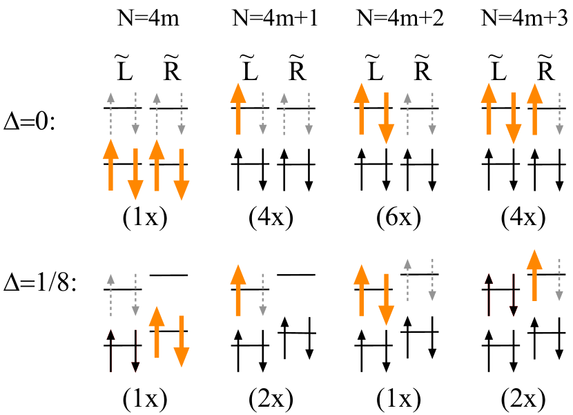
Figure 6: Ground states of the SWNT for different numbers of electrons. For each charge state we show one representative ground state, on top for aligned bands and on the bottom for mismatched bands. In brackets the corresponding degeneracy is given. Full black and orange arrows represent occupied states. The bold (orange) arrows indicate electrons which can contribute to transitions $N\rightarrow N-1$ in the low bias regime. Incoming electrons for the transitions $N\rightarrow N+1$ can be accommodated by the states represented by the dashed arrows. So the number of bold and dashed arrows is equal to $C_{N,N-1}$ and $C_{N,N+1}$ respectively.

We will refer to this kind of master equations as "commonly used master equations" (CMEs). In the low bias regime the occupation probabilities $\rho_{\vec{N}\vec{N}}^{I,E_{M}^{0}}$ of the groundstates containing $M$ particles will all be the same in the stationary solution. Therefore, we introduce the probability for finding the system in charge state $M$ by

$$P_{M}=d_{M}\rho_{\vec{N}\vec{N}}^{I,E_{M}^{0}}(t),$$

where $d_{M}$ is the degeneracy of the corresponding ground states. Using (17), the general expression for the master equation, we find the following CME for $P_{M}$,

$$\frac{\dot{P}_{M}}{d_{M}}=-R_{\vec{N}\vec{N}\vec{N}\vec{N}}^{E_{M}^{0}}\frac{P_{M}}{d_{M}}+\sum_{\vec{N}^{\prime}}R_{\vec{N}\vec{N}\vec{N}^{\prime}\vec{N}^{\prime}}^{E_{M}^{0}E_{M^{\prime}}^{0}}\frac{P_{M^{\prime}}}{d_{M^{\prime}}}.$$ (67)

With equations (18) and (19) for the Redfield tensors we obtain

$$\dot{P}_{M}=-\sum_{l}\left(\Sigma_{l}^{M\rightarrow M^{\prime}}-\Sigma_{l}^{M^{\prime}\rightarrow M}\right)=\\ -2\sum_{l}\sum_{\vec{N}^{\prime}}\left(\Gamma_{l\,\vec{N}\vec{N}^{\prime}}^{E_{M}^{0}E_{M^{\prime}}^{0}}P_{M}-\frac{d_{M}}{d_{M^{\prime}}}\Gamma_{l\,\vec{N}^{\prime}\vec{N}}^{E_{M^{\prime}}^{0}E_{M}^{0}}P_{M^{\prime}}\right),$$ (68)

where we have defined

$$\sum_{\vec{N}^{\prime}}\Gamma_{l,\vec{N}\vec{N}^{\prime}}^{E_{M}^{0}E_{M^{\prime}}^{0}}:=\sum_{\vec{N}^{\prime}}\Gamma_{l\,\vec{N}\vec{N}^{\prime}\vec{N}^{\prime}\vec{N}}^{(+)E_{M}^{0}E_{M^{\prime}}^{0}}.$$ (69)

Using the relation

$$\frac{d_{M}}{d_{M^{\prime}}}\sum_{\vec{N}^{\prime}}\Gamma_{l\,\vec{N}^{\prime}\vec{N}}^{E_{M^{\prime}}^{0}E_{M}^{0}}=\sum_{\vec{N}^{\prime}}\Gamma_{l\,\vec{N}\vec{N}^{\prime}}^{E_{M^{\prime}}^{0}E_{M}^{0}}$$ (70)

the stationary solution of (68) is easily obtained,

$$P_{M}=\frac{\sum_{\vec{N}^{\prime}}\Gamma_{l\,\vec{N}\vec{N}^{\prime}}^{E_{M^{\prime}}^{0}E_{M}^{0}}}{\Gamma_{tot}},$$ (71)

with

$$\Gamma_{tot}=\sum_{l}\sum_{\vec{N}^{\prime}}\left(\Gamma_{l\,\vec{N}\vec{N}^{\prime}}^{E_{N}^{0}E_{N+1}^{0}}+\Gamma_{l\,\vec{N}\vec{N}^{\prime}}^{E_{N+1}^{0}E_{N}^{0}}\right).$$ (72)

The current is obtained from (23). Evaluated at the source for example it yields,

$$I_{N,N+1}=\\ \frac{2e\sum_{\vec{N}^{\prime}}\left(\Gamma_{s\,\vec{N}\vec{N}^{\prime}}^{E_{N}^{0}E_{N+1}^{0}}\Gamma_{d\,\vec{N}\vec{N}^{\prime}}^{E_{N+1}^{0}E_{N}^{0}}-\Gamma_{s\,\vec{N}\vec{N}^{\prime}}^{E_{N+1}^{0}E_{N}^{0}}\Gamma_{d\,\vec{N}\vec{N}^{\prime}}^{E_{N}^{0}E_{N+1}^{0}}\right)}{\Gamma_{tot}}.$$ (73)

The rates $\Gamma_{l,\vec{N}\vec{N}^{\prime}}^{E_{M}^{0}E_{M^{\prime}}^{0}}$ are obtained by using equations (59) and (60),

$$\Gamma_{l\,\vec{N}\vec{N}^{\prime}}^{E_{N}^{0}E_{N+1}^{0}}=\\ \frac{\pi}{\hbar}\Phi_{l}\rho_{l}f(\varepsilon_{l})\sum_{r\sigma}\left(\psi_{r\sigma l}\right)_{\vec{N}\vec{N}^{\prime}}^{E_{N}^{0}\,E_{N+1}^{0}}\left(\psi_{r\sigma l}^{\dagger}\right)_{\vec{N}^{\prime}\vec{N}}^{E_{N+1}^{0}\,E_{N}^{0}},$$

and

$$\Gamma_{l\,\vec{N}\vec{N}^{\prime}}^{E_{N+1}^{0}E_{N}^{0}}=\\ \frac{\pi}{\hbar}\Phi_{l}\rho_{l}\left(1-f(\varepsilon_{l})\right)\sum_{r\sigma}\left(\psi_{r\sigma l}^{\dagger}\right)_{\vec{N}\vec{N}^{\prime}}^{E_{N+1}^{0}\,E_{N}^{0}}\left(\psi_{r\sigma l}\right)_{\vec{N}^{\prime}\vec{N}}^{E_{N}^{0}\,E_{N+1}^{0}}.$$

Here we have assumed that $\Phi_{l}$ and $\rho_{l}$ are constant in the relevant energy range. Furthermore we have defined $\varepsilon_{l}=eV_{l}-\Delta E$ and $\Delta E=E_{N}^{0}-E_{N+1}^{0}.$ From (54) we obtain (remember that $\psi_{\tilde{r}\sigma l}:=\psi_{\tilde{r}\sigma K_{0}}(x_{l})/A(x_{l})$),

$$\sum_{\tilde{r}\sigma}\sum_{\vec{N}^{\prime}}\left(\psi_{r\sigma l}^{\dagger}\right)_{\vec{N}\vec{N}^{\prime}}^{E_{M}^{0}\,E_{M^{\prime}}^{0}}\left(\psi_{r\sigma l}\right)_{\vec{N}^{\prime}\vec{N}}^{E_{M}^{0}\,E_{M^{\prime}}^{0}}=\frac{1}{2L}C_{M,M^{\prime}},$$

where $C_{M,M^{\prime}}$ is the number of ground states with $M^{\prime}$ particles that differ from a given band filling vector $\vec{N}$ for one of the ground state with $M$ particles only by a unit vector (see Fig. 6). Therefore we get

$$2\sum_{\vec{N}^{\prime}}\Gamma_{l\,\vec{N}\vec{N}^{\prime}}^{E_{N}^{0}E_{N+1}^{0}}=\gamma_{l}f(\varepsilon_{l})C_{N,N+1}$$ (74)

as well as

$$2\sum_{\vec{N}^{\prime}}\Gamma_{l\,\vec{N}\vec{N}^{\prime}}^{E_{N+1}^{0}E_{N}^{0}}=\gamma_{l}\left(1-f(\varepsilon_{l})\right)C_{N+1,N},$$ (75)

with $\gamma_{l}=\frac{\pi}{L\hbar}\Phi_{l}\rho_{l}.$ Inserting the rates (74) and (75) into expression (73) for the current results in

$$I_{N,N+1}=e\frac{C_{N,N+1}C_{N+1,N}\gamma_{s}\gamma_{d}\left[f(\varepsilon_{s})-f(\varepsilon_{d})\right]}{\sum_{l}\gamma_{l}\left[f(\varepsilon_{l})C_{N,N+1}+(1-f(\varepsilon_{l}))C_{N+1,N}\right]}.$$ (76)

4.3.1 Linear conductance

In the regime $\left|eV\right|\ll kT\ll\varepsilon_{0}$ we can further simplify (76) by linearising $I_{NN+1}$ in the bias voltage. We choose $-eV_{s}=eV_{d}=:e\frac{V_{b}}{2}$ and obtain

$$I_{N,N+1}=\\ \frac{e^{2}\beta C_{N,N+1}C_{N+1,N}\gamma_{s}\gamma_{d}}{\sum_{l}\gamma_{l}\left(f_{0}C_{N,N+1}+(1-f_{0})C_{N+1,N}\right)}\frac{e^{-\Delta E}}{\left(e^{-\Delta E}+1\right)^{2}}V_{b},$$

with $f_{0}=f(-\Delta E).$ Unlike one could expect, the maxima of the conductance $G_{N,N+1}=I_{N,N+1}/V_{b}$ are not at $\Delta E=0,$ but at

$$\Delta E_{\mathrm{max}}=\frac{1}{2\beta}ln\frac{C_{N+1,N}}{C_{N,N+1}},$$

which is only zero for $C_{N+1,N}=C_{N,N+1}.$ The height of the conductance peaks is

$$G_{N,N+1}^{\mathrm{max}}=\\ \frac{\gamma_{s}\gamma_{d}C_{N,N+1}C_{N+1,N}}{\left(\gamma_{s}+\gamma_{d}\right)\left(C_{N,N+1}+C_{N+1,N}+2\sqrt{C_{N,N+1}C_{N+1,N}}\right)}e^{2}\beta.$$ (77)

We still have to determine the values of $C_{N,N+1}$ and $C_{N+1,N},$ which depend on the mismatch between the $\tilde{R}$ and the $\tilde{L}$ band. If both bands are aligned $(\Delta=0,\,1/2)$ one finds from Fig. 6, $C_{N,N+1}=4,3,2,1$ and $C_{N+1,N}=1,2,3,4$ for $N=4m,\,4m+1,\,4m+2,\,4m+3.$ Then the conductance $G_{N,N+1}$ shows fourfold electron periodicity with two equally high central peaks for $N=4m+1,\,4m+2$ and two smaller ones for $N=4m,\,4m+3$ (cf. Fig. 7 a)). The relative height between central and outer peaks is $G_{4m+1,4m+2}^{\mathrm{max}}/G_{4m,4m+1}^{\mathrm{max}}=27/(10+4\sqrt{6})\approx 1.36.$ Note that this ratio is independent of a possible asymmetry $\gamma_{s}\neq\gamma_{d}$ in the lead contacts. In addition, the conductance is symmetric under an exchange of the sign of the bias voltage.

In the case of an energy mismatch between the $\tilde{R}$ and the $\tilde{L}$ band exceeding well the thermal energy, the degeneracy of the ground states is either $1$ or $2$ and we get $C_{N,N+1}=2,1,2,1$ and $C_{N,N+1}=1,2,1,2$ for $N=4m,\,4m+1,\,4m+2,\,4m+3.$ Therefore, according to (77), all the conductance peaks have the same height as depicted in Fig. 8 a) .

4.3.2 Low bias regime well outside of the Coulomb diamonds

Now we examine the regime where still only ground states are occupied but where we are well outside the region of Coulomb blockade, i.e. $\varepsilon_{0}\gg\left|eV_{l}\pm\Delta E\right|\gg kT.$ Then we have $\left|f(\varepsilon_{s})-f(\varepsilon_{d})\right|=1.$ If e.g. $eV_{s}-\Delta E<0$ and $eV_{d}-\Delta E>0,$ such that electrons tunnel in from the source and tunnel out at the drain, we have $f(\varepsilon_{s})=1$ and $f(\varepsilon_{d})=0$ such that (76) becomes

$$I_{N,N+1}=e\frac{C_{N,N+1}C_{N+1,N}\gamma_{s}\gamma_{d}}{\gamma_{s}C_{N,N+1}+\gamma_{d}C_{N+1,N}}.$$ (78)

The height of the plateaus in the current of Figures 7 b) and 8 b) are described by (78). If the $\tilde{R}$ band is aligned with the $\tilde{L}$ band, we still find a fourfold electron periodicity. But only for $\gamma_{s}=\gamma_{d}$ the pattern with two central peaks and two smaller outer peaks is preserved. The corresponding ratio of the heights is $3/2.$ If $\gamma_{s}\neq\gamma_{d}$ this latter symmetry is lost.

For mismatched bands and $\gamma_{s}=\gamma_{d}$ we find like for the conductance peaks that all current maxima are of the same size. In the case of asymmetric tunnelling contacts, $\gamma_{s}\neq\gamma_{d},$ a pattern of alternating small and large peaks is found.

If we invert the sign of the bias voltage, the current is obtained by flipping its direction and exchanging $\gamma_{s}$ with $\gamma_{d}$ in (78). Then, if $\gamma_{s}\neq\gamma_{d},$ the current does not only change its sign but also changes its magnitude because of $C_{N,N+1}\neq C_{N+1,N}$.

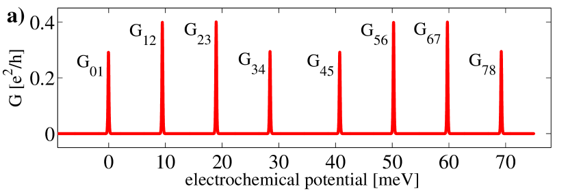
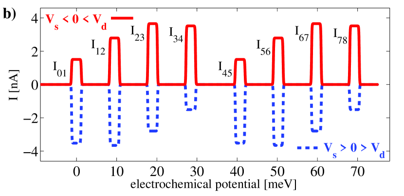
Figure 7: Gate traces for $\Delta=0$, i.e. for aligned $\tilde{R}$ and $\tilde{L}$ bands, at low bias voltage. Parameters are $E_{c}=9.5$ meV, $k_{B}T=0.10$ meV, $\varepsilon_{0}=2.9$ meV and the chosen asymmetry is $\gamma_{s}=5\gamma_{d}=4.9\cdot 10^{10}\textrm{s}^{-1}$. a) Conductance in the linear regime $eV_{b}\ll k_{B}T\ll\varepsilon_{0}.$ Despite asymmetric contacts, we find the repeating pattern of two small outer peaks and two large central peaks. b) Current in the regime $k_{B}T\ll\left|eV_{l}\right|\ll\varepsilon_{0}.$ Asymmetry effects appear. The fourfold periodicity is retained. The upper and lower pattern correspond to opposite values of the bias voltage.

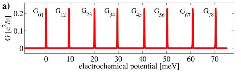
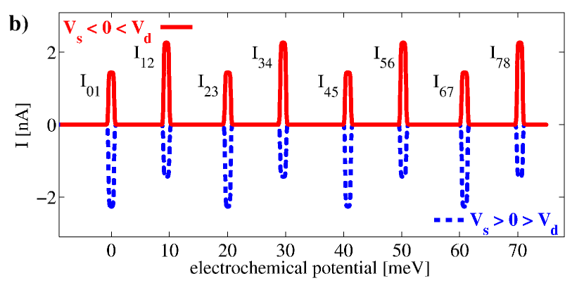
Figure 8: Gate traces for $\Delta=0.2$, i.e. for mismatched $\tilde{R}$ and $\tilde{L}$ bands, at low bias voltage. Other parameters are $E_{c}=9.5$ meV, $k_{B}T=0.10$ meV, $\varepsilon_{0}=2.9$ meV and the chosen asymmetry is $\gamma_{s}=5\gamma_{d}=4.9\cdot 10^{10}\textrm{s}^{-1}$. a) Conductance in the linear regime $eV_{b}\ll k_{B}T\ll\varepsilon_{0}.$ The conductance peaks are all of the same height. b) Current in the regime $k_{B}T\ll\left|eV_{l}\right|\ll\varepsilon_{0}.$ The contact asymmetry leads to alternating large and small current maxima.

4.4 High bias regime

In the bias regime $eV>\varepsilon_{0}$ not only the ground states will contribute to transport but also states with bosonic excitations and band filling configurations $\vec{N}$ different from the ground state configurations. We refer to the latter type of excitations as fermionic excitations. Since the number of relevant states increases rapidly with increasing bias voltage, an analytical treatment is not possible any more and we have to resort to numerical methods in order to calculate the stationary solution of the master equation (17) and the respective current. From (65) we know that at low temperatures the current only changes considerably near the excitation lines given therein. Therefore we can reduce drastically the number of $(eV,\ \mu_{g})$ points for which we actually perform the numerical calculations, saving computing time. In Figs. 9 a) and 10, the current as a function of the applied bias voltage and the electrochemical potential in the dot is depicted. The chosen parameters for $E_{c},\,\varepsilon_{0}$ and $\Delta$ are the ones we have obtained for fitting the data of sample C and sample A of Sapmaz2005 , respectively. Hence Figs. 9 and 10 show the current for SWNTs with the $\tilde{R}$ and $\tilde{L}$ band being aligned ($\Delta=0$) and mismatched ($\Delta\approx 0.17$). In both cases a symmetric coupling to the leads, i.e. $\gamma_{s}=\gamma_{d},$ is assumed. In the transport calculations the lowest lying $c+$ excitations are taken into account using $g=0.21$ for the Luttinger parameter (cf. equation (50) for the definition of $g$).

In addition we have also determined the current using the CME, hence ignoring any coherences in the RDM. For the current corresponding to Fig. 9, the quantitative difference between the calculations with and without coherences is considerable in the region of intermediate bias voltage as we show in Fig. 9 b). On the other hand the deviation of the CME result from the calculation including coherences is by far less pronounced for the parameter choice of Fig. 10. The crucial point here is that the charging energy $E_{c}$ is smaller than $\varepsilon_{0}$, the level spacing of the neutral system. Then the subsequent considerations are not strictly valid. Now we explain why coherences can’t be generally ignored if considering interacting electrons in a SWNT.

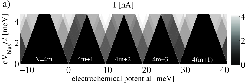
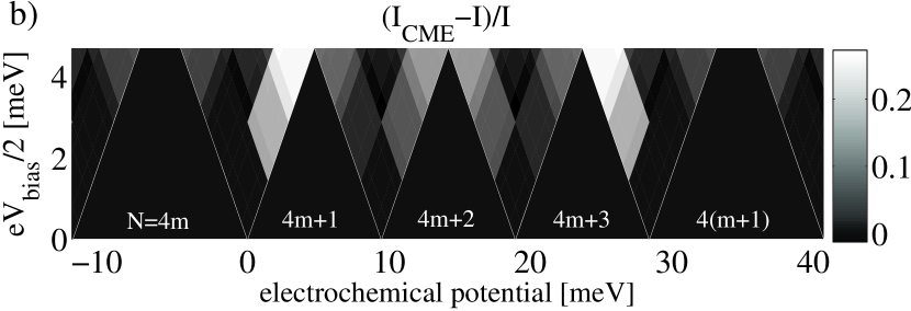
Figure 9: a) Current in a bias voltage - electrochemical potential plane for the symmetric contacts case. b) Difference plot of the current with and without coherences. Here $k_{B}T=0.01\,\mathrm{meV}$ and the interaction parameter is $g\approx 0.21$. Other parameters are as for Fig. 7.

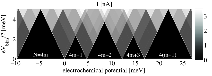
Figure 10: Current as a function of the bias voltage and the electrochemical potential in the SWNT for symmetric contacts. The parameters here are chosen to fit the positions of the Coulomb diamonds of sample A in Sapmaz2005 , i.e. $E_{c}=4.7$ meV, $2\Delta\varepsilon_{0}=2.8$ meV, $\varepsilon_{0}=8.2$ meV.

4.4.1 Why and when are coherences needed?

As in the low bias regime we assume to have unpolarized leads, i.e. we use condition (62), such that we can ignore coherences between states with different fermionic configurations $\vec{N}$. Unlike in the low bias regime, we are not only left with diagonal elements of the RDM but there still might be coherences between degenerate states which have the same $\vec{N}$ but different bosonic excitations $\vec{m}.$ For the importance of these kind of coherences it is illuminating to discuss our system without electron-electron interactions, i.e. for the moment let us assume that an eigenbasis of $H_{\odot}$ is given by the Slater determinants of the single electron states $\left|\varphi_{\tilde{r}\kappa}^{OBC}\right\rangle\left|\sigma\right\rangle.$ Furthermore, we concentrate without loss of generality on the case $\Delta=0$, and we assume that the charging energy $E_{c}$ exceeds $\varepsilon_{0}$. Each of the Slater determinants can be denoted by the occupation $\vec{n}$ of the single electron states. In the case condition (62) holds, it is again easy to show that coherences vanish in the stationary solution of the master equation (17), if the RDM is expressed in the $\left|\vec{n}\right\rangle$ basis. But of course we still could use the states $\left|\vec{N},\vec{m}\right\rangle$ from (51) as eigenbasis, now with four neutral modes $c+,c-,s+,s-.$ In the $\left|\vec{N},\vec{m}\right\rangle$ basis it is crucial to include the off diagonal elements in order to get the right stationary solution as we show in the following example.

We adjust the voltages such that only transitions are possible from the ground state with $4m$ particles and energy $E_{4m}^{0}$ to ground and first excited states with $4m+1$ particles and energies $E_{4m+1}^{0}$ and $E_{4m+1}^{1}=E_{4m+1}^{0}+\varepsilon_{0}$, respectively. From the $4m+1$ ground states only transitions to the $4m$ ground state shall be allowed as depicted in Fig. 11 a). Note that this situation is only stable, because we have made the choice $E_{c}>\varepsilon_{0}$. The master equation expressed in the $\left|\vec{n}\right\rangle$ basis reveals that only four of the 16 states with the lowest particle hole excitation are indeed occupied in the stationary limit (cf. side b) of Fig. 11, because not all of the corresponding energetically allowed transitions from the $N=4m$ ground state can be mediated by one-electron tunnelling processes.

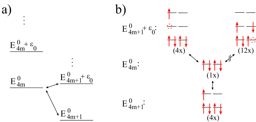
Figure 11: a) Scheme of relevant energy levels, if transitions from the ground state with $N=4m$ particles to the first excited state with $N=4m+1$ particles are energetically allowed, while no transitions from the $N=4m+1$ ground states to excited states with $N=4m$ electrons are possible. b) Possible transitions between the $N=4m$ and $N=4m+1$ electron states of the noninteracting system, which are energetically allowed in situation a). The degeneracy of the eigenstates is given in brackets.

Whereas in the $\left|\vec{N},\vec{m}\right\rangle$ basis, all 16 states with the energetically lowest bosonic excitations are equally populated. Since the degenerate states of the two bases are connected by a unitary transformation, the same must be true for the corresponding matrix representations of $\rho_{\odot}^{I,E_{4m+1}^{1}}.$ From the representation of the RDM in the $\left|\vec{n}\right\rangle$ basis, we know that the rank of $\rho_{\odot}^{I,E_{4m+1}^{1}}$ must be equal to $4$. Because an unitary transformation does not change the rank of a matrix, the stationary solution in the $\left|\vec{N},\vec{m}\right\rangle$ basis can maximally have 4 linearly independent columns. Since all diagonal elements are nonvanishing this is only possible if there are also nonvanishing coherences.

Switching on the electron - electron interactions, the $\left|\vec{n}\right\rangle$ states are no longer an eigenbasis of the SWNT Hamiltonian and hence we must work in the $\left|\vec{N},\vec{m}\right\rangle$ basis. But then, as we know from the discussion above, the coherences are expected to be of importance.

4.4.2 Negative differential conductance

Spin charge separation and therefore non-Fermi liquid behavior could also manifest itself in the occurrence of negative differential conductance (NDC) at certain excitation lines involving transitions to states with fermionic excitations, as was predicted for a spinful Luttinger liquid quantum dot Cavaliere2004 with asymmetric contacts. We also find this effect for the nonequilibrium treatment of the SWNT quantum dot. Since in our case only the energy spectrum of the $c+$ mode depends on the interaction and the other three modes have the same energies as the neutral system, rather large asymmetries are needed in order to observe NDC. In Fig. 12 we show the current across the first excitation line for transitions from $N=4m+1$ to $N=4m$ in the $\Delta=0$ case. The corresponding trace in the $\mu_{b}$-$V_{b}$ plane is indicated in the inset of Fig. 12 a). Here the origin of the NDC is that some states with fermionic excitations have lower transition rates than nonexcited states, since due to the increased energy of the $c+$ modes less channels are available for transport. In Fig. 12 b) we show some of the excited states with $N=4m$ electrons which are responsible for the NDC, because their transition amplitudes to states with $N=4m+1$ electrons are reduced compared with the one of the $4m$ ground state. Apart from the asymmetries all other parameters are chosen as for Fig. 9. Only for asymmetries $a=\gamma_{d}/\gamma_{s}$ larger than around $45$, clear NDC features are seen.

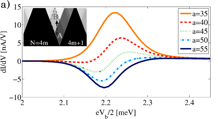
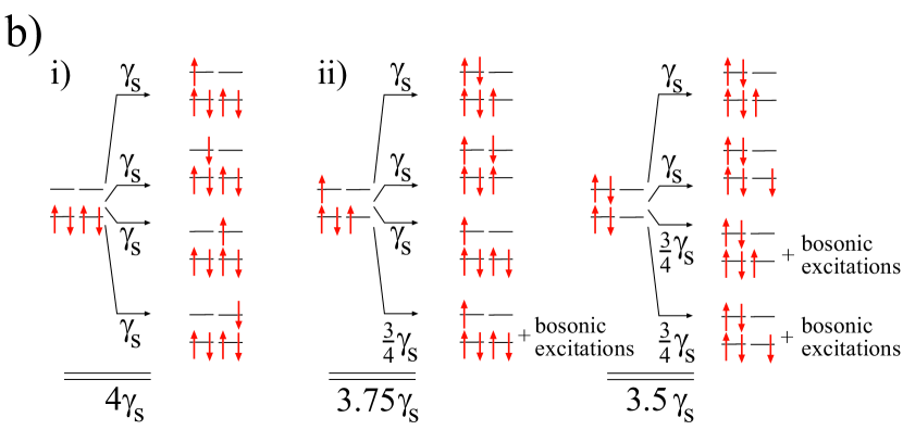
Figure 12: a) Differential conductance as a function of the bias voltage for different asymmetries $a=\gamma_{d}/\gamma_{s}$ of the coupling to the leads. The trace in the $\mu_{b}$-$V_{b}$ plane across the boundary between regions A and B is indicated in the inset. Only for asymmetries larger than around $45$ negative differential conductance occurs. All parameters here are chosen as for Fig. 9, except for $k_{B}T$ a value of $0.026$ meV was used. b) The transitions responsible for NDC. i) In region A of the inset from a) only transitions between ground states are possible at low enough temperature. The transition rate from the $N=4m$ ground state to the $N=4m+1$ ground states is given by $4\gamma_{s}$ (see equation (74)). ii) In region B additionally excited states become occupied. For some of the states with $N=4m$ electrons and fermionic excitations the transition rates to states with $N=4m+1$ electrons and neutral bosonic excitations is decreased compared to the ground state rate as a consequence of the larger energies of $c+$ excitations, which are not available for transport yet. Notice that we only show the most important types of transitions from $N=4m$ to $N=4m+1$ that take place in region B. Since we are considering a nonequilibrium situation other types of transitions are possible in principle.

5 Conclusions

In this article we have analyzed the linear and nonlinear current as a function of the gate and bias voltage across metallic SWNT quantum dots. The properties of the SWNT itself were derived from a microscopic model including electron - electron interactions. Exchange and related effects, which become relevant for small diameter SWNTs, have not been taken into account. The energy spectrum of a metallic SWNT, which can be obtained with the help of bosonization, turned out to be highly degenerate as a consequence of both fermionic and bosonic excitations. In the linear bias regime, the degeneracy of the groundstates leads to a characteristic pattern of conductance peaks depending on whether the two branches of the dispersion relation are aligned or not. Leaving the linear regime, asymmetry effects become relevant. Thus measurements of the current at low bias voltages, in the linear and nonlinear regime, in principle allow the separate determination of the source and drain tunnelling resistances as a function of the gate voltage. At higher bias voltages also excited states become relevant. The correct calculation of the nonequilibrium dynamics of the system then requires the inclusion of coherences in the reduced density matrix between degenerate states with bosonic excitations. At intermediate bias voltages there is a considerable deviation between the transport calculations with and without coherences. We emphasize that for a noninteracting system with unpolarized leads, coherences do not have to be considered if expressing the reduced density matrix in terms of Slater determinants, formed by the one electron wave functions of the noninteracting system. Another consequence of the electron correlations is the formation of a non-oscillatory spatial dependence of the tunnelling amplitudes along the nanotube axis. For transitions between states with energetically low excitations we find a strong suppression of the tunnelling amplitudes near the SWNT ends. Furthermore we have addressed the influence of the tunnelling contacts on the transport. We have shown that extended contacts described as 3D Fermi gas do not lead to a polarization of the contacts with respect to the two branches of the dispersion relation. We think that a further investigation of this point for other types of contacts is worthwhile.

***

Useful discussions with S. Sapmaz and support by the DFG under the program GRK 638 are acknowledged.

Appendix A Description of the tunnelling contacts

In this appendix we discuss the dependence of the rates $\Gamma_{l,k^{\prime}mnk}^{(\alpha)E_{M}\,E_{M^{\prime}}}$ on the properties of the tunnelling contacts. In Section 4 we have introduced the parameters $\Phi_{lrr^{\prime}}(\varepsilon)$ with equation (58). Here we show the calculation of these parameters assuming a 3D electron gas in the leads. Furthermore, we require that the tunnelling region extends over several sites of the SWNT lattice. Starting from (20) together with (16) and (33) we can characterize the part of $\Gamma_{l,k^{\prime}mnk}^{(\alpha)E_{N}\,E^{\prime}_{N+1}}$ that depends on the tunnelling contact $l$ by the following expression,

$$\mathcal{T}_{l,nkk^{\prime}m}(\varepsilon):=\sum_{FF^{\prime}}\mathrm{sgn}(FF^{\prime})\int d^{3}r\int d^{3}r^{\prime}T_{l}^{*}(\vec{r})T_{l}(\vec{r}^{\prime})\times\\ \sum_{\vec{q}|_{\varepsilon}}\phi_{l\vec{q}}^{*}(\vec{r})\phi_{l\vec{q}}(\vec{r}^{\prime})\sum_{\tilde{r}\tilde{r}^{\prime}\sigma}\tilde{\varphi}_{\mathrm{sgn}(F)\tilde{r}\,F}(\vec{r})\tilde{\varphi}_{\mathrm{sgn}(F^{\prime})\tilde{r}^{\prime}\,F^{\prime}}^{*}(\vec{r}^{\prime})\times\\ \left(\psi_{\tilde{r}F\sigma}(x)\right)_{nk}\left(\psi_{\tilde{r}^{\prime}F^{\prime}\sigma}^{\dagger}(x^{\prime})\right)_{k^{\prime}m}.$$ (79)

The wave functions in the leads are denoted $\phi_{l\vec{q}}$ and the sum $\sum_{\vec{q}|_{\varepsilon}}$ extends over all $\vec{q}$ values that correspond to the energy $\varepsilon.$ At low enough energies, oscillations of the product $\left(\psi_{\tilde{r}F\sigma}(x)\right)_{nk}\left(\psi_{\tilde{r}^{\prime}F^{\prime}\sigma}^{\dagger}(y)\right)_{k^{\prime}m}$ can be ignored along the length of the tunnelling interfaces. Using (54) we thus can rewrite (79) as

$$\mathcal{T}_{l,nkk^{\prime}m}(\varepsilon)=L\sum_{FF^{\prime}}\mathrm{sgn}(FF^{\prime})\nu_{lFF^{\prime}}(\Delta)\times\\ \int d^{3}r\int d^{3}r^{\prime}T_{l}^{*}(\vec{r})T_{l}(\vec{r}^{\prime})A(x)A(x^{\prime})\sum_{\vec{q}|_{\varepsilon}}\phi_{l\vec{q}}^{*}(\vec{r})\phi_{l\vec{q}}(r^{\prime})\times\\ \sum_{\tilde{r}\tilde{r}^{\prime}\sigma}\varphi_{\mathrm{sgn}(F)\tilde{r}\,F}(\vec{r})\varphi_{\mathrm{sgn}(F^{\prime})\tilde{r}^{\prime}\,F^{\prime}}^{*}(\vec{r}^{\prime})\left(\psi_{\tilde{r}\sigma l}\right)_{nk}\left(\psi_{\tilde{r}^{\prime}\sigma l}^{\dagger}\right)_{k^{\prime}m}.$$ (80)

Here the factor $\nu_{lFF^{\prime}}(\Delta)=e^{i\delta_{l,d}\pi\mathrm{sgn}(F-F^{\prime})\Delta}$ takes into account a possible phase shift due to the band mismatch $\Delta$ and we have used the notation $\psi_{\tilde{r}\sigma l}=\psi_{\tilde{r}K_{0}\sigma}(x_{l})/A(x_{l}),$ where $x_{l}=0,\,L$ for $l=s,\,d.$ Now the parameters $\Phi_{l\tilde{r}\tilde{r}^{\prime}}(\varepsilon)$ from (58) are recovered by the relation

$$\mathcal{T}_{l,nkk^{\prime}m}(\varepsilon)=\sum_{\tilde{r}\tilde{r}^{\prime}}\Phi_{l\tilde{r}\tilde{r}^{\prime}}(\varepsilon)\sum_{\sigma}\left(\psi_{\tilde{r}\sigma l}\right)_{nk}\left(\psi_{\tilde{r}^{\prime}\sigma l}^{\dagger}\right)_{k^{\prime}m}.$$

In the next step we exploit that the Bloch waves $\varphi_{\mathrm{sgn}(F)r\,F}$ from equation (28) are only nonvanishing around the positions of the carbon atoms in the SWNT lattice. On the length scale of the extension of the $p_{z}$ orbitals all other quantities in $\Phi_{l\tilde{r}\tilde{r}^{\prime}}$ are slowly varying. Hence we can rewrite the integrals over $\vec{x}$ and $\vec{y}$ as a sum over the positions of the carbon atoms

$$\Phi_{l\tilde{r}\tilde{r}^{\prime}}(\varepsilon)=C\frac{L}{N_{L}}\sum_{FF^{\prime}}\mathrm{sgn}(FF^{\prime})\nu_{lFF^{\prime}}(\Delta)\times\\ \sum_{p,p^{\prime}}f_{p\mathrm{sgn}(F)r\,F}f_{p^{\prime}\mathrm{sgn}(F^{\prime})r^{\prime}\,F^{\prime}}^{*}\sum_{\vec{R},\vec{R}^{\prime}}T_{l}^{*}(\vec{x}_{\vec{R},p})T_{l}(\vec{x}_{\vec{R}^{\prime},p^{\prime}})\times\\ A(\vec{R}_{x})A(\vec{R}^{\prime}_{x})\sum_{\vec{q}|_{\varepsilon}}\phi_{l\vec{q}}^{*}(\vec{x}_{\vec{R},p})\phi_{l\vec{q}}(\vec{x}_{\vec{R}^{\prime},p^{\prime}})e^{iF\vec{R}}e^{-iF\vec{R}^{\prime}},$$ (81)

where we have defined $\vec{x}_{\vec{R},p}:=\vec{R}+\vec{\tau}_{p}.$ The constant $C$ results from the integration over the $p_{z}$ orbitals. For the 3D electron gas the wave functions $\phi_{l\vec{q}}(\vec{x})$ are simply given by plane waves,

$$\phi_{l\vec{q}}(\vec{x})=\frac{1}{\sqrt{V_{l}}}e^{i\vec{q}\vec{x}}.$$

Therefore we can easily perform the sum over the wave numbers $\vec{q}$ associated with the energy $\varepsilon$,

$$\sum_{\vec{q}|_{\varepsilon}}\phi_{l\vec{q}}^{*}(\vec{x})\phi_{l\vec{q}}(\vec{y})\approx\\ \int_{0}^{2\pi}d\varphi\int_{-1}^{1}d\cos\theta e^{iq|_{\varepsilon}\left|\vec{x}-\vec{y}\right|\cos\vec{\theta}}=\frac{4\pi\sin(q|_{\varepsilon}\left|\vec{x}-\vec{y}\right|)}{q|_{\varepsilon}\left|\vec{x}-\vec{y}\right|}.$$

The previous expression is peaked around $\vec{x}=\vec{y}.$ For $q|_{\varepsilon}>1/\left|\vec{x}-\vec{y}\right|$ the correlations between $\vec{x}$ and $\vec{y}$ drop off fast. It means that if $q|_{\varepsilon}$ is larger than $1/a_{0},$ where $a_{0}$ is the nearest neighbor distance on the SWNT lattice, correlations between different carbon atom sites are suppressed such that we arrive at the following approximation:

$$\sum_{\vec{q}|_{\varepsilon}}\phi_{l\vec{q}}^{*}(\vec{x}_{\vec{R},p})\phi_{l\vec{q}}(\vec{x}_{\vec{R}^{\prime},p^{\prime}})\approx 4\pi\delta_{\vec{R},\vec{R}^{\prime}}\delta_{p,p^{\prime}},$$

which yields

$$\Phi_{l\tilde{r}\tilde{r}^{\prime}}(\varepsilon)=4\pi C\frac{L}{N_{L}}\times\\ \sum_{FF^{\prime}}sgn(FF^{\prime})\nu_{lFF^{\prime}}(\Delta)\sum_{p}f_{p\mathrm{sgn}(F)r\,F}f_{p\mathrm{sgn}(F^{\prime})r^{\prime}\,F^{\prime}}^{*}\times\\ \sum_{\vec{R}}\left|T_{l}(\vec{x}_{\vec{R},p})\right|^{2}e^{i\left(F-F^{\prime}\right)\vec{R}}A^{2}(\vec{R}_{x}).$$ (82)

Since we assume an extended tunnelling region, the fast oscillating terms with $F=-F^{\prime}$ are supposed to cancel. Furthermore we assume that both sublattices are equally well coupled to the contacts, such that the sum over $\vec{R}$ in (82) should approximately give the same result for $p=1$ and $p=2.$ Hence we can separate the sum over $p$ from the rest. Since the Bloch waves $\tilde{\varphi}_{\mathrm{sgn}(F)r\,F}$ and $\tilde{\varphi}_{\mathrm{sgn}(F)r^{\prime}\,F}$ are orthogonal to each other for $r\neq r^{\prime}$, the relation

$$\sum_{p}f_{p\mathrm{sgn}(F)r\,F}f_{p\mathrm{sgn}(F)r^{\prime}\,F}^{*}=\delta_{rr^{\prime}}$$

must hold, as it can be deduced from the explicit expression for the Bloch wave, equation (28), and we arrive at

$$\Phi_{l\tilde{r}\tilde{r}^{\prime}}(\varepsilon)=\delta_{rr^{\prime}}4\pi C\frac{L}{N_{L}}\sum_{\vec{R}}\left|T_{l}(\vec{x}_{\vec{R},p})\right|^{2}A^{2}(\vec{R}_{x}).$$ (83)

We should mention that the treatment of the contact geometry here relies on several assumptions that might not be fulfilled under all circumstances and so it should be seen as a first estimate. For example we assume that the transmission functions $T_{l}$ do not depend on the $\vec{q}$ vector of the incoming wave. But such a dependence would increase the correlation between different atom sites. Furthermore $q|_{\varepsilon}$ will not be much larger than $1/a_{0}$ for all kind of contacts (for gold the Fermi wave number is about $1.5/a_{0}),$ nor can the lead electrons always be described by a 3D electron gas.

Here we want to emphasize, the tunnelling contacts itself play an important role for transport through a SWNT quantum dot. Especially it will be interesting for which kind of contacts the condition

$$\Phi_{l\tilde{r}\tilde{r}^{\prime}}(\varepsilon)\neq\delta_{\tilde{r}\tilde{r}^{\prime}}\Phi_{l}(\varepsilon),$$

of having leads polarized with respect to the band degree of freedom $\tilde{r}$, might be fulfilled.

Appendix B The matrix elements of the electron operators

In this appendix we calculate the expressions for the matrix elements $\left\langle\vec{N},\vec{m}\right|\psi_{\tilde{r}\sigma F}(x)\left|\vec{N}^{\prime},\vec{m}^{\prime}\right\rangle$ using the bosonization identity (52) of the electron operators $\psi_{\tilde{r}\sigma F}(x),$ namely

$$\psi_{\tilde{r}\sigma F}(x)=\frac{\eta_{\tilde{r}\sigma}K_{\tilde{r}F\mathcal{N}_{\tilde{r}\sigma}}}{\sqrt{1-e^{-\alpha\frac{\pi}{L}}}}e^{i\phi_{\tilde{r}\sigma F}^{\dagger}(x)+i\phi_{\tilde{r}\sigma F}(x)}.$$ (84)

As a reminder, $\eta_{r\sigma}$ is the Klein factor reducing the electron number by one, the operator $K_{\tilde{r}F\mathcal{N}_{\tilde{r}\sigma}}$ is given by

$$K_{\tilde{r}F\mathcal{N}_{r\sigma}}(x):=\frac{1}{\sqrt{2L}}e^{i\frac{\pi}{L}\textrm{sgn}F(\textrm{sgn}\tilde{r}\cdot\mathcal{N}_{\tilde{r}\sigma}+\delta)x}$$ (85)

and yields a phase factor depending on the filling of the band $(\tilde{r}\sigma).$ The bosonic fields $\phi_{\tilde{r}F\sigma}(x)$ are given in terms of the bosonic annihilation operators $b_{\sigma q}$,

$$i\phi_{\tilde{r}\sigma F}(x)=\sum_{q>0}\frac{e^{i\textrm{sgn}(F\tilde{r})qx-\alpha q/2}}{\sqrt{n_{q}}}b_{\sigma\textrm{sgn}(\tilde{r})q}.$$ (86)

The action of $\psi_{rF\sigma}(x)$ on the states $\left|\vec{N},\vec{m}\right\rangle$ is conveniently determined by rewriting the operators $b_{\sigma\textrm{sgn}(r)q}$ in terms of the operators $a_{j\delta q}$ and $a_{j\delta q}^{\dagger}$which diagonalize the SWNT Hamiltonian $H_{\odot}$. As we know from the Bogoliubov transformation, the $b$ operators depend linearly on the $a$ operators and hence we can write in general

$$i\phi_{\tilde{r}\sigma F}^{\dagger}(x)+i\phi_{\tilde{r}\sigma F}(x)=\\ =\sum_{q>0}e^{-\alpha q/2}\sum_{j\delta}\left(\lambda_{\tilde{r}\sigma F}^{j\delta q}(x)a_{j\delta q}+\lambda_{\tilde{r}\sigma F}^{\oplus j\delta q}(x)a_{j\delta q}^{\dagger}\right),$$ (87)

where $\lambda_{\tilde{r}\sigma F}^{\oplus j\delta q}(x)=-\left(\lambda_{\tilde{r}\sigma F}^{j\delta q}(x)\right)^{*},$ since $i\phi_{\tilde{r}\sigma F}^{\dagger}(x)+i\phi_{\tilde{r}\sigma F}(x)$ is anti-hermitian. The actual values of the $\lambda$s are calculated below in this appendix. Plugging the bosonization identity (84) together with (87) into $\left\langle\vec{N},\vec{m}\right|\psi_{\tilde{r}\sigma F}(x)\left|\vec{N}^{\prime},\vec{m}^{\prime}\right\rangle$, yields

$$\left\langle\vec{N},\vec{m}\right|\psi_{\tilde{r}\sigma F}(x)\left|\vec{N}^{\prime},\vec{m}^{\prime}\right\rangle=\\ \delta_{\vec{N}+\vec{e}_{\tilde{r}\sigma},\vec{N}^{\prime}}\frac{(-1)^{\sum_{j=1}^{\tilde{r}\sigma-1}N_{j}}}{\sqrt{1-e^{-\alpha\frac{\pi}{L}}}}K_{\tilde{r}F(\vec{N}^{\prime})_{\tilde{r}\sigma}}(x)\times\\ \left\langle\vec{m}\right|e^{\sum_{q>0}e^{-\alpha q/2}\sum_{j\delta}\left(\lambda_{\tilde{r}\sigma F}^{j\delta q}(x)a_{j\delta q}+\lambda_{\tilde{r}\sigma F}^{\oplus j\delta q}(x)a_{j\delta q}^{\dagger}\right)}\left|\vec{m}^{\prime}\right\rangle.$$

Remember that the factor $(-1)^{\sum_{j=1}^{\tilde{r}\sigma-1}N_{j}}$ stems from the Klein factor. The term

$$\left\langle\vec{m}\right|e^{\sum_{q>0}e^{-\alpha q/2}\sum_{j\delta}\left(\lambda_{\tilde{r}\sigma F}^{j\delta q}(x)a_{j\delta q}+\lambda_{\tilde{r}\sigma F}^{\oplus j\delta q}(x)a_{j\delta q}^{\dagger}\right)}\left|\vec{m}^{\prime}\right\rangle$$ (88)

does not depend on the fermionic configuration and therefore we have dropped the $\vec{N}$ index in $\left|\vec{N},\vec{m}\right\rangle$. Now we exploit that in our finite size SWNTs there will always be only a finite number of bosonic excitations. Hence, by using the Baker-Hausdorff formula, $e^{A+B}=e^{A}e^{B}e^{-[A,B]/2}$, we commute all annihilation operators $a_{j\sigma q}$ to the right and all creation operators $a_{j\delta q}^{\dagger}$ to the left in (88):

$$\left\langle\vec{m}\right|e^{\sum_{q>0}e^{-\alpha q/2}\sum_{j\delta}\left(\lambda_{\tilde{r}\sigma F}^{j\delta q}(x)a_{j\delta q}+\lambda_{\tilde{r}\sigma F}^{\oplus j\delta q}(x)a_{j\delta q}^{\dagger}\right)}\left|\vec{m}^{\prime}\right\rangle=\\ e^{-\frac{1}{2}\sum_{q>0}e^{-\alpha q}\sum_{j\delta}\left|\lambda_{\tilde{r}\sigma F}^{j\delta q}(x)\right|^{2}}\times\\ \prod_{q>0}\prod_{j\delta}\left\langle m_{j\delta q}\right|e^{\lambda_{\tilde{r}\sigma F}^{\oplus j\delta q}(x)a_{j\delta q}^{\dagger}}e^{\lambda_{\tilde{r}\sigma F}^{j\delta q}(x)a_{j\delta q}}\left|m^{\prime}_{j\delta q}\right\rangle,$$ (89)

with $\left|m_{j\delta\kappa}\right\rangle=\left(m_{j\delta\kappa}!\right)^{-1/2}\left(a_{j\delta\kappa}^{\dagger}\right)^{m_{j\delta\kappa}}\left|0\right\rangle.$ Expanding the exponentials $e^{\lambda_{\tilde{r}\sigma F}^{j\delta q}(x)a_{j\delta q}}$ in (89), all terms which are of higher order than $m^{\prime}_{j\delta q}$ will vanish. Analogously, all terms in the expansion of $e^{\lambda_{\tilde{r}\sigma F}^{\oplus j\delta q}(x)a_{j\delta q}^{\dagger}}$ of higher order than $m_{j\delta q}$ can be ignored. Hence we get

$$\left\langle m\right|e^{\lambda^{\oplus}a^{\dagger}}e^{\lambda a}\left|m^{\prime}\right\rangle=:F(\lambda,m,m^{\prime})=\\ \left\langle m\left|\sum_{i=0}^{m}\frac{\left(\lambda^{\oplus}a^{\dagger}\right)^{i}}{i!}\sum_{j=0}^{m^{\prime}}\frac{\left(\lambda a\right)^{j}}{j!}\right|m^{\prime}\right\rangle.$$ (90)

Here, in favor of readability all indices have been dropped. In (90) only the terms with $m-i=m^{\prime}-j$ survive. For $m^{\prime}>m$ we conveniently express $j$ in terms of $i$ and get:

$$F(\lambda,m,m^{\prime})=\lambda^{m^{\prime}-m}\sqrt{\frac{m!}{m^{\prime}!}}\sum_{i=0}^{m}\frac{\left(\lambda^{\oplus}\lambda\right)^{i}}{i!(i+m^{\prime}-m)!}\frac{m^{\prime}!}{(m-i)!}$$ (91)

and for $m^{\prime}<m$ we write $i$ in terms of $j$ and get

$$F(\lambda,m,m^{\prime})=\\ \underbrace{\left(\lambda^{\oplus}\right)^{m-m^{\prime}}}_{\left(-\lambda^{*}\right)^{m-m^{\prime}}}\sqrt{\frac{m^{\prime}!}{m!}}\sum_{j=0}^{m^{\prime}}\frac{\left(\lambda^{\oplus}\lambda\right)^{j}}{j!(j+m-m^{\prime})!}\frac{m!}{(m^{\prime}-j)!}.$$ (92)

Defining $m_{\mathrm{max}/\mathrm{min}}:=\max\textrm{/}\min(m,m^{\prime})$, we can summarize (91) and (92) as

$$F(\lambda,m,m^{\prime})=\\ =\left(\Theta(m^{\prime}-m)\lambda^{m^{\prime}-m}+\Theta(m-m^{\prime})\left(-\lambda^{*}\right)^{m-m^{\prime}}\right)\\ \times\sqrt{\frac{m_{\mathrm{min}}!}{m_{\mathrm{max}}!}}\sum_{i=0}^{m_{\mathrm{min}}}\frac{\left(-\left|\lambda\right|^{2}\right)^{i}}{i!(i+m_{\mathrm{max}}-m_{\mathrm{min}})!}\frac{m_{\mathrm{max}}!}{(m_{\mathrm{min}}-i)!},$$ (93)

or in terms of the Laguerre polynomials gradshteyn2000 ,

$$F(\lambda,m,m^{\prime})=\sqrt{\frac{m_{\mathrm{min}}!}{m_{\mathrm{max}}!}}L_{m_{\mathrm{min}}}^{m_{\mathrm{max}}-m_{\mathrm{min}}}(\left|\lambda\right|^{2})\times\\ \left(\Theta(m^{\prime}-m)\lambda^{m^{\prime}-m}+\Theta(m-m^{\prime})\left(-\lambda^{*}\right)^{m-m^{\prime}}\right).$$ (94)

Similar expressions for $F(\lambda,m,m^{\prime})$ were found by Kim et al. Kim2003 when investigating charge plasmons in a spinless Luttinger liquid quantum dot. In the end we obtain for the matrix elements $\left(\psi_{\tilde{r}\sigma F}(x)\right)_{nm}$ the following expression:

$$\left\langle\vec{N},\vec{m}\right|\psi_{\tilde{r}\sigma F}(x)\left|\vec{N}^{\prime},\vec{m}^{\prime}\right\rangle=\\ \delta_{\vec{N}+\vec{e}_{\tilde{r}\sigma}\vec{N}^{\prime}}(-1)^{\sum_{j=1}^{\tilde{r}\sigma-1}N_{j}}K_{\tilde{r}F(\vec{N}^{\prime})_{\tilde{r}\sigma}}(x)A(x)\times\\ \prod_{q>0}\prod_{j\delta}F(\lambda_{\tilde{r}\sigma F}^{j\delta q}(x),m_{j\delta q},m^{\prime}_{j\delta q}),$$

where we have defined

$$A(x):=\frac{e^{-\frac{1}{2}\sum_{q>0}e^{-\alpha q}\sum_{j\delta}\left|\lambda_{\tilde{r}\sigma F}^{j\delta q}(x)\right|^{2}}}{\sqrt{1-e^{-\alpha\frac{\pi}{L}}}}.$$

Appendix C The parameters $\lambda$

We still have to determine the values of the parameters $\lambda_{r\sigma F}^{j\delta q}(x)$ for our case. Using equation (86) we can express the sum $i\phi_{r\sigma F}^{\dagger}(x)+i\phi_{r\sigma F}(x)$ in terms of the bosonic operators $b_{\sigma q},$

$$i\phi_{r\sigma F}^{\dagger}(x)+i\phi_{r\sigma F}(x)=\sum_{q>0}\frac{e^{-\alpha q/2}}{\sqrt{n_{q}}}\times\\ \left(-e^{-i\textrm{sgn}(Fr)qx}b_{\sigma\textrm{sgn}(r)q}^{\dagger}+e^{i\textrm{sgn}(Fr)qx}b_{\sigma\textrm{sgn}(r)q}\right),$$ (95)

which in turn are related to the operators $a_{j\delta q}$ and $a_{j\delta q}^{\dagger}$ via equation (45). Hence

$$i\phi_{r\sigma F}^{\dagger}(x)+i\phi_{r\sigma F}(x)=\\ \sum_{j\delta}\Lambda_{\sigma\tilde{r}}^{j\delta}\sum_{q>0}\frac{e^{-\alpha q/2}}{\sqrt{n_{q}}}\left[e^{i\textrm{sgn}(Fr)qx}\left(C_{j\delta q}a_{j\delta q}^{\dagger}+S_{j\delta q}a_{j\delta q}\right)\right.\\ \left.-e^{-i\textrm{sgn}(Fr)qx}\left(S_{j\delta q}a_{j\delta q}^{\dagger}+C_{j\delta q}a_{j\delta q}\right)\right]$$ (96)

By comparing (96) to (87) the values of the $\lambda$s can be read off:

$$\lambda_{\tilde{r}\sigma F}^{j\delta q}(x)=\\ \frac{1}{\sqrt{n_{q}}}\Lambda_{\tilde{r}\sigma}^{j\delta}\left(-e^{-i\textrm{sgn}(Fr)qx}C_{j\delta q}+e^{i\textrm{sgn}(Fr)qx}S_{j\delta q}\right).$$

With the coefficients $C_{j\delta q},\,S_{j\delta q}$ and $\Lambda_{\sigma\tilde{r}}^{j\delta}$ from (46), (47) and (48) we get for $j\delta=c-,s+,s-,$

$$\lambda_{\tilde{r}\sigma F}^{j\delta q}(x)=\frac{e^{i\mathrm{sgn}(F\tilde{r})qx}}{\sqrt{n_{q}}}\Lambda_{\tilde{r}\sigma}^{j\delta}$$ (97)

and for the $c+$ mode we have

$$\lambda_{\tilde{r}\sigma}^{c+q}(x)=\\ \frac{1}{2\sqrt{n_{q}}}\left(\sqrt{\frac{\varepsilon_{cq}}{\varepsilon_{0q}}}\cos(qx)+i\sqrt{\frac{\varepsilon_{0q}}{\varepsilon_{cq}}}\mathrm{sgn}(F\tilde{r})\sin(qx)\right).$$ (98)

References

- (1) R. Saito, G. Dresselhaus, M. Dresselhaus, Physical Properties of Carbon Nanotubes (Imperial College Press. London 1998).
- (2) A. Loiseau et al., Understanding Carbon Nanotubes, Lecture Notes in Physics, Vol. 677 (Springer, Berlin 2006)
- (3) R. Egger and A. O. Gogolin, Phys. Rev. Lett. 79, 5082 (1997); Eur. Phys. J. B 3, 281 (1998).
- (4) C. Kane, L. Balents and M. P. A. Fisher, Phys. Rev. Lett. 79, 5086 (1997).
- (5) H. Yoshioka, A. A. Odintsov, Phys. Rev. Lett. 82, 374 (1999).
- (6) M. Bockrath et al., Nature 397, 598 (1999).
- (7) H. W. Ch. Postma et al., Science 293, 76 (2001).
- (8) S. J. Tans et al., Nature 386, 474 (1997).
- (9) D. H. Cobden and J. Nygård, Phys. Rev. Lett. 89, 046803 (2002).
- (10) W. Liang, M. Bockrath and H. Park, Phys. Rev. Lett. 88, 126801 (2002).
- (11) S. Sapmaz et al., Phys. Rev. B 71, 153402 (2005).
- (12) S. Moriyama et al., Phys. Rev. Lett. 94, 186806 (2005).
- (13) Y. Oreg, K. Byczuk and B. I. Halperin, Phys. Rev. Lett. 85, 365 (2000).
- (14) S.-H. Ke, H. U. Baranger and W. Yang, Phys. Rev. Lett. 91, 116803 (2003).
- (15) L. Mayrhofer and M. Grifoni, in preparation.
- (16) L. Mayrhofer and M. Grifoni, Phys. Rev. B 74, 121403(R) (2006).
- (17) S. Bellucci and P. Onorato, Phys. Rev. B 71, 75418 (2005).
- (18) F. D. M. Haldane, J. Phys. C. 14, 2585 (1981).
- (19) J. v. Delft, H. Schoeller, Annalen Phys. 7, 225 (1998).
- (20) S. Braig, P. W. Brouwer, Phys. Rev. B 71, 195324 (2005).
- (21) K. Blum, Density Matrix Theory and Applications (Plenum Press, New York, 1996).
- (22) M. Fabrizio, A. O. Gogolin, Phys. Rev. B 51, 17827 (1995).
- (23) J. Avery, Creation and Annihilation Operators (McGraw-Hill, New York, 1976).
- (24) F. Cavaliere et al., Phys. Rev. Lett. 93, 036803 (2004).
- (25) I.S. Gradshteyn, I.M. Ryzhik, Table of Integrals, Series, and Products (Academic Press, San Diego, 2000).
- (26) J. U. Kim, I. V. Krive, and J. M. Kinaret, Phys. Rev. Lett. 90, 176401 (2003).