Hohenberg-Kohn theorem for the lowest-energy resonance of unbound systems

Abstract

We show that under well-defined conditions the Hohenberg-Kohn theorem (HKT) can be extended to the lowest-energy resonance of unbound systems. Using the Gel’fand Levitan theorem, the extended version of the HKT can also be applied to systems that support a finite number of bound states. The extended version of the HKT provides an adequate framework to carry out DFT calculations of negative electron affinities.

Most ground-state properties of electronic systems can now be calculated from first principles via Density Functional Theory (DFT) Kb99 . When the ground state of an $N$-electron system is not bound, strict application of DFT with the exact exchange-correlation functionial should yield results that are identical to those of the $(N-M)$-electron system, where $N-M$ is the maximum number of electrons that the external potential can bind. But in such cases, rather than the absolute ground state one is often interested in resonant states (long-lived metastable states), even if not eigenstates of the Hamiltonian. It is the lowest-energy resonance (LER) that plays the role of the ground state in the sense that, during its lifetime, it best represents the physical state of the $N$-electron system. In fact, the LER is the localized “ground state” of the non-hermitian operator that is obtained by complex-scaling the coordinates of the original $N$-electron Hamiltonian by an appropriate phase factor (for complex scaling techniques, see refs.R82 ; J82 ; M98 ). The energy ${\cal E}_{\scriptscriptstyle\rm LER}$ and inverse lifetime $\Gamma_{\scriptscriptstyle\rm LER}$ of the LER are given respectively by the real and imaginary parts of its complex eigenvalue $E_{\scriptscriptstyle\rm LER}$. One can associate a complex density $n_{\theta}({\bf r})$ to it, and intuition suggests that the Hohenberg-Kohn theorem (HKT) that provides the foundation of DFT HK64 can be extended along the following lines: the complex density $n_{\theta}({\bf r})$ associated with the LER uniquely determines the $\theta$-scaled external potential, and all properties of the LER (in particular ${\cal E}_{\scriptscriptstyle\rm LER}$ and $\Gamma_{\scriptscriptstyle\rm LER}$) are therefore functionals of $n_{\theta}({\bf r})$. History teaches us to be watchful, however, since the HKT has proven elusive when attempting to depart from the ground state. It has been shown to hold for the lowest-energy state of any given symmetry GL76 ; Bb79 , with the resulting functionals depending on the particular quantum numbers corresponding to each symmetry. More importantly, the lack of an HKT for excited states was recently demonstratedGB04 , i.e. excited-state densities, in general, do not uniquely determine the external potential. We are faced here with a rather different problem, since the LER is an eigenstate of the complex-scaled Hamiltonian rather than the unscaled one. The simplest example is the ${}^{3}P$ resonance of H^- (the lowest-energy state for that symmetry BC94 ), for which ground-state DFT would predict its energy, had nature not made it unbound.

In spite of the fact that the HKT holds only for the ground stateDFT-NM , attempts have been carried out to use time-indepedent DFT for the calculation of excited energy levels DFT-excited , and even very recently for resonances that can be regarded as excited states where the widths (inverse lifetimes) are not equal to zero, but still smallDFT-res . Whereas our aim is similar in spirit to that of ref.DFT-res , we focus our attention on the LER of unbound systems.

Complex-coordinate scaling is a well-developed technique to characterize resonant states: upon multiplying all electron coordinates of the Hamiltonian by a phase factor $e^{i\theta}$, the complex-scaled Hamiltonian $\hat{H}_{\theta}$ has right and left eigenvectors, denoted by $|\Psi_{\theta}\rangle$ and $\langle\Psi_{\theta}^{*}|$ respectively, at: (a) bound states of the original ($\theta=0$, hermitian) Hamiltonian, corresponding to the same energy eigenvalues; (b) continuum states of the original Hamiltonian; the respective eigenvalues are rotated into the lower-half of the complex energy plane by an angle of $2\theta$; and (c) resonant states, with $\theta$-independent eigenvalues. The complex-scaled resonance eigenfunctions are exponentially localized in the interaction region, whereas the continuum eigenfunctions almost vanish there ido-avner-NM . We emphasize that the variational theorem for non-hermitian quantum mechanics has been developed only for resonances and not for the continuaM82 .

The original Hohenberg-Kohn proof HK64 is based on the minimum principle for the ground-state energy and on the fact that the $N$-electron density operator $\hat{n}({\bf r})=\sum_{i=1}^{N}\delta({\bf r}-\hat{{\bf r}}_{i})$ couples linearly with the external potential $v_{\rm ext}({\bf r})$, i.e. that one can always write a static $N$-electron Hamiltonian as:

$${\hat{H}}=\hat{T}+\hat{V}_{ee}+\int{d{\bf r}\hat{n}({\bf r})v_{\rm ext}({\bf r})}~{}~{},$$ (1)

where $\hat{T}$ is the $N$-electron kinetic-energy operator, and $\hat{V}_{ee}$ is the electron-electron repulsion. This linear coupling is of course maintained upon scaling (${\bf z}={\bf r}e^{i\theta}$),

$${\hat{H}}_{\theta}=\hat{T}_{\theta}+\hat{V}_{ee,\theta}+\int{d{\bf z}\hat{n}({\bf z})v_{\rm ext}({\bf z})}~{}~{},$$ (2)

where $\hat{T}_{\theta}=e^{-2i\theta}\hat{T}$, $\hat{V}_{ee,\theta}=e^{-i\theta}\hat{V}_{ee}$ for Coulomb interactions, and $\hat{n}({\bf z})=\exp(-i3\theta)\hat{n}({\bf r})$delta ; but the minimum principle no longer holds: the complex variational principleM82 guarantees stationarity at all the resonant eigenfunctions of ${\hat{H}}_{\theta}$, but not minimality at any of them. The main result of this paper is the realization that minimality at the LER is generally true for unbound systems, and, as a consequence, a practical analog of the HKT can be established.

Minimality at the LER. Start with a simple case to motivate our statements. Consider a single electron moving in the one-dimensional potential

$$v_{\rm ext}(x)=\left(\frac{1}{2}x^{2}-\alpha\right)e^{-\beta x^{2}}~{}~{},x>0,$$ (3)

($v_{\rm ext}\to\infty$ for $x\leq 0$), and choose $\alpha$ and $\beta$ so that $v_{\rm ext}$ has no bound states. Fig.1 shows this potential, along with the complex energies and magnitude squared of five resonance wavefunctions obtained via complex-scaling for an appropriate choice of $\alpha$ and $\beta$. The LER energy for such choice is ${\cal E}_{\scriptscriptstyle\rm LER}={\rm Re}\langle\Psi_{\scriptscriptstyle\rm LER}^{*\theta}|{\hat{H}}_{\theta}|\Psi_{\scriptscriptstyle\rm LER}^{\theta}\rangle=0.62{\rm a.u.}$ We ask whether the expectation value of ${\hat{H}}_{\theta}$ for an arbitrary trial square-integrable function $\Phi_{\scriptscriptstyle\rm trial}$ can have a real part that is less than ${\cal E}_{\scriptscriptstyle\rm LER}$. Choose for example $\Phi_{\scriptscriptstyle\rm trial}(x)=Cxe^{-\gamma x^{2}}$ and set $C$ so that $\Phi_{\scriptscriptstyle\rm trial}^{\theta}=\Phi_{\scriptscriptstyle\rm trial}(xe^{i\theta})$ is properly normalized. We show in Fig.2 the energy ${\cal E}_{\scriptscriptstyle\rm trial}={\rm Re}\langle\Phi_{\scriptscriptstyle\rm trial}^{*\theta}|{\hat{H}}_{\theta}|\Phi_{\scriptscriptstyle\rm trial}^{\theta}\rangle$ as a function of $\gamma$ and note that it is above ${\cal E}_{\scriptscriptstyle\rm LER}$ for all $\gamma$. According to the bounds derived by Davidson et. al. DEM86 for resonance positions and widths, there is no reason to expect this to be always the case, since the most one can say about the exact complex eigenvalue at a resonance is that it lies within a circle of radius determined by the complex variance associated with the trial wavefunction. But the LER of unbound systems is a special resonance since no $\theta$-independent eigenvalues of ${\hat{H}}_{\theta}$ exist below it. A local minimum at the LER must also be a global one. Nothing guarantees, however, that the energy at the LER is a local minimum, rather than a local maximum, or saddle point.

Figure 1: Top panel: potential of Eq.(3) (thick line) and magnitude squared of 5 resonance wavefunctions ($\alpha=0.8$ and $\beta=0.1$). Bottom panel: Energy spectrum of ${\hat{H}}_{\theta}$ for $\theta=0.5$. There are no bound states. The continuum branch cut is rotated by $-2\theta$ with respect to the real axis, and 5 resonances are clearly exposed.

Figure 2: The real part of the trial energy is above the LER energy for all values of $\gamma$ (see text).

We now argue that the result observed in Fig.2 for our test example is in fact usually the case, also for $N$ electrons, and discuss the plausibility of this statement for a special subset of trial functions: those that are localized in the region where the resonance wavefunctions, and in particular the LER, have a high amplitude (see our comment above on the localization of the resonances in the interaction region, whereas the rotating continuum states are not localized). To be specific, restrict the discussion to trial functions that satisfy:

$$|\langle\Psi_{\scriptscriptstyle\rm LER}^{*\theta}|\Phi_{\scriptscriptstyle\rm trial}\rangle|^{2}>\frac{1}{2}~{}~{}.$$ (4)

The same condition was employed before in ref.DEM86 to derive upper and lower bounds for resonances. In such cases, $\Phi_{\scriptscriptstyle\rm trial}$ may be expanded in terms of only resonance states. There are no bound states to populate, and the overlap with $\theta$-scaled continuum eigenstates is negligible. (On the fact that the resonances serve as an almost complete set, see Ref.Ryaboy-NM ). Then, to a good approximation,

$$E_{\scriptscriptstyle\rm trial}=E_{\scriptscriptstyle\rm LER}\left[1+\sum_{k\neq{\scriptscriptstyle\rm LER}}\langle\Psi_{k}^{*\theta}|\Phi_{\scriptscriptstyle\rm trial}^{\theta}\rangle^{2}\left(E_{k}/E_{\scriptscriptstyle\rm LER}-1\right)\right]~{}~{},$$ (5)

where the $\Psi_{k}^{\theta}$ are resonance eigenfunctions of ${\hat{H}}_{\theta}$ with complex eigenvalues $E_{k}={\cal E}_{k}-\frac{i}{2}\Gamma_{k}$. We conclude that if

$$\sum_{k\neq{\scriptscriptstyle\rm LER}}\left[{\rm Re}\langle\Psi_{k}^{*\theta}|\Phi_{\scriptscriptstyle\rm trial}^{\theta}\rangle^{2}({\cal E}_{k}-{\cal E}_{\scriptscriptstyle\rm LER})+\right.$$

$$~{}~{}~{}~{}~{}~{}~{}~{}~{}~{}~{}\left.+\frac{1}{2}{\rm Im}\langle\Psi_{k}^{*\theta}|\Phi_{\scriptscriptstyle\rm trial}^{\theta}\rangle^{2}(\Gamma_{k}-\Gamma_{\scriptscriptstyle\rm LER})\right]>0~{}~{},$$ (6)

then

$${\cal E}_{\scriptscriptstyle\rm trial}>{\cal E}_{\scriptscriptstyle\rm LER}$$ (7)

The inequality of Eq.(6) would be obviously true if we were dealing with bound states, since then all the inverse lifetimes would be zero, all the real parts of the overlaps would be positive, and ${\cal E}_{k}-{\cal E}_{\scriptscriptstyle\rm LER}>0$ for all $k$, by definition of the LER.

Eq.(6), and therefore Eq.(7), also hold true for resonances because: (1) Normalization of the trial function, $\sum_{k}{\rm Re}\langle\Psi_{k}^{*\theta}|\Phi_{\scriptscriptstyle\rm trial}^{\theta}\rangle^{2}=1$, together with the condition given by Eq.(4) and the fact that ${\cal E}_{k}-{\cal E}_{\scriptscriptstyle\rm LER}$ is positive for all $k>1$ ($k=1$ denotes the LER), lead to $\sum_{k\neq 1}{\rm Re}\langle\Psi_{k}^{*\theta}|\Phi_{\scriptscriptstyle\rm trial}^{\theta}\rangle^{2}({\cal E}_{k}-{\cal E}_{\scriptscriptstyle\rm LER})>0$; and (2) Normalization also requires $\sum_{k}{\rm Im}\langle\Psi_{k}^{*\theta}|\Phi_{\scriptscriptstyle\rm trial}^{\theta}\rangle^{2}=0$, so if $\Gamma_{k\neq 1}-\Gamma_{\scriptscriptstyle\rm LER}$ is a smooth function of $k$, as is usually the case, then the second term of Eq.(6) is expected to be smaller than the first one.

We illustrate all this in Fig.3 for our one-electron toy example. The two conditions discussed above are shown to hold in the region where an expansion in terms of resonance eigenstates is adequate (shaded region in the figure). Based on the result of Fig.2 showing that ${\cal E}_{\scriptscriptstyle\rm trial}>{\cal E}_{\scriptscriptstyle\rm LER}$ even outside this range, we infer that the LER energy is embedded inside a left half-circle in the complex energy plane: the left half of the circle where the exact solution is embedded according to Ref.DEM86 . We summarize it by saying that under the conditions stated above, the energy of the LER, ${\rm Re}E_{\scriptscriptstyle\rm LER}={\cal E}_{\scriptscriptstyle\rm LER}$, which is associated with the real part of the complex eigenvalue of the non-hermitian hamiltonian, satisfies the following modified complex variational principle:

$${\cal E}_{\scriptscriptstyle\rm LER}=\mathop{\rm min}_{\Psi_{\theta}}{\rm Re}\langle\Psi_{\theta}^{*}|{\hat{H}}_{\theta}|\Psi_{\theta}\rangle$$ (8)

Hohenberg-Kohn theorem.

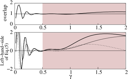
Figure 3: Top pannel: Total overlap $S$ of a trial function $\Phi_{\gamma}^{\theta}(x)=Cxe^{i\theta}e^{-\gamma x^{2}e^{2i\theta}}$ with the resonance eigenfuctions $\Psi_{k}^{\theta}$ of ${\hat{H}}_{\theta}$: $S=\left|\sum_{k=1}^{5}\langle\Psi_{k}^{*\theta}|\Phi_{\gamma}^{\theta}\rangle^{2}\right|$. The expansion is adequate in the shaded region. Deviations from $S=1$ for large $\gamma$ diminish when broader resonances are included in the expansion Ryaboy-NM . Bottom panel: left-hand-side of Eq.(6) (thick line), along with the contribution to it from the real part of the overlaps (solid) and the imaginary part (dotted).

Having established the plausibility of Eq.(7) for trial functions that can be expanded in terms of resonance wavefunctions, an analog of the Hohenberg-Kohn theorem follows. Two potentials $v_{\rm ext}^{[1]}$ and $v_{\rm ext}^{[2]}$ that do not support any bound state, and differ by more than a constant, cannot yield the same LER-density $n_{\theta}({\bf r})=\langle\Psi_{\scriptscriptstyle\rm LER}^{*\theta}|\hat{n}({\bf r}e^{i\theta})|\Psi_{\scriptscriptstyle\rm LER}^{\theta}\rangle$. To see this, assume that the two potentials could in fact give rise to the same LER-density:

$$\langle\Psi_{\scriptscriptstyle\rm LER}^{*[1]}|\hat{n}({\bf r}e^{i\theta})|\Psi_{\scriptscriptstyle\rm LER}^{[1]}\rangle=\langle\Psi_{\scriptscriptstyle\rm LER}^{*[2]}|\hat{n}({\bf r}e^{i\theta})|\Psi_{\scriptscriptstyle\rm LER}^{[2]}\rangle~{}~{},$$ (9)

where $\Psi_{\scriptscriptstyle\rm LER}^{[j]}$ is the LER-eigenstate of the Hamiltonian of Eq.(2) with external potential $v_{\rm ext}^{[j]}$. Using $\Psi_{\scriptscriptstyle\rm LER}^{[1]}$ as a trial function to estimate the lowest-energy eigenvalue of ${\hat{H}}_{\theta}^{[2]}$, we get by virtue of Eqs.(7) and (9) that ${\rm Re}\langle\Psi_{\scriptscriptstyle\rm LER}^{*[1]}|\hat{T}_{\theta}+\hat{V}_{ee,\theta}|\Psi_{\scriptscriptstyle\rm LER}^{[1]}\rangle>{\rm Re}\langle\Psi_{\scriptscriptstyle\rm LER}^{*[2]}|\hat{T}_{\theta}+\hat{V}_{ee,\theta}|\Psi_{\scriptscriptstyle\rm LER}^{[2]}\rangle$. But the opposite result is obtained by employing $\Psi_{\scriptscriptstyle\rm LER}^{[2]}$ as a trial function to estimate the lowest-energy eigenvalue of ${\hat{H}}_{\theta}^{[1]}$. We conclude that the original assumption of Eq.(9) is impossible if $v_{\rm ext}^{[1]}$ and $v_{\rm ext}^{[2]}$ differ by more than a constant.

To see the problem from a different perspective, we now examine the Levy-Lieb L79 ; L83 constrained search algorithm in the present context. The LER state is the one that, among all the normalized wavefunctions that make the complex energy $\langle\Psi_{\theta}^{*}|{\hat{H}}_{\theta}|\Psi_{\theta}\rangle$ stationary, minimizes the expectation value of ${\rm Re}\langle\Psi_{\theta}^{*}|{\hat{H}}_{\theta}|\Psi_{\theta}\rangle$. Following Levy, we perform the minimization in two steps, first constraining the search among all the wavefunctions yielding a prescribed complex density, $\{\Psi_{\theta}\mapsto n_{\theta}\}$, and then among all possible complex densities, $\{n_{\theta}\}$. The energy of the LER is then given by:

$${\cal E}_{\scriptscriptstyle\rm LER}=\mathop{\rm min}_{n_{\theta}}{\rm Re}\left[\int d{\bf z}~{}n_{\theta}({\bf z})v_{\rm ext}({\bf z})+{F_{\theta}[n_{\theta}]}\right]~{}~{}s.t.\left\{{\rm c1}\right\},$$ (10)

$${\rm Re}{F_{\theta}[n_{\theta}]}=\mathop{\rm min}_{\Psi_{\theta}\mapsto n_{\theta}}\left[{\rm Re}\langle\Psi_{\theta}^{*}|\hat{T}_{\theta}+\hat{V}_{ee,\theta}|\Psi_{\theta}\rangle\right]~{}~{}s.t.\left\{{\rm c2}\right\}$$ (11)

and constraints ${\rm c1}$ and ${\rm c2}$ are as discussed before:

$${\rm c1:} \int d{\bf z}n_{\theta}({\bf z})=N$$ (12)

$${\rm c2:} \frac{\delta}{\delta\Psi_{\theta}}{\langle\Psi^{*}_{\theta}|{\hat{H}}_{\theta}|\Psi_{\theta}\rangle}=0$$ (13)

In spite of the formal resemblance of Eq.(10) with the density-variational principle that serves as a starting point to derive Kohn-Sham equations, condition c2 makes of this a very different problem. It introduces a seemingly very complicated explicit dependence of $F_{\theta}[n_{\theta}]$ on $v_{\rm ext}$, preventing proof of the HKT analog.

But we now invoke Eq.(8). According to it, constraint c2 can be lifted altogether. The resulting (unconstrained) search of Eq.(11) defines a universal functional ${\rm Re}F_{\theta}[n_{\theta}]$, just as in the ground-state case. There is no explicit dependence of ${\rm Re}F_{\theta}[n_{\theta}]$ on $v_{\rm ext}$, and the HKT analog is established.

To access the lifetime of the LER, denote by $\bar{\Psi}_{\theta}$ the wavefunction that, within the set of functions yielding $n_{\theta}$, minimizes the real part of ${\langle\Psi_{\theta}^{*}|{\hat{H}}_{\theta}|\Psi_{\theta}\rangle}$ subject to the normalization constraint c1. It is a functional of $n_{\theta}$, $\bar{\Psi}_{\theta}[n_{\theta}]$. If we further define ${\rm Im}F_{\theta}[n_{\theta}]$ as the imaginary part of:

$${F_{\theta}[n_{\theta}]}={\langle\bar{\Psi}^{*}_{\theta}[n_{\theta}]|\hat{T}_{\theta}+\hat{V}_{ee,\theta}|\bar{\Psi}_{\theta}[n_{\theta}]\rangle}~{}~{},$$ (14)

then the inverse lifetime of the LER is given by the imaginary part of the sum of $F_{\theta}[n_{\theta}]$ and $\int d{\bf z}n_{\theta}({\bf z})v_{\rm ext}({\bf z})$.

When apart from being the resonance of lowest energy, the LER is also the resonance of longest lifetime, a typical case (e.g. our toy example), then Eq.(10) can be subsumed by a two-component minimization yielding at the same time the energy ${\cal E}$ and inverse lifetime $\Gamma=\hbar/\tau$ of the LER:

$$\left(\begin{array}[]{c}{\cal E}\\ \Gamma\end{array}\right)_{\scriptscriptstyle\rm LER}=\mathop{\rm min}_{n_{\theta}}\left(\begin{array}[]{c}{\rm Re}\\ -2{\rm Im}\end{array}\right)\left[\int{d{\bf z}~{}n_{\theta}({\bf z})v_{\rm ext}({\bf z})}+F_{\theta}[n_{\theta}]\right]$$ (19)

$$s.t.\{{\rm c1}\}$$

We have admittedly not addressed here the two fundamental questions that immediately arise: (1) What is the best way to cast the complex analog of the Kohn-Sham scheme for practical calculations? and (2) What is the functional form of $F_{\theta}[n_{\theta}]$? For one electron, it is simple to show that $F_{\theta}[n_{\theta}]=e^{-2i\theta}F[n_{\theta}]$, where $F[n_{\theta}]$ is the ground-state functional evaluated on the complex density.

Our derivation applies to the LER of unbound systems such as negatively charged atoms or molecules. However, using the Gel’fand-LevitanGELFAND equation it is quite straightforward to extend our formulation to systems that support also bound states. It has been shown already that using the Gel’fand Levitan equation one can remove bound states from the spectrum and obtain an effective potential which supports resonances onlyNM-Osvaldo . However, from a numerical point of view it might be a heavy task problem since the computation of new effective potentials that support the same resonances as the original problem, but not any of the $N$ bound states, requires the often prohibitive calculation of those bound-state wavefunctions. Our extension of the HKT for the LER of unbound systems holds also for atoms and molecules in the presence of external DC or AC electric fields, since the field-free ground (bound) state becomes a resonance state as the DC or AC fields are turned on (for the calculation of such resonances via complex scaling see refs. R82 and M98 ).

Negative electron affinities. We comment briefly on the computation of negative electron affinities as measured experimentally for many molecules via electron transmission spectroscopy JB87 . The standard definition of the electron affinity is: $A=E^{[N-1]}-E^{[N]}$ where $E^{[N-1]}$ is the ground-state energy of the neutral molecule, and $E^{[N]}$ is the ground-state energy of the negative ion. The latter is precisely equal to $E^{[N-1]}$ when the ion is not bound, so $A$ is zero in such cases. Confusion arises in practice when a finite basis set used in DFT calculations artificially binds the ion and predicts finite (negative) values for $A$. But the experiments measure a different quantity: $\tilde{A}=E^{[N-1]}-{\rm Re}E_{\scriptscriptstyle\rm LER}^{[N]}$ and this is not directly accessible via standard DFT calculations in the limit of an infnite basis-set. It is nonetheless interesting that $\tilde{A}-A$ is accurately given in many instances by the error associated with the use of a finite basis set (see discussion in ref.TP05 ).

Acknowledgements Useful discussions with Eric Heller are gratefully acknowledged.

References

- (1) W. Kohn, Rev. Mod. Phys. 71, 1253 (1999).
- (2) W. P. Reinhardt, Annu. Rev. Phys. Chem. 33, 223 (1982).
- (3) B.R. Junker, Adv. At. Mol. Phys. 18, 207 (1982).
- (4) N. Moiseyev, Phys. Rep. 302, 211 (1998).
- (5) P. Hohenberg and W. Kohn, Phys. Rev. 136, B 864 (1964).
- (6) O. Gunnarsson and B.I. Lundqvist, Phys. Rev. B 13, 4274 (1976)
- (7) U. von Barth, Phys. Rev. A 20, 1693 (1979).
- (8) R. Gaudoin and K. Burke, Phys. Rev. Lett. 93, 173001 (2004).
- (9) S.J. Buckman and C.W. Clark, Rev. Mod. Phys. 66, 539 (1994).
- (10) N. Moiseyev, Chem. Phys. Lett. 321, 469 (2000).
- (11) S.M. Valone, J.F. Capitani, Phys. Rev. A 23 2127 (1981).
- (12) M. Ernzerhof, J. Chem. Phys. 125, 124104 (2006).
- (13) I. Gilary, A. Fleischer and N. Moiseyev, Phys. Rev. A 72, 012117 (2005).
- (14) N. Moiseyev and L. S.Cederbaum, Phys. Rev A 72, 033605 (2005). Note that for spherically symmetric external potentials, and therefore the complex-scaled external potential operator in Eq.(2) is given by .
- (15) N. Moiseyev, P.R. Certain, and F. Weinhold Mol. Phys. 47, 585 (1982).
- (16) M. Levy, Proc. Nat. Acad. Sci. USA 76, 6062 (1979).
- (17) E.H. Lieb, Int. J. Quantum Chem. 24, 243 (1983).
- (18) E.R. Davidson, E. Engdahl, and N. Moiseyev, Phys. Rev. A 33, 2436 (1986).
- (19) V. Ryaboy and N. Moiseyev, J. Chem. Phys., 98, (1993).
- (20) I. M. Gel’fand and B. M. Levitan, Am Math. Soc. Trans. bf 1, 253 (1951).
- (21) N. Moiseyev and O. Goschinski, Chem. Phys. Lett., 120, 520 (1985).
- (22) K.D.Jordan and P.D.Burrow, Chem. Rev. 87, 557 (1987).
- (23) D.J. Tozer and F. De Proft, J. Phys. Chem. A 109, 8923 (2005).