Interplane and intraplane heat transport in quasi two-dimensional nodal superconductors

Abstract

We analyze the behavior of the thermal conductivity in quasi-two dimensional superconductors with line nodes. Motivated by measurements of the anisotropy between the interplane and intraplane thermal transport in CeIrIn₅ we show that a simple model of the open Fermi surface with vertical line nodes is insufficient to describe the data. We propose two possible extensions of the model taking into account a) additional modulation of the gap along the axial direction of the open Fermi surface; and b) dependence of the interplane tunneling on the direction of the in-plane momentum. We discuss the temperature dependence of the thermal conductivity anisotropy and its low $T$ limit in these two models and compare the results with a model with a horizontal line of nodes (“hybrid gap”). We discuss possible relevance of each model for the symmetry of the order parameter in CeIrIn₅, and suggest further experiments aimed at clarifying the shape of the superconducting gap.

I Introduction

Symmetry classification of possible gap structures established the framework for separating conventional superconductors from their unconventional counterparts Blount (1985); Volovik and Gor’kov (1985); Sigrist and Ueda (1991). Superconductors with the order parameters that transform according to the trivial irreducible representation of the point symmetry group of the crystal are usually labeled conventional. If the order parameter transforms according to a non-trivial representation of the same group, the superconductor is called unconventional.

In the latter class the symmetry of the order parameter is lower than the full group symmetry. This lowering of symmetry is usually believed to be related to strong repulsive Coulomb interactions and specific pairing mechanisms (for example, due to magnetic fluctuations). As a result, determining the gap structure is one of the crucial steps in testing our understanding of the origin of superconductivity in a given material. An important group of unconventional superconductors are those with order parameter that vanishes (has nodes) for some directions at the Fermi surface.

Thermal conductivity is an exceptionally powerful probe for testing the shape of the gap in nodal superconductors since only the unpaired electrons (with momenta close to the nodal directions) carry entropy. The presence or absence of the nodes, and sometimes their type (point or line), can be inferred from the dependence of the thermal conductivity on the magnetic field and temperature. An additional test for the existence of line nodes is the so-called universality of the low-temperature coefficient of the thermal conductivity, $a_{0}=\lim_{T\rightarrow 0}\kappa/T$  Lee (1993); Sun and Maki (1995); Graf et al. (1996). The universal behavior refers to the relative insensitivity of $a_{0}$ to the concentration of the impurity atoms and to the details of the scattering on individual impurity centers Durst and Lee (2000). Physically, since impurity scattering is pairbreaking, it generates near-nodal quasiparticles which can carry heat, and whose lifetime is, in turn, is limited by scattering on the same impurities. For linear nodes the two effects cancel nearly exactly. In the high-T_c cuprates, for example, the quantitative agreement between theoretical estimates of $a_{0}$ and the measured thermal conductivity was established Taillefer et al. (1997); Chiao et al. (2000). However, determining the location of the nodes in the momentum space from such measurements is much harder.

The most direct tests measure the variation in the heat transport with the orientation of the applied magnetic field with respect to the nodal directions Yu et al. (1995); Aubin et al. (1997); Izawa et al. (2003, 2002a); Watanabe et al. (2004); Izawa et al. (2001, 2002b). Long before such experiments were attempted, it was proposed that the anisotropy of the thermal conductivity along two different directions as a function of temperature allows to infer information about the gap structure Arfi et al. (1989); Fledderjohann and Hirschfeld (1995). Essentially, the measurement determines the predominant direction of the Fermi velocity for the nodal quasiparticles. Combined with the knowledge of the Fermi surface, measurements of the evolution of the anisotropy in the superconducting state impose stringent constraints on the possible loci of the nodes.

This method was applied to UPt₃Lussier et al. (1994), and the results argued convincingly for a line of nodes at $k_{z}=0$. The main reason this experiment did not uniquely determined the gap structure is that theoretically expected results depend on the detailed shape of the Fermi surface and the superconducting gap, i.e. on the basis functions for the particular representation Norman and Hirschfeld (1996). This detail apart, it is believed that the measurement provides a good test for the horizontal vs. vertical linear nodes.

Very recently the anisotropy of the thermal conductivity along inequivalent crystalline directions was measured in heavy fermion CeIrIn₅ by Shakeripour et al. Shakeripour et al. (2006). The ratio of the $c$-axis to the in-plane thermal conductivity, $\kappa_{c}/\kappa_{a}$, rapidly decreases in the superconducting state. Similarity of the anisotropy evolution to that for UPt₃, where equatorial line of nodes is believed to exist, led the authors of Ref. Shakeripour et al., 2006 to suggest that the superconducting gap in CeIrIn₅ also has a horizontal line of nodes. This is surprising since CeCoIn₅, a close relative of CeIrIn₅, has vertical lines of nodes Izawa et al. (2001); Aoki et al. (2004), and the prevailing belief is that the two compounds are quite similar (although some evidence points to different origin of superconductivity in the two systems Nicklas et al. (2004)).

Consequently, in this paper we re-visit the analysis of the temperature dependence and the anisotropy of the thermal conductivity in nodal superconductors. Since both de Haas - van Alphen measurements, and band structure calculations show that CeIrIn₅ has an open, quasi-two dimensional piece of the Fermi surface with significant $f$-electron contribution Haga et al. (2001), our main focus here is on such anisotropic systems. We discuss the implications of the measurements for the symmetry of the order parameter, and compare the anisotropy of the thermal conductivity for several models relevant not only to CeIrIn₅, but also to other systems with a quasi-two dimensional Fermi surface.

The remainder of the paper is organized as follows. In next section we introduce the basic experimental facts and theoretical considerations, formulating the models. The subsequent sections are devoted to the analysis of the proposed models. We then critically compare our results with experiment, and propose further measurements to test the gap symmetry in CeIrIn₅.

II Experimental background

CeIrIn₅ is a member of the so called 115 series, which also include CeCoIn₅ and CeRhIn₅. While in the Rh system the $f$-electrons of Ce remain localized and undergo antiferromagnetic ordering, both Ir and Co compounds are paramagnetic heavy fermion metals. In both systems de Haas-van Alphen measurements and the band structure calculations indicate that a major sheet of the Fermi surface is quasi-two dimensional, although the energy dispersion along the $c$-axis is substantial, as evidenced by a very moderate anisotropy ($\sim 2$) between the out of plane and in-plane normal state transport coefficients. In contrast to CeCoIn₅, which is a highly unconventional metal, likely close to a quantum critical point at finite magnetic field Bianchi et al. (2003); Paglione et al. (2003), CeIrIn₅ near the superconducting phase is a good Fermi liquid, and therefore its excitations should be adequately described by the calculations in the Fermi-liquid framework.

Both CeIrIn₅ and CeCoIn₅ are ambient pressure superconductors, and Knight shift measurements indicate singlet pairing Kohori et al. (2001); Zheng et al. (2001). Specific heat and in-plane thermal conductivity measurements Movshovich et al. (2001), as well as penetration depth Chia et al. (2003) and spin-lattice relaxation rate Kohori et al. (2001); Zheng et al. (2001), show the existence of line nodes. In CeCoIn₅ there is overwhelming evidence for the vertical line nodes from the anisotropy of the thermal conductivity and specific heat under rotated magnetic field Izawa et al. (2001); Aoki et al. (2004), and from the tunneling into the Andreev bound states Park et al. (2005). Given the strong similarities between the Fermi surfaces it is tempting to conclude that the gap structure is similar in the two materials. There is, however, evidence pointing towards differences in the origin (and hence possibly in the type) of the superconducting state of the Co and Ir compounds Nicklas et al. (2004).

Authors of Ref.Shakeripour et al., 2006 measured the temperature dependence of the thermal conductivity in CeIrIn₅ along two inequivalent crystalline directions, $\kappa_{c}(T)$ (out of plane) and $\kappa_{a}(T)$ (in plane), and made two significant observations: a) The ratio $R(T)=\kappa_{c}/\kappa_{a}$ is nearly temperature-independent above the superconducting transition temperature, $T_{c}$, but is rapidly reduced with $T$ at $T<0.5T_{c}$ (Note that inelastic scattering yields a peak in thermal conductivity just below $T_{c}\sim 0.4$ K, which may lead to the decrease of $R(T)$ appearing very pronounced); b) The low $T$ limit of the in-plane $\kappa_{a}/T$ appears universal, but the interplane $\kappa_{c}/T$ does not show the universal limit. Our goal below is to examine the possible origin and implications of this result.

III Basic considerations and models

Independently of the choice of theoretical model, the results a) and b) above imply, prima facie, that the effect of superconductivity on the quasiparticles with the Fermi velocity predominantly in the plane is different from that for the quasiparticles moving along the c-axis: the states that carry entropy along the $c$-axis have a larger “effective gap” than those carrying heat current in the plane. Several processes of different physical origin may lead to this behavior. In the following we do not consider inelastic scattering; this is appropriate at low temperatures, $T\ll T_{c}$. The range of temperatures in Ref. Shakeripour et al., 2006 where the inelastic scattering can be neglected is not immediately clear from the data, note, however, that, if the inelastic scattering is isotropic, our conclusions regarding the anisotropy of the thermal transport are not affected.

Since the Fermi surface of CeIrIn₅ has several sheets, it is, of course, possible that the multiband effects are responsible for the observed behavior. However, without a microscopic theory detailing the gaps on each of the sheets, reaching reliable conclusions about the agreement between theory and experiment seems impossible, while phenomenological multiband theory has too many fitting parameters to seriously constrain possible gap structures. We aim to construct a minimal model that captures the essential physics of the the experimental observations, and therefore restrict ourselves to considering one electronic band.

Since most band structure and dHvA analyses suggest an important role of the quasi-two dimensional (open along the $c$-axis) band, we choose such a band for our approach. We approximate it by a simple nearest neighbor tight binding expression

$$\epsilon(\bm{k})=\frac{k_{x}^{2}+k_{y}^{2}}{2m}-2t(\bm{k})\cos(k_{z}c),$$ (1)

where $k_{i}$ are the components of the quasiparticle momentum, ${\bm{k}}$, $c$ is the lattice spacing in the $z$ direction, $m$ is the effective mass, and $t(\bm{k})$ is the interplane tunneling matrix element. In all but one of our models we take $t(\bm{k})$ to be momentum-independent. We show below however, that the model with $\bm{k}$-dependent interplane tunneling that provides a viable path towards explaining the experimental results, even with the assumption of vertical, rather than horizontal, nodes.

We consider singlet order parameters, and begin with the simple model of vertical line nodes similar to the order parameter in CeCoIn₅, introducing the azimuthal in-plane angle $\phi=\arctan k_{y}/k_{x}$,

• Model A: $t(\bm{k})=t$, and
                 $\Delta(\bm{k})=\Delta_{0}\cos 2\phi$.

We show in the next section that this model is incompatible with the experimental observations. Physically, the Fermi surface is cylindrically symmetric and the gap depends only on the azimuthal angle, $\phi$, while the $z$-axis component of the Fermi velocity is $\phi$-independent. As we show below in Sec. V, these conditions ensure that the ratio $\kappa_{c}/\kappa_{a}\equiv\kappa_{zz}/\kappa_{xx}$, is temperature-independent even in the superconducting state.

This constraint needs to be relaxed to explain the experimental results, and we consider several possible models. First, we show that for a tight-binding Fermi surface it can be expected, from microscopic considerations, that the gap also acquires a weak modulation along the $c$-direction, while retaining vertical lines of nodes, and therefore consider

• Model B: $t(\bm{k})=t$, and
                 $\Delta(\bm{k})=\Delta_{0}(1+\delta\cos k_{z}c)\cos 2\phi$.

While in this model there exists a temperature-dependent anisotropy, we find that this dependence is generally weak, and hence unlikely to provide a satisfactory explanation of the experimental observations (although we cannot exclude it).

In the second approach to lifting the constraints of model A we consider a situation with vertical line nodes, but where the nodal quasiparticles are less efficient than the normal electrons (on average) in transporting heat along the $c$-axis compared to the $xy$ plane. To model this we note that the measured and calculated Fermi surface of CeIrIn₅ is not rotationally symmetric Haga et al. (2001), and that the energy dispersion of the electrons along the $z$-axis clearly depends on the direction of the in-plane momentum. This dependence is expected in the $D_{4h}$ symmetry, and $t(\bm{k})$ is determined by the structure of the overlapping wave functions for the quasi-two dimensional band. We therefore introduce the angle dependence into the interplane tunneling, preserving the crystal symmetry in the plane, and propose

• Model C: $t(\bm{k})=t_{0}+t_{1}\cos^{2}2\phi$, and
                $\Delta(\bm{k})=\Delta_{0}\cos 2\phi$.

For $t_{1}>0$ the interplane tunneling is smaller for the nodal quasiparticles than for antinodal ones, which ensures the $T$-dependence of the anisotropy ratio. The situation is somewhat reminiscent of that in the high-T_c cuprates where, in the absence of orthorhombic distortion, the interplane tunneling of the nodal quasiparticles is suppressed, i.e. $t_{0}=0\$ Xiang and Wheatley (1996), and therefore the observed temperature dependence of the Josephson plasma resonance frequency Gaifullin et al. (1999) and the $c$-axis penetration depth Panagopoulos et al. (1997); Hosseini et al. (1998) is different from that suggested by the simple density of states power counting. We show that such a model gives a significant temperature-dependent anisotropy of the thermal conductivity.

Finally, we consider a model with horizontal, rather than vertical line nodes, similar to the hybrid $E_{1g}$ gap proposed for UPt₃, with broken time-reversal symmetry. The basis function of the representation is described as $k_{z}(k_{x}+ik_{y})$. For open Fermi surface we require periodicity along the $z$-direction, and the appropriate basis function is $(k_{x}+ik_{y})\sin k_{z}c$. The excitation spectrum and the thermal conductivity are only sensitive to the gap amplitude, $|\Delta(\bm{k})|=k_{\perp}|\sin k_{z}c|$, where $k_{\perp}=(k_{x}^{2}+k_{y}^{2})^{1/2}$. Since our consideration of Model B shows (see the analysis below) that weak modulation does not change the anisotropy qualitatively, we ignore it, and consider

• Model D: $t(\bm{k})=t$, and
                $|\Delta(\bm{k})|=\Delta_{0}|\sin k_{z}c|$.

We show that, this model also gives a substantially temperature-dependent ratio $\kappa_{zz}/\kappa_{xx}$. Moreover, we point out that from the data of Ref. Shakeripour et al., 2006 it is impossible to distinguish Model C from Model D, and suggest further measurements to probe the gap structure in CeIrIn₅.

We are now ready to consider each model in detail. In order to make connection with experiment, we largely focus on the thermal conductivity and its anisotropy

$$R(T)=\frac{\kappa_{zz}(T)}{\kappa_{xx}(T)}.$$ (2)

We begin by briefly looking at the normal state properties.

IV Normal State

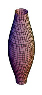
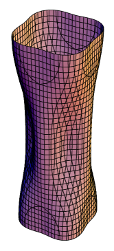
Figure 1: Fermi surfaces for models considered in the paper. Left panel: Models A,B, and D. Right panel: Model C. Notice the similarity between the Fermi surface shown in that panel and the Fermi surface suggested for CeIrIn₅ in Ref. Haga et al., 2001.

The Fermi surfaces for the models A through D are shown in Fig. 1. In each case we transform to the cylindrical coordinates and parameterize the Fermi surface by the azimuthal angle $\phi=\arctan k_{y}/k_{x}$, and the c-axis quasimomentum $k_{z}$. The Jacobian of the transformation from variables $k_{x},k_{y},k_{z}$ to variables $\epsilon,k_{z},\phi$ is unity, and therefore no angle-dependence of the normal state density of states appears. We denote the Fermi energy $E_{F}$, and define the Fermi momentum at $k_{z}=\pm\pi/2c$ as $k_{F}=\sqrt{2mE_{F}}$.

In models A, B, D above the tunneling $t$ is $\phi$-independent. In that case, the radius of the Fermi surface is $k_{0}(k_{z})=k_{F}\sqrt{1+(2t/E_{F})\cos(k_{z}c)}$, and the components of the Fermi velocity are

$$v_{x} = \frac{k_{0}\cos\phi}{m}=v_{F}\sqrt{1+(2t/E_{F})\cos(k_{z}c)}\cos\phi,$$ (3a)

$$v_{y} = \frac{k_{0}\cos\phi}{m}=v_{F}\sqrt{1+(2t/E_{F})\cos(k_{z}c)}\sin\phi,$$ (3b)

$$v_{z} = 2tc\sin(k_{z}c)=\frac{t}{E_{F}}(k_{F}c)v_{F}\sin(k_{z}c),$$ (3c)

where $v_{F}=k_{F}/m$. In the normal state the anisotropy of the transport coefficients is given simply by

$$R_{n}\equiv\frac{\sigma_{zz}}{\sigma_{xx}}=\frac{\kappa_{zz}/T}{\kappa_{xx}/T}=\frac{\langle v_{z}^{2}\rangle}{\langle v_{x}^{2}\rangle},$$ (4)

where the average over the Fermi surface is

$$\langle A\rangle=\int_{0}^{2\pi}\frac{d\phi}{2\pi}\int_{-\pi}^{\pi}\frac{d\chi_{z}}{2\pi}\,A(\phi,k_{z}),\mbox{ and }\chi_{z}=k_{z}c.$$ (5)

For the simple model above $R_{n}=(t/E_{F})^{2}(k_{F}c)^{2}$.

We can obtain a very rough estimate of the parameter values relevant for CeIrIn₅ from the dHvA measurements and the band structure calculations Haga et al. (2001). For the quasi-cylindrical piece of the Fermi surface the typical radius is 1/5 of the Brillouin Zone size, $k_{F}\approx 2\pi/(5a)$, where $a$ is the in-plane lattice constant. In this material $c/a\sim 1.6$, so that $k_{F}c\approx 2$. The normal state resistivity ratio, $R_{n}\sim 0.4$, implying $t/E_{F}\sim 0.3$.

For model C the situation is slightly more complex. We still have

$$v_{z}=2t(\phi)c\sin(k_{z}c)=2t(\phi)c\sin\chi_{z},$$ (6)

and therefore

$$\langle v_{z}^{2}\rangle=\frac{v_{F}^{2}}{2}(k_{F}c)^{2}\left[\frac{t_{0}^{2}}{E_{F}^{2}}+\frac{t_{0}t_{1}}{E_{F}^{2}}+\frac{3}{8}\frac{t_{1}^{2}}{E_{F}^{2}}\right].$$ (7)

At arbitrary in-plane $k$ the $x$-component of the velocity is

$$v_{x}=\frac{k\cos\phi}{m}+\frac{2t_{1}}{k}\sin\phi\sin 4\phi\cos\chi_{z},$$ (8)

and, consequently, at the Fermi surface,

$$\langle v_{x}^{2}\rangle=\frac{v_{F}^{2}}{2}+v_{F}^{2}\frac{t_{1}^{2}}{E_{F}^{2}}\left<\frac{\sin^{2}\phi\sin^{2}4\phi\cos^{2}\chi_{z}}{1+2t(\phi)/E_{F}\cos\chi_{z}}\right>.$$ (9)

Since we work in the regime $t_{0,1}/E_{F}\ll 1$, we can ignore the corrections from the term $t(\phi)/E_{F}$ in the denominator as they appear only at the order $(t/E_{F})^{4}$, and write

$$\langle v_{x}^{2}\rangle=\frac{v_{F}^{2}}{2}\left[1+\frac{3}{16}\frac{t_{1}^{2}}{E_{F}^{2}}\right].$$ (10)

For the conductivity anisotropy of 2.5 cited above, the maximal value of $t_{1}/E_{F}$, when there is no $t_{0}$ component, is approximately $(t_{1}/E_{F})^{2}\approx 4/15$, which corresponds to the contribution of the second term of less than 5% to the in-plane transport in the normal state. Its effect in the superconducting state is even smaller, since the $t_{1}$-dependent part of $v_{x}$ vanishes along the nodal directions. Consequently, we ignore the $t_{1}$-dependent contribution to the in-plane transport hereafter.

V Model A: constant hopping, vertical line nodes

The thermal conductivity of a superconductor with the gap function whose average over the Fermi surface vanishes is given by Norman and Hirschfeld (1996); Kübert and Hirschfeld (1998)

$$\frac{\kappa_{ii}}{T}=\frac{N_{0}}{4}\int_{0}^{\infty}\frac{d\omega}{T}\left(\frac{\omega}{T}\right)^{2}{\rm sech}^{2}\left(\frac{\omega}{2T}\right)K_{i}(\omega,T),$$ (11)

$$K_{i}(\omega,T)=\frac{1}{\widetilde{\omega}_{1}\widetilde{\omega}_{2}}\>{\rm Re}\left<v_{i}^{2}\>\frac{\widetilde{\omega}^{2}+|\widetilde{\omega}|^{2}-2|\Delta_{\bf k}|^{2}}{\sqrt{\widetilde{\omega}^{2}-|\Delta_{\bf k}|^{2}}}\right>\;.$$

Here $N_{0}$ is the normal state density of states, and the renormalized frequency $\widetilde{\omega}=\widetilde{\omega}_{1}+i\widetilde{\omega}_{2}=\omega-\Sigma(\widetilde{\omega})$, where $\Sigma$ is the self-energy due to impurity scattering. For the model with $\Delta_{\bf k}=\Delta_{0}\cos 2\phi$, and the hopping that is $\phi$-independent, we immediately find for different orientations of the heat current

$$\left<v_{i}^{2}\>\frac{\widetilde{\omega}^{2}+|\widetilde{\omega}|^{2}-2|\Delta_{\bf k}|^{2}}{\sqrt{\widetilde{\omega}^{2}-|\Delta_{\bf k}|^{2}}}\right>=\frac{2\eta_{i}}{\pi}$$ (12)

$$\qquad\qquad\times\left[\widetilde{\omega}\>{\rm E}\left(\frac{\Delta_{0}}{\widetilde{\omega}}\right)+\frac{|\widetilde{\omega}|^{2}-\widetilde{\omega}^{2}}{2\widetilde{\omega}}\>{\rm K}\left(\frac{\Delta_{0}}{\widetilde{\omega}}\right)\right]\;,$$

where $E$ and $K$ are the complete elliptic integrals, and

$$\eta_{x}=v_{F}^{2},\qquad\eta_{z}=(2tc)^{2}.$$ (13)

Therefore the anisotropy of the thermal conductivity in the superconducting state remains unchanged compared to the normal state, $R_{s}=R_{n}=(t/E_{F})^{2}(k_{F}c)^{2}$. Moreover, in this model the universal (nearly independent on impurity concentration) low temperature limit, obtained from Eq.(12), is Lee (1993); Sun and Maki (1995); Graf et al. (1996); Norman and Hirschfeld (1996)

$$a_{0,i}=\lim_{T\rightarrow 0}\frac{\kappa_{i}}{T}=\frac{\pi}{6}\frac{N_{0}\eta_{i}}{\sqrt{\gamma^{2}+\Delta_{0}^{2}}}E\left(\frac{\Delta_{0}}{\sqrt{\gamma^{2}+\Delta_{0}^{2}}}\right),$$ (14)

for both in-plane and out of plane directions. In Eq.(14) $\gamma$ is the low-energy scattering rate, $\widetilde{\omega}(\omega=0)=i\gamma$, and $E$ is the complete elliptic integral. For clean superconductors, $\gamma\ll\Delta_{0}$, and we have

$$\frac{1}{\sqrt{\gamma^{2}+\Delta_{0}^{2}}}E\left(\frac{\Delta_{0}}{\sqrt{\gamma^{2}+\Delta_{0}^{2}}}\right)\approx\frac{1}{\Delta_{0}}+O\left(\frac{\gamma^{2}}{\Delta_{0}^{2}}\right),$$ (15)

so that $a_{0,i}=\eta_{i}\pi N_{0}/(6\Delta_{0})$, universal and independent of the impurity scattering rate.

This constant and temperature independent ratio $R_{s}(T)$ is in contradiction to the experimental measurements of Ref. Shakeripour et al., 2006, and therefore model A does not provide a satisfactory description of the superconducting state of CeIrIn₅.

VI Model B: modulated gap

VI.1 Microscopic justification

The symmetry classification does not uniquely determine the functional form of the superconducting gap around the Fermi surface. The gap can be given by any combination of the basis functions transforming according to the chosen irreducible representation. For example, in a cubic system, both a constant gap and that varying as $k_{x}^{4}+k_{y}^{4}+k_{z}^{4}$ have the same symmetry properties.

Of course, any $\bm{k}$-space variation of the gap beyond that imposed by symmetry requirements costs condensation energy, and therefore, all other things being equal, the simplest basis functions often provide the most stable superconducting state. A conventional superconductor with a spherical Fermi surface strongly prefers a fully isotropic gap, while a strongly anisotropic quasi two-dimensional system with a circular Fermi surface and the dominant pairing in the $B_{1g}$ channel is likely to have the gap with the $k_{x}^{2}-k_{y}^{2}$ momentum dependence. This is the reason for using the familiar notation of $s$-wave for the former case, and $d_{x^{2}-y^{2}}$ for the latter.

On the other hand, superconductivity is an instability of the Fermi surface towards pairing, and therefore it is natural to expect that in real materials with complex Fermi surfaces the gap structure is also more complex. The correct gap can only be determined from the microscopic theory of superconductivity. To solve Eliashberg equations in superconductors with electron-phonon mediated pairing, Allen introduced the Fermi surface harmonics Allen (1976), which have the symmetry of the Fermi surface, are orthonormal, and are convenient basis functions for the expansion of the superconducting pairing field.

In the absence of microscopic theory we use similar symmetry arguments, and go beyond lowest order basis functions. For simplicity, we continue to consider the $d_{x^{2}-y^{2}}$ gap symmetry, $\Delta(\bm{\hat{k}})\propto\cos 2\phi$; all our considerations apply equally well to other gaps with vertical line nodes, such as $d_{xy}$. Choice of this symmetry determines the irreducible representation of the crystal point group. In a system with the Fermi surface open along the c-axis, we need to add to this point group the invariance with respect to translations by a reciprocal lattice vector along $z$. In the even (odd) channel the basis functions for translation are $\cos nk_{z}c$ ($\sin nk_{z}c$), with $n$ integer. Therefore quite generally the singlet $d_{x^{2}-y^{2}}$ gap has the form

$$\Delta(\bm{\hat{k}})=\sum_{n}\Delta_{n}\cos(nk_{z}c)\cos 2\phi.$$ (16)

Similar interaction for $s$-wave pairing was considered by Bulaevskii and Zyskin Bulaevskii and Zyskin (1990), and for $d$-wave symmetry by Rajagopal and Jha Rajagopal and Jha (1996); Jha and Rajagopal (1997). Note that since even powers of $k_{z}$, and therefore $\cos(nk_{z}c)$, transform according to a trivial representation of the tetragonal point group, the functions with different $n$ belong to the same representation and can be mixed.

The degree of mixing is, of course, determined by the pairing interaction. We consider a separable model,

$$V(\bm{\hat{k}},\bm{\hat{k}^{\prime}})=\Phi(\bm{\hat{k}})\Phi(\bm{\hat{k}^{\prime}}),$$ (17)

where

$$\Phi(\bm{\hat{k}})=\sum_{n}V_{n}\cos(nk_{z}c)\cos 2\phi.$$ (18)

To illustrate the behavior of the model, and to be consistent with keeping only the nearest neighbor layer hopping in the energy dispersion, Eq.(1), we truncate the expansion at $n=1$, so that

$$V(\bm{\hat{k}},\bm{\hat{k}^{\prime}})=V_{0}\left[1+\lambda_{1}(\cos\chi_{z}+\cos\chi_{z}^{\prime})+\lambda_{2}\cos\chi_{z}\cos\chi_{z}^{\prime}\right]\cos 2\phi\cos 2\phi^{\prime}.$$ (19)

To the same accuracy the gap is given by

$$\Delta(\bm{k})=\Delta_{0}\left[1+\delta\cos\chi_{z}\right]\cos 2\phi,$$ (20)

and is determined from the self-consistency equation (for pure superconductor in the weak-coupling limit)

$$\Delta(\bm{k})=\pi T\sum_{|\omega_{n}|<\Omega_{0}}\int_{-\pi}^{\pi}\frac{d\chi_{z}}{2\pi}\int_{0}^{2\pi}\frac{d\phi}{2\pi}\frac{\widetilde{V}(\bm{\hat{k}},\bm{\hat{k}^{\prime}})\Delta(\bm{\hat{k}^{\prime}})}{\sqrt{\omega_{n}^{2}+\Delta^{2}(\bm{\hat{k}^{\prime}})}}.$$ (21)

Here $\widetilde{V}(\bm{\hat{k}},\bm{\hat{k}^{\prime}})=N_{0}V(\bm{\hat{k}},\bm{\hat{k}^{\prime}})$, $\omega_{n}=\pi T(2n+1)$ are the fermionic Matsubara frequencies, and $\Omega_{0}$ is the cutoff energy for the pairing interaction.

Formally, the gap given by Eq.(20) allows for a horizontal line of nodes when $\delta>1$. This is, however, physically unlikely. In the interaction $V(\bm{\hat{k}},\bm{\hat{k}^{\prime}})$ above, $\lambda_{2}$ is the relative strength of the pairing in neighboring planes compared to the in-plane pairing, so that $|\lambda_{2}|<1$. Generally we also expect $\lambda_{1}\sim t/E_{F}<1$  Bulaevskii and Zyskin (1990), so that the gap modulation along the $c$-axis is insufficient to produce horizontal lines of nodes. Inversely, if the interaction strengths in different channels in Eq.(19) are comparable, we cannot truncate the expansion at the lowest order terms. Therefore, while in principle the symmetry considerations allow the gap in Eq.(20) to have both horizontal and vertical nodes, the model considered here can only be used if it yields small to moderate values of $\delta$.

Consider first the linearized equations for the transition temperature, $T_{c}$. Introducing dimensionless coupling constant $g=N_{0}V_{0}$, we find that $T_{c}$ and $\delta$ satisfy

$$1 = \frac{g}{2}\left[1+\frac{\lambda_{1}\delta}{2}\right]\ln\frac{2\gamma_{E}\Omega_{0}}{\pi T_{c}},$$ (22a)

$$\delta = \frac{g}{2}\left[\lambda_{1}+\frac{\lambda_{2}\delta}{2}\right]\ln\frac{2\gamma_{E}\Omega_{0}}{\pi T_{c}}.$$ (22b)

Here $\gamma_{E}\approx 0.58$ is the Euler’s constant. Note that in the absence of the $\lambda_{1}$ term in the pairing interaction the equations for the temperatures of the transition into the states $\Delta_{0}\cos 2\phi$ and $\Delta_{1}\cos\chi_{z}\cos 2\phi$ decouple, and each is reduced to the standard BCS expression, $T_{c}^{(n)}=(2\gamma_{E}/\pi)\Omega_{0}\exp(-2/g_{eff}^{(n)})$, with the effective coupling constants in the $\cos n\chi_{z}$ channels $g$ and $\lambda_{2}g/2$ for $n=0$ and $n=1$ respectively. For $\lambda_{2}/2<1$ this implies that $T_{c}^{(0)}>T_{c}^{(1)}$, so that the simple $\cos 2\phi$ gives the dominant order parameter.

For the generic case $\lambda_{1}\neq 0$, however, the two channels are coupled, and the transition occurs directly into the c-axis modulated state $\Delta=\Delta_{0}(1+\delta\cos\chi_{z})\cos 2\phi$. The transition temperature is

$$T_{c}=\frac{2\gamma_{E}}{\pi}\Omega_{0}\exp(-2x_{0}/g),$$ (23)

where

$$x_{0} = \frac{2}{1+\lambda_{2}/2+D^{1/2}},$$ (24)

$$D = \left(1-\lambda_{2}/2\right)^{2}+2\lambda_{1}^{2}.$$ (25)

We assumed that the coupling $\lambda_{2}$ is not too repulsive. The transition temperature depends on the magnitude, but not on the sign of $\lambda_{1}$. On the other hand, the modulation, $\delta=2(x_{0}^{-1}-1)/\lambda_{1}$, depends on the sign of $\lambda_{1}$, and can be either positive or negative.

The modulation amplitude, $\delta$, is generally $T$-dependent. Consider the self-consistency equation at $T<T_{c}$,

$$1=g\pi T\sum_{|\omega_{n}|<\Omega_{0}}\int_{-\pi}^{\pi}\frac{d\chi_{z}^{\prime}}{2\pi}\int_{0}^{2\pi}\frac{d\phi^{\prime}}{2\pi}\left[1+\lambda_{1}\cos\chi_{z}^{\prime}\right]\frac{\left[1+\delta\cos\chi_{z}^{\prime}\right]\cos^{2}2\phi^{\prime}}{\sqrt{\omega_{n}^{2}+\Delta_{0}^{2}(1+\delta\cos\chi_{z}^{\prime})^{2}\cos^{2}2\phi^{\prime}}}$$ (26a)

$$\delta=g\pi T\sum_{|\omega_{n}|<\Omega_{0}}\int_{-\pi}^{\pi}\frac{d\chi_{z}^{\prime}}{2\pi}\int_{0}^{2\pi}\frac{d\phi^{\prime}}{2\pi}\left[\lambda_{1}+\lambda_{2}\cos\chi_{z}^{\prime}\right]\frac{\left[1+\delta\cos\chi_{z}^{\prime}\right]\cos^{2}2\phi^{\prime}}{\sqrt{\omega_{n}^{2}+\Delta_{0}^{2}(1+\delta\cos\chi_{z}^{\prime})^{2}\cos^{2}2\phi^{\prime}}}$$ (26b)

In the linearized form considered above, all the terms in the integrand linear in $\cos\chi_{z}^{\prime}$, vanish by symmetry. On the other hand, below $T_{c}$, when $\Delta^{2}$ term in the denominator is important, these terms give a finite contribution to the gap equation. Moreover, in contrast to the conventional “one-channel” systems, the cutoff frequency $\Omega_{0}$ cannot be removed from the self-consistency equations completely. As a consequence, $\delta$ acquires temperature dependence.

Of course, in the weak coupling limit this dependence is insignificant: in both integrals in Eq.(26) the greatest contribution is from the range $\Delta_{0}\ll\omega_{n}\leq\Omega_{0}$, and therefore essentially insensitive to the absence or presence of the gap. In most situations the dependence on the cutoff vanishes already for $\Omega_{0}/T_{c}\geq 10$. This is seen from the self-consistently determined temperature evolution of the gaps in the two channels computed using Eqs.(26) and shown in the left panel of Fig.2. The corresponding plot of the modulation, $\delta$, in the right panel of Fig.2 demonstrates that the modulation is temperature-independent for most parameter values.

We find that one exception is the somewhat artificial situation when a) the bare transition temperatures into the two states are very close, $\lambda_{2}\approx 2$ so that $T_{c}^{(0)}\approx T_{c}^{(1)}$, and b) $\lambda_{1}\ll 1$. While $\delta$ is still temperature-independent for $\Omega_{0}/T_{c}\rightarrow\infty$, the temperature variations persist to large values of the cutoff, see Fig.2. Part of the reason is that the value of $\delta(\lambda_{1}\rightarrow 0,\lambda_{2}\rightarrow 2)$ at $T_{c}$ obtained above depends on the order in which the limits are taken: setting $\lambda_{2}=2$ first gives $\delta=\sqrt{2}$, while taking the limit $\lambda_{1}\rightarrow 0$ first for a finite value of $1-\lambda_{2}/2$ yields $\delta=0$.

Physically, at the point $\lambda_{2}=2,\lambda_{1}=0$ the linearized equations, Eq.(22), decouple, and give no information on the values of $\Delta_{0}$ and $\Delta_{1}=\Delta_{0}\delta$. As is well known, the gap amplitudes are determined by the fourth order terms in the Ginzburg-Landau expansion of the free energy, or, equivalently, by the third order terms in the gap equations. We find that inclusion of such terms gives three different possible solutions for $\Delta_{0}$ and $\Delta_{1}$. Two of them are trivial, $\Delta_{0}\neq 0,\Delta_{1}=0$ (lowest energy, as expected), and $\Delta_{0}=0,\Delta_{1}\neq 0$. However, we find that there is a third solution with $\Delta_{1}/\Delta_{0}=\delta=const$, which has the highest energy of the three. At the same time for $\lambda_{2}=2$ and any finite $\lambda_{1}$ $\delta=const$ corresponds to the lowest free energy, which suggests a singular limit $\lambda_{1}\rightarrow 0$. This is confirmed by carrying our the expansion of $\delta$ in $1-T/T_{c}$, at finite $\lambda_{1}$, where we find that the coefficients are singular for $\lambda_{2}=2$. This suggests a strong dependence of the energies of the three stationary points on parameters, and on temperature.

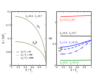
Figure 2: Temperatures dependence of the gap parameters in Model B. Left panel: temperature evolution of the gaps in two channels for typical coupling values. Note the independence of the result on the cutoff frequency $\Omega_{0}$: for different cutoffs $\Omega_{0}/T_{c}=10,100,1000$ the curves lie on top of one another. Right panel: Temperature dependence of the gap anisotropy, $\delta$ for different coupling constants. Note the temperature variation of the anisotropy in the regime of moderately large $\lambda_{2}=1.6$ and small $\lambda_{1}=0.14$, where we present the results for $\Omega_{0}/T_{c}=10,100,1000$.

Away from the non-physical point $\lambda_{2}=2,\lambda_{1}=0$, the numerical solution of the self-consistency equations, Eqs.(26) shown in Fig.2 makes it clear that we can use the gap $\Delta=\Delta_{0}[1+\delta\cos\chi_{z}]\cos 2\phi$ with temperature independent $\delta$. However, at low temperatures $\Delta_{0}/T_{c}$ is no longer at the BCS ratio of 2.14, but depends on the value of $\delta$. This dependence is computed numerically, shown in Fig.3, and is used in subsequent computation of the thermal conductivity.

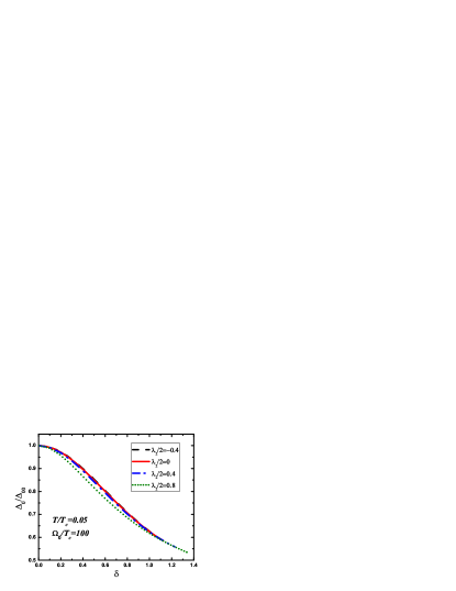
Figure 3: Gap amplitude as a function of the gap anisotropy for Model B at low temperature. The BCS value $\Delta_{00}=2.14k_{B}T_{c}$. Note the smooth evolution of the gap amplitude across the value $\delta=1$, where a horizontal line of nodes appears.

VI.2 Thermal conductivity

We use Eq.(11) with $\Delta=\Delta_{0}[1+\delta\cos\chi_{z}]\cos 2\phi$ to evaluate the temperature dependence of the thermal conductivity in a quasi-two dimensional superconductor. For our calculations we used the impurity scattering in the unitarity limit, with the normal state $\Gamma_{N}=0.007T_{c}$. While both $\kappa_{zz}$ and $\kappa_{xx}$ show the standard dependence on the scattering rate for unconventional superconductors Graf et al. (1996), the anisotropy ratio is essentially insensitive to impurity concentration in the clean limit $\Gamma_{N}\ll T_{c}$. The results are shown in Figs. 4 and 5. One point of note is that the $c$-axis thermal conductivity is even in $\delta$, while the in-plane transport is sensitive to whether the largest or the smallest gap occurs for $k_{z}=0$, where the in-plane Fermi velocity is the greatest, see Eq.(3).

Figure 4: In-plane thermal conductivity for the modulated state.

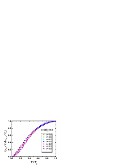
Figure 5: Interplane thermal conductivity for the modulated state.

Of immediate interest to us is the temperature dependence of the anisotropy, $R(T)/R_{n}$, which is shown in Fig. 6. The qualitative understanding of the temperature dependence relies on the observation that the modulation changes the gap most significantly in the regions $\chi_{z}=0,\pm\pi$, where the quasiparticle velocity is strictly in the ab plane, with no component along the $c$-axis. Consequently, for $\delta>0$ the in-plane conductivity is reduced compared to that of a superconductor with an unmodulated gap, while for $\delta<0$ it is increased. As a result, for $\delta>0$ the anisotropy ratio $\kappa_{zz}/\kappa_{xx}$ below $T_{c}$ is enhanced compared to the normal state value, while for $\delta<0$ it is reduced. Notice that for our model $\kappa_{zz}$ is insensitive to the sign of $\delta$ since points at the Fermi surface where $\cos\chi_{z}=\pm a$ ($\chi_{z}=\alpha,\pi-\alpha$) have identical values of the Fermi velocity, and therefore contribute equally to the $c$-axis thermal conductivity.

The residual anisotropy in the $T\rightarrow 0$ limit can be computed analytically once we recognize that, prior to integration over the $z$-component of the momentum, for each value of $\chi_{z}$ the contribution of the kernel to the conductivity is universal in complete analogy to a two-dimensional $d$-wave superconductor with the gap $\Delta(\chi_{z})$. Consequently, the ratio of the residual low temperature terms is ($\lambda=2t/E_{F}$)

$$\frac{R_{0}}{R_{n}} = 2\left[\int_{-\pi}^{\pi}\frac{\sin^{2}(\chi_{z})d\chi_{z}}{1+\delta\cos\chi_{z}}\right]/\left[\int_{-\pi}^{\pi}\frac{(1+\lambda\cos(\chi_{z}))d\chi_{z}}{1+\delta\cos\chi_{z}}\right]$$ (27)

$$= 2\frac{1-\sqrt{1-\delta^{2}}}{\delta^{2}}\left[\frac{\lambda}{\delta}+\left(1-\frac{\lambda}{\delta}\right)\frac{1}{\sqrt{1-\delta^{2}}}\right]^{-1}.$$

This result is shown in Fig. 6. The experimentally determined $R_{s}(T)/R_{0}$ is as low as 0.5 at temperatures of the order of 0.2T_c Shakeripour et al. (2006). This can only be achieved for large negative values of the gap anisotropy, $|\delta|=-\delta\gtrsim 0.8$, when the gap nearly vanishes in the equatorial plane of the Fermi surface. This value is possible for sufficiently strong coupling $\lambda_{1}$, but we consider it not very likely in CeIrIn₅. In this model both $\kappa_{zz}$ and $\kappa_{xx}$ are universal, albeit with different values, and therefore future doping studies of this material will be able to test the universality of the $z$-axis thermal conductivity.

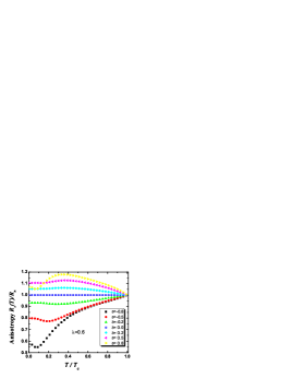
Figure 6: Anisotropy of the thermal conductivity for the model.

VII Model C: modulated interplane hopping

VII.1 Justification and general considerations

In quasi-two dimensional systems the interplane matrix element depends on the overlap of the atomic orbitals contributing to the bands close to the Fermi surface. Therefore, in general, the in-plane and out-of-plane motion of the quasiparticles are coupled, and, in writing the tight-binding ansatz for the open Fermi surface along the c-axis, it is necessary to recognize that the matrix element $t$ is a function of the in-plane direction of the momentum, $\phi$. Moreover, simply looking at the quasi-2D sheet of the Fermi surface of CeIrIn₅ as obtained by band-structure calculations and by dHvA measurements Haga et al. (2001), it is clear that The Fermi surface is not rotationally invariant, and therefore it is necessary to account for the angle-dependence of tunneling. For the Fermi surface of a general shape $k_{F}^{2}=k_{x}^{2}+k_{y}^{2}-2t\cos\chi_{z}$ the difference between the maximal and minimal values of the radius, $k_{0}^{2}(k_{z})$ is $4t$. In the 115 series this difference is greater along the [110] direction than along the [100] direction, which suggest that $t$ is $\phi$-dependent Haga et al. (2001).

In the normal state this dependence does little beyond replacing $t$ with the appropriate average over the directions, see Sec. IV. In a superconducting state with an anisotropic gap, however, the effect of the modulation of the interplane hopping can be much more pronounced. The best studied example is the high-T_c cuprates, where, on the basis of band structure calculations, $t(\phi)$ is expected to vanish along the directions of the nodes in the gap Xiang and Wheatley (1996). Among the manifestations of this effect are the high power law in the temperature variation of the c-axis penetration depth ($T^{5}$ rather than $T$ in the pure limit) Panagopoulos et al. (1997), and weak dependence of the Josephson plasma resonance frequency on temperature at $T\ll T_{c}$  Gaifullin et al. (1999).

In the analysis of the thermal conductivity it is easy to see that any directional dependence $t(\phi)$ results in a deviation of the anisotropy ratio, $R_{s}(T)$, from its normal state value, $R_{n}$, even for a superconducting gap that has pure $d$-wave form, $\Delta=\Delta_{0}\cos 2\phi$, with no $k_{z}$-dependence. This is simply because the quasiparticle velocity, $v_{z}$, now acquires a dependence on the angle $\phi$, which affects the evaluation of the thermal conductivity kernel, $K_{z}$, see Eq.(11). Moreover, since the universal low temperature behavior is due to near-nodal quasiparticles, any suppression of the hopping matrix element in the vicinity of the nodes reduces the contribution of these quasiparticles to the c-axis transport, making it non-universal, while preserving the universality of the low temperature limit for the in-plane conductivity. Therefore assuming a modulated hopping may provide a route towards the explanation of the experimental results.

VII.2 Model and thermal conductivity

Once again we adopt the model energy dispersion of the form

$$\epsilon(\bm{k})=\frac{k_{x}^{2}+k_{y}^{2}}{2m}-2t(\phi)\cos(k_{z}c),$$ (28)

where

$$t(\phi)=t_{0}+t_{1}\cos^{2}2\phi,$$ (29)

which is the simplest anisotropic form satisfying the tetragonal symmetry. This additional $\phi$ dependence does not affect the in-plane thermal conductivity, $\kappa_{xx}$, but does modify the out of plane $\kappa_{zz}$. As discussed in Sec.IV, to a good approximation the normal state anisotropy ratio is

$$R_{n}=\frac{\kappa_{zz}}{\kappa_{xx}}=\left[\frac{t_{0}^{2}}{E_{F}^{2}}+\frac{t_{0}t_{1}}{E_{F}^{2}}+\frac{3}{8}\frac{t_{1}^{2}}{E_{F}^{2}}\right](k_{F}c)^{2}.$$ (30)

For simplicity, and in agreement with the results of the previous section showing that small $c$-axis modulation of the gap does not yield significant corrections to the anisotropy ratio in the superconducting state, we consider a $d$-wave gap in this calculation. In agreement with the discussion above, we are interested in the situation when the interplane transport is suppressed along the nodal directions, and therefore take $\Delta=\Delta_{0}\cos 2\phi$.

Neglecting the small corrections to the in-plane Fermi velocity due to the angle-dependence of $t$, as discussed in Sec.IV, we find

$$K_{x}=\frac{v_{F}^{2}}{\pi\widetilde{\omega}_{1}\widetilde{\omega}_{2}}\>{\rm Re}\left[\widetilde{\omega}\>{\rm E}\left(\frac{\Delta_{0}}{\widetilde{\omega}}\right)+\frac{|\widetilde{\omega}|^{2}-\widetilde{\omega}^{2}}{2\widetilde{\omega}}\>{\rm K}\left(\frac{\Delta_{0}}{\widetilde{\omega}}\right)\right]\;.$$ (31)

The kernel for the interplane conductivity is more complex,

$$K_{z}=\frac{4c^{2}}{\pi\widetilde{\omega}_{1}\widetilde{\omega}_{2}}\>{\rm Re}\Biggl{\{}t_{0}^{2}\left[\widetilde{\omega}\>{\rm E}\left(\frac{\Delta_{0}}{\widetilde{\omega}}\right)+\frac{|\widetilde{\omega}|^{2}-\widetilde{\omega}^{2}}{2\widetilde{\omega}}\>{\rm K}\left(\frac{\Delta_{0}}{\widetilde{\omega}}\right)\right]+2t_{0}t_{1}\left[\widetilde{\omega}\>I_{1e}\left(\frac{\Delta_{0}}{\widetilde{\omega}}\right)+\frac{|\widetilde{\omega}|^{2}-\widetilde{\omega}^{2}}{2\widetilde{\omega}}\>I_{1k}\left(\frac{\Delta_{0}}{\widetilde{\omega}}\right)\right]$$ (32)

$$+t_{1}^{2}\left[\widetilde{\omega}\>I_{2e}\left(\frac{\Delta_{0}}{\widetilde{\omega}}\right)+\frac{|\widetilde{\omega}|^{2}-\widetilde{\omega}^{2}}{2\widetilde{\omega}}\>I_{2k}\left(\frac{\Delta_{0}}{\widetilde{\omega}}\right)\right]\Biggr{\}},$$ (33)

where

$$I_{1e}(x) = \frac{2x^{2}-1}{3x^{2}}E(x)-\frac{x^{2}-1}{3x^{2}}K(x),$$ (34)

$$I_{1k}(x) = \frac{K(x)-E(x)}{x^{2}},$$ (35)

$$I_{2e}(x) = \frac{8x^{4}-3x^{2}-2}{15x^{4}}E(x)+\frac{2(1+x^{2}-2x^{4})}{15x^{4}}K(x),$$ (36)

$$I_{2k}(x) = -\frac{2}{3}\frac{1+x^{2}}{x^{4}}E(x)+\frac{2+x^{2}}{3x^{4}}K(x).$$ (37)

The $T=0$ limit, which is important for the comparison with the universal limit, can also be readily evaluated as a function of the low energy scattering rate, $\gamma$, by setting $\widetilde{\omega}=i\gamma$. We reproduce the standard result for the in-plane conductivity,

$$\lim_{T\rightarrow 0}\frac{\kappa_{xx}}{T}=\frac{\pi}{6}\frac{N_{0}v_{F}^{2}}{\sqrt{\gamma^{2}+\Delta_{0}^{2}}}E\left(\frac{\Delta_{0}}{\sqrt{\gamma^{2}+\Delta_{0}^{2}}}\right),$$ (38)

while for the interplane thermal conductivity we find

$$\lim_{T\rightarrow 0}\frac{\kappa_{zz}}{T}=\frac{2\pi}{3}\frac{N_{0}c^{2}}{\sqrt{\gamma^{2}+\Delta_{0}^{2}}}\Biggl{\{} t_{0}^{2}E\left(\frac{\Delta_{0}}{\sqrt{\gamma^{2}+\Delta_{0}^{2}}}\right)+2t_{0}t_{1}\frac{\gamma^{2}}{\Delta_{0}^{2}}\left[K\left(\frac{\Delta_{0}}{\sqrt{\gamma^{2}+\Delta_{0}^{2}}}\right)-E\left(\frac{\Delta_{0}}{\sqrt{\gamma^{2}+\Delta_{0}^{2}}}\right)\right]$$ (40)

$$+t_{1}^{2}\frac{\gamma^{2}}{\Delta_{0}^{2}}\left[E\left(\frac{\Delta_{0}}{\sqrt{\gamma^{2}+\Delta_{0}^{2}}}\right)-2\frac{\gamma^{2}}{\Delta_{0}^{2}}\left[K\left(\frac{\Delta_{0}}{\sqrt{\gamma^{2}+\Delta_{0}^{2}}}\right)-E\left(\frac{\Delta_{0}}{\sqrt{\gamma^{2}+\Delta_{0}^{2}}}\right)\right]\right]\Biggr{\}}.$$

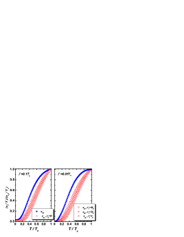
Figure 7: Temperature dependence of the in-plane and the interplane thermal conductivity for the model with modulated hopping. The impurities are assumed to be in the unitarity limit, with $\Gamma$ the normal state scattering rate.

In the clean limit, $\gamma\ll\Delta_{0}$, the residual in-plane conductivity is universal,

$$\lim_{T\rightarrow 0}\frac{\kappa_{xx}}{T}\approx\frac{\pi}{6}\frac{N_{0}v_{F}^{2}}{\Delta_{0}},$$ (41)

while the $c$-axis conductivity, for $t_{0}/t_{1}>\gamma/\Delta_{0}$, is given by

$$\lim_{T\rightarrow 0}\frac{\kappa_{zz}}{T}\approx\frac{2\pi}{3}\frac{N_{0}c^{2}}{\Delta_{0}}t_{0}^{2},$$ (42)

which implies that the residual anisotropy ratio is

$$\frac{R_{0}}{R_{n}}=\left[1+\frac{t_{1}}{t_{0}}+\frac{3t_{1}^{2}}{8t_{0}^{2}}\right]^{-1}<1.$$ (43)

Even for a very moderate anisotropy ratio, $t_{1}/t_{0}=2$ (which, for samples with $\gamma/\Delta_{0}\sim 0.1$ is well within the range of the approximation), the anisotropy ratio at low temperature is already low at about 22%.

The reduction of the anisotropy is even more pronounced for the cases of extreme anisotropy, $t_{0}/t_{1}\ll\gamma/\Delta$, when

$$\frac{R_{0}}{R_{n}}\approx\frac{8}{3}\frac{\gamma^{2}}{\Delta_{0}^{2}}\left[1+\frac{t_{0}}{t_{1}}\ln\frac{4\Delta_{0}}{e\gamma}\right]\ll 1.$$ (44)

Consequently in this model the residual anisotropy ratio can be arbitrarily small depending on the purity. If there are no symmetry requirements for the hopping matrix element to vanish for the nodal directions, in most situations we do not expect $t_{0}$ and $t_{1}$ to differ by an order of magnitude; this suggests that the residual linear term is visible in the $c$-axis thermal conductivity, but may be significantly smaller than its in-plane counterpart. While the results above give a rough estimate of the effect of impurities on the residual anisotropy, it is worth noting that disorder is likely to make the interplane hopping more isotropic, and therefore tends to restore the anisotropy to the the normal state value faster that what Eq.(44) indicates.

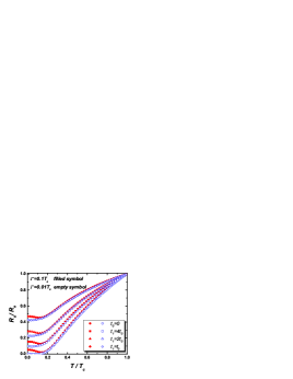
Figure 8: Temperature dependence of the anisotropy of the interplane to the intraplane thermal conductivity. Note that the residual value is increasing with increasing $t_{0}/t_{1}$.

VIII Model D: hybrid gap

So far we looked at the models with vertical line nodes, motivated by possible similarities between CeIrIn₅ and CeCoIn₅, and attempted to reconcile them with the experimental measurements. Of course, in the absence of any information about the nodal structure, a natural explanation for the observed anisotropy is that, in analogy to UPt₃, the system has a horizontal line of nodes, and therefore the nodal quasiparticles do not contribute to the $c$-axis transport. We consider this model now.

The hybrid gap belongs to the representation that transforms as $\widehat{k}_{z}(\widehat{k}_{x}\pm i\widehat{k}_{y})$. The basis function for this representation over an open Fermi surface is $(k_{x}\pm ik_{y})\sin\chi_{z}$, and therefore, for, if we take the weakly modulated limit, $k_{F,x}^{2}+k_{F,y}^{2}\approx$const, the gap amplitude is $|\Delta(\chi_{z},\phi)|=\Delta_{0}|\sin\chi_{z}|$. If we take into account the fourfold, rather than cylindrical, shape of the Fermi surface, there may be additional small modulation of this gap with the component of the Fermi momentum in the $xy$ plane as a function of $z$: based on our results for Model B in Sec.VI, we ignore these. Then the density of states, and the in-plane thermal conductivity for this model are identical to that for a system with vertical line nodes, while the interplane thermal conductivity kernel is given by

$$K_{z}=\frac{4t^{2}c^{2}}{\pi\widetilde{\omega}_{1}\widetilde{\omega}_{2}}\>{\rm Re}\left[\widetilde{\omega}\>I_{1e}\left(\frac{\Delta_{0}}{\widetilde{\omega}}\right)+\frac{|\widetilde{\omega}|^{2}-\widetilde{\omega}^{2}}{2\widetilde{\omega}}\>I_{1k}\left(\frac{\Delta_{0}}{\widetilde{\omega}}\right)\right]$$ (45)

The temperature dependence of $\kappa_{xx}$ and $\kappa_{zz}$ is shown in Fig. 9, and the corresponding anisotropy ratio for the hybrid gap is given in Fig. 10 for the hybrid gap for different values of the impurity scattering. At low $T$ the in-plane thermal conductivity is universal, while the interplane conductivity,

$$\lim_{T\rightarrow 0}\frac{\kappa_{zz}}{T} \approx \frac{2\pi}{3}\frac{N_{0}t^{2}c^{2}}{\sqrt{\gamma^{2}+\Delta_{0}^{2}}}$$

$$\times\frac{\gamma^{2}}{\Delta_{0}^{2}}\left[K\left(\frac{\Delta_{0}}{\sqrt{\gamma^{2}+\Delta_{0}^{2}}}\right)-E\left(\frac{\Delta_{0}}{\sqrt{\gamma^{2}+\Delta_{0}^{2}}}\right)\right]$$

$$\approx \frac{2\pi}{3}\frac{N_{0}t^{2}c^{2}}{\Delta_{0}}\frac{\gamma^{2}}{\Delta_{0}^{2}}\ln\frac{4\Delta_{0}}{e\gamma},$$ (47)

gives the residual anisotropy

$$\frac{R_{0}}{R_{n}}\approx\frac{\gamma^{2}}{\Delta_{0}^{2}}\ln\frac{4\Delta_{0}}{e\gamma}.$$ (48)

This result is clearly non-universal. Notice that the dependence on the impurity scattering here differs from the $\gamma/\Delta_{0}$ result obtained for UPt₃ in Ref. Norman and Hirschfeld, 1996. The reason for the discrepancy is that for the hybrid gap and a Fermi surface closed along the $c$-axis the quasiparticles contributing the most to the $c$-axis conductivity are near the north and south pole. For the open Fermi surface these quasiparticles are absent, and the $c$-axis conductivity is reduced by an additional factor of $\gamma/\Delta_{0}$. It is also obvious, from comparing this with the results of the previous section, that the residual anisotropy can be close for the models C and D, and may not provide the unequivocal distinction between the two.

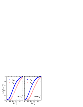
Figure 9: Temperature dependence of the in-plane and the interplane thermal conductivity for the hybrid gap. The impurities are assumed to be in the unitarity limit, with $\Gamma$ the normal state scattering rate.

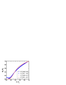
Figure 10: Temperature dependence of the anisotropy of the interplane to the intraplane thermal conductivity for the hybrid gap. For comparison, we include results with deviations from the unitarity scattering limit.

IX Discussion.

It follows from experiment that the low-$T$ value of the anisotropy of the thermal conductivity is below 25% of the normal value. The analysis above shows that model A (simple $d$-wave with constant interplane coupling) does not give results that can explain the observed anisotropy. Model B (weakly modulated, along the $c$-axis, amplitude of the $d$-wave gap) shows some tendency towards the temperature-dependent anisotropy, but, in our view, requires fine tuning if it were to explain the measurements of Ref. Shakeripour et al., 2006. On the other hand, both model C (modulated interlayer hopping, vertical line nodes) and model D (horizontal line nodes) give very similar behavior of the thermal conductivity as a function of temperature, with a low residual value of the anisotropy $\kappa_{c}/\kappa_{a}$, and therefore may be relevant to CeIrIn₅. Distinguishing between the two based purely on the thermal conductivity data may not be easy, as is seen from the comparison in Fig.11, which shows that, for sufficiently high anisotropy of $t_{1}/t_{0}$, there is essentially no difference in the behavior of the ratio $\kappa_{c}/\kappa_{a}$ as a function of temperature between the two models.

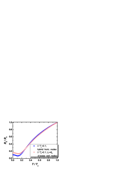
Figure 11: Comparison of the temperature dependence for the hybrid and the d-wave gap.

There are notable differences between the results presented for either model and the experimental observations of Ref. Shakeripour et al., 2006. In experiment, the anisotropy ratio does not decrease below 0.5 for temperatures as low as 0.1$T_{c}$, and there is no sign of saturation of the ratio below 0.15$T_{c}$ as in theoretical analysis. This is due to strong inelastic scattering that results in a peak in $\kappa_{c}/\kappa_{a}$ at about $0.3T_{c}$, but which is not included in our analysis here. Correspondingly, the low-$T$ fit to experiment is done just below the peak, and the rapid decrease of the anisotropy may be related to the inelastic scattering.

The low residual value of the thermal conductivity anisotropy implies, in model C, highly anisotropic tunneling, $t_{1}\geq 2t_{0}$. Published band structure data do not allow to reliably extract this ratio from fitting the quasi-two dimensional sheet of the Fermi surface, but this is the task that perhaps should be attempted in near future. In the meantime, we propose several experiments that have the potential to provide additional information to resolve the question of vertical vs. horizontal line nodes.

1. Direct measurement of the specific heat and/or thermal conductivity in the vortex state under a rotated applied field. This is, in our view, the best test for the existence of the line nodes. If, for the field rotated in the $xy$ plane, no difference in the specific heat is found across the $H$-$T$ phase diagram for the field direction along [110] vs. [100] direction, it is likely that there no vertical lines of nodes. If, on the other hand, such anisotropy is found and develops in agreement with theoretical predictions Vekhter et al. (1999); Vorontsov and Vekhter (2006), this would be a strong evidence for $d$-wave, rather than hybrid, gap.

   At the same time, it is possible, although, in our view, unlikely, that there is gap modulation both in the plane and along the $c$-axis. Therefore measurements of the specific heat and thermal conductivity when the field is rotated in the $zy$ or $xz$ plane should be used to eliminate this possibility, and directly probe for horizontal line nodes. Low superconducting transition temperature of CeIrIn₅ and inelastic scattering require that these measurements be done at temperatures below $\sim$150mK.

2. Measurement of the $c$-axis thermal conductivity in CeCoIn₅. In the Co compound there is a general agreement that there are vertical line nodes. Measurements of the temperature evolution of the anisotropy $\kappa_{c}/\kappa_{a}$ in that compound, and comparison with CeIrIn₅, while short of proof, would provide a test for the connection between the anisotropy and the location of the nodes. Note that there is some evidence for remaining unpaired electrons in the superconducting state of CeCoIn₅ (at least upon La-doping) Tanatar et al. (2005), which leads to a residual metallic linear term for both directions of the heat current. However, as it was suggested that the fraction of these quasiparticles can be determined experimentally Tanatar et al. (2005), their contribution can be subtracted, and the remaining anisotropy used to test the differences and similarities between CeCoIn₅ and CeIrIn₅.

3. $c$-axis penetration depth measurements. In analogy to cuprates, if the interplane transport is suppressed along the nodal directions, the $c$-axis penetration depth should either be not linear in $T$ at $T\ll T_{c}$ (for $t_{1}\gg t_{0}$) or have a small range of linear $T$ behavior, with the coefficient much smaller than that inferred from the density of states varying as $E/\Delta_{0}$. In CeCoIn₅ the $c$-axis penetration depth is linear in $T$, and observation of the non-linear behavior in CeIrIn₅ would point towards differences between the two systems. Unfortunately, we expect that, for reasons similar to those outlines for the thermal conductivity, it would be difficult to distinguish model C from model D on the basis of this measurement. Negative result, however (linear, in $T$, $\lambda_{c}(T)$) would be difficult to reconcile with the thermal conductivity measurements.

4. Doping studies of residual $c$-axis thermal conductivity in CeIrIn₅. In Fig.12 we show the evolution of the residual thermal conductivity along the $c$-axis, in units of the expected universal value for that direction, as a function of the low-energy scattering rate, $\gamma$. Notice that the increase in $\kappa_{zz}/T$ for the hybrid gap is slow, while for the modulated interplane hopping of model C it is faster. In reality we expect that addition of impurities will tend to make the interplane hopping more isotropic in addition to introducing pairbreaking, and therefore the increase in the residual value of $\kappa_{zz}/T$ will be even faster than that suggested by Fig.12. We therefore predict that, if model C of vertical line nodes with modulated $t$ is realized, disordering the sample will produce a much more pronounced effect on the interplane thermal conductivity than that suggested by a hybrid gap.

   

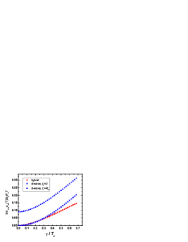
   Figure 12: Increase of the residual thermal conductivity with impurity scattering rate.

X Conclusions

In conclusion, we investigated the constraints placed on the shape of the superconducting gap in CeIrIn₅ by the results of Shakeripour et al Shakeripour et al. (2006), assuming a one-band model with the Fermi surface open along the $c$-axis of the crystal. We find that the temperature evolution of the anisotropy between the transport along the $c$-axis and in the plane is incompatible with a simple $d$-wave gap over a quasi-two dimensional Fermi surface, such as often assumed in the studies of related compound, CeCoIn₅. The temperature variation of the anisotropy shows that the $c$-axis conductivity is affected more significantly than its intraplane counterpart by the opening of the superconducting gap. This implies that the ability of the unpaired quasiparticles to carry heat current along the $c$-axis is impaired relative to their contribution to the in-plane transport. This disparity can arise either from the gap anisotropy or the Fermi surface properties. We explored several models where such modulation has different physical origin.

We find that a weakly $c$-axis modulated $d$-wave gap does not easily provide satisfactory agreement with experiment, although may do so with fine tuning of the parameters. Of the models with constant interplane hopping, that with horizontal line nodes most naturally account for the anisotropy, in partial agreement with the argument of Shakeripour et al.

Remarkably, we also find that an alternative model, where the $c$-axis hopping depends on the direction of the in-plane quasiparticle momentum, yield results that agree with the experimental data even if purely $d$-wave gap, with vertical line nodes, is assumed. Such an agreement requires substantial variation of the hopping between the nodal and the antinodal directions, in qualitative agreement with the analysis of the Fermi surface obtained in the dHvA measurements.

Given that there is some evidence for a distinct superconducting dome in CeIrIn₅ it is clearly very important to determine the shape of the gap. We therefore suggested several possible experiments aimed directly at distinguishing the two situations and hope that further analysis will help resolve the uncertainty regarding the gap symmetry in this material. We also believe that the analysis above is generally relevant to a number of unconventional superconductors with a quasi-two-dimensional parts of the Fermi surface.

XI Acknowledgements

We are very indebted to H. Shakeripour and L. Taillefer for discussing their results with us before publication, and to M. A. Tanatar for correspondence. We are also grateful to C. Capan for critical reading of the manuscript. This research was supported in part by the Board of Regents of Louisiana.

References

- Blount (1985) E. I. Blount, Phys. Rev. B 32, 2935 (1985).
- Volovik and Gor’kov (1985) G. E. Volovik and L. P. Gor’kov, Zh. Eksp. Teor. Fiz. 88, 1412 88, 1412 (1985), [Sov. Phys. JETP 61, 843 (1985)].
- Sigrist and Ueda (1991) M. Sigrist and K. Ueda, Rev. Mod. Phys. 63, 239 (1991).
- Lee (1993) P. A. Lee, Phys. Rev. Lett. 71, 1887 (1993).
- Sun and Maki (1995) Y. Sun and K. Maki, Europhys. Lett. 32, 355 (1995).
- Graf et al. (1996) M. J. Graf, S.-K. Yip, J. A. Sauls, and D. Rainer, Phys. Rev. B 53, 15147 (1996).
- Durst and Lee (2000) A. C. Durst and P. A. Lee, Phys. Rev. B 62, 1270 (2000).
- Taillefer et al. (1997) L. Taillefer, B. Lussier, R. Gagnon, K. Behnia, and H. Aubin, Phys. Rev. Lett. 79, 483 (1997).
- Chiao et al. (2000) M. Chiao, R. W. Hill, C. Lupien, L. Taillefer, P. Lambert, R. Gagnon, and P. Fournier, Phys. Rev. B 62, 3554 (2000).
- Yu et al. (1995) F. Yu, M. B. Salamon, A. J. Leggett, W. C. Lee, and D. M. Ginsberg, Phys. Rev. Lett. 74, 5136 (1995).
- Aubin et al. (1997) H. Aubin, K. Behnia, M. Ribault, R. Gagnon, and L. Taillefer, Phys. Rev. Lett. 78, 2624 (1997).
- Izawa et al. (2003) K. Izawa, Y. Nakajima, J. Goryo, Y. Matsuda, S. Osaki, H. Sugawara, H. Sato, P. Thalmeier, and K. Maki, Phys. Rev. Lett. 90, 117001 (2003).
- Izawa et al. (2002a) K. Izawa, K. Kamata, Y. Nakajima, Y. Matsuda, T. Watanabe, M. Nohara, H. Takagi, P. Thalmeier, and K. Maki, Phys. Rev. Lett. 89, 137006 (2002a).
- Watanabe et al. (2004) T. Watanabe, K. Izawa, Y. Kasahara, Y. Haga, Y. Onuki, P. Thalmeier, K. Maki, and Y. Matsuda, Phys. Rev. B 70, 184502 (2004).
- Izawa et al. (2001) K. Izawa, H. Yamaguchi, Y. Matsuda, H. Shishido, R. Settai, and Y. Onuki, Phys. Rev. Lett. 87, 057002 (2001).
- Izawa et al. (2002b) K. Izawa, H. Yamaguchi, T. Sasaki, and Y. Matsuda, Phys. Rev. Lett. 88, 027002 (2002b).
- Arfi et al. (1989) B. Arfi, H. Bahlouli, and C. J. Pethick, Phys. Rev. B 39, 8959 (1989).
- Fledderjohann and Hirschfeld (1995) A. Fledderjohann and P. J. Hirschfeld, Solid State Communications 94, 163 (1995).
- Lussier et al. (1994) B. Lussier, B. Ellman, and L. Taillefer, Phys. Rev. Lett. 73, 3294 (1994).
- Norman and Hirschfeld (1996) M. R. Norman and P. J. Hirschfeld, Phys. Rev. B 53, 5706 (1996).
- Shakeripour et al. (2006) H. Shakeripour, M. A. Tanatar, S. Y. Li, L. Taillefer, and C. Petrovic (2006), eprint cond-mat/0610052.
- Aoki et al. (2004) H. Aoki, T. Sakakibara, H. Shishido, R. Settai, Y. Onuki, P. Miranović, and K. Machida, J. Physics: Condensed Matter 16, L13 (2004).
- Nicklas et al. (2004) M. Nicklas, V. A. Sidorov, H. A. Borges, P. G. Pagliuso, J. L. Sarrao, and J. D. Thompson, Phys. Rev. B 70, 020505 (2004).
- Haga et al. (2001) Y. Haga, Y. Inada, H. Harima, K. Oikawa, M. Murakawa, H. Nakawaki, Y. Tokiwa, D. Aoki, H. Shishido, S. Ikeda, et al., Phys. Rev. B 63, 060503 (2001).
- Bianchi et al. (2003) A. Bianchi, R. Movshovich, I. Vekhter, P. G. Pagliuso, and J. L. Sarrao, Phys. Rev. Lett. 91, 257001 (2003).
- Paglione et al. (2003) J. Paglione, M. A. Tanatar, D. G. Hawthorn, E. Boaknin, R. W. Hill, F. Ronning, M. Sutherland, L. Taillefer, C. Petrovic, and P. C. Canfield, Phys. Rev. Lett. 91, 246405 (2003).
- Kohori et al. (2001) Y. Kohori, Y. Yamato, Y. Iwamoto, T. Kohara, E. D. Bauer, M. B. Maple, and J. L. Sarrao, Phys. Rev. B 64, 134526 (2001).
- Zheng et al. (2001) G.-q. Zheng, K. Tanabe, T. Mito, S. Kawasaki, Y. Kitaoka, D. Aoki, Y. Haga, and Y. Onuki, Phys. Rev. Lett. 86, 4664 (2001).
- Movshovich et al. (2001) R. Movshovich, M. Jaime, J. D. Thompson, C. Petrovic, Z. Fisk, P. G. Pagliuso, and J. L. Sarrao, Phys. Rev. Lett. 86, 5152 (2001).
- Chia et al. (2003) E. E. M. Chia, D. J. V. Harlingen, M. B. Salamon, B. D. Yanoff, I. Bonalde, and J. L. Sarrao, Phys. Rev. B 67, 014527 (2003).
- Park et al. (2005) W. K. Park, L. H. Greene, J. L. Sarrao, and J. D. Thompson, Phys. Rev.B 72, 052509 (2005).
- Xiang and Wheatley (1996) T. Xiang and J. M. Wheatley, Phys. Rev. Lett. 77, 4632 (1996).
- Gaifullin et al. (1999) M. B. Gaifullin, Y. Matsuda, N. Chikumoto, J. Shimoyama, K. Kishio, and R. Yoshizaki, Phys. Rev. Lett. 83, 3928 (1999).
- Panagopoulos et al. (1997) C. Panagopoulos, J. R. Cooper, T. Xiang, G. B. Peacock, I. Gameson, and P. P. Edwards, Phys. Rev. Lett. 79, 2320 (1997).
- Hosseini et al. (1998) A. Hosseini, S. Kamal, D. A. Bonn, R. Liang, and W. N. Hardy, Phys. Rev. Lett. 81, 1298 (1998).
- Kübert and Hirschfeld (1998) C. Kübert and P. J. Hirschfeld, Phys. Rev. Lett. 80, 4963 (1998).
- Allen (1976) P. B. Allen, Phys. Rev. B 13, 1416 (1976).
- Bulaevskii and Zyskin (1990) L. N. Bulaevskii and M. V. Zyskin, Phys. Rev. B 42, 10230 (1990).
- Rajagopal and Jha (1996) A. K. Rajagopal and S. S. Jha, Phys. Rev. B 54, 4331 (1996).
- Jha and Rajagopal (1997) S. S. Jha and A. K. Rajagopal, Phys. Rev. B 55, 15248 (1997).
- Vekhter et al. (1999) I. Vekhter, P. J. Hirschfeld, E. J. Nicol, and J. P. Carbotte, Phys. Rev. B 59, R9023 (1999).
- Vorontsov and Vekhter (2006) A. Vorontsov and I. Vekhter, Phys. Rev. Lett. 96, 237001 (2006).
- Tanatar et al. (2005) M. A. Tanatar, J. Paglione, S. Nakatsuji, D. G. Hawthorn, E. Boaknin, R. W. Hill, F. Ronning, M. Sutherland, L. Taillefer, C. Petrovic, et al., Phys. Rev. Lett. 95, 067002 (2005).