Intermediate dynamics between Newton and Langevin

Abstract

A dynamics between Newton and Langevin formalisms is elucidated within the framework of the generalized Langevin equation. For thermal noise yielding a vanishing zero-frequency friction the corresponding non-Markovian Brownian dynamics exhibits anomalous behavior which is characterized by ballistic diffusion and accelerated transport. We also investigate the role of a possible initial correlation between the system degrees of freedom and the heat-bath degrees of freedom for the asymptotic long-time behavior of the system dynamics. As two test beds we investigate (i) the anomalous energy relaxation of free non-Markovian Brownian motion that is driven by a harmonic velocity noise and (ii) the phenomenon of a net directed acceleration in noise-induced transport of an inertial rocking Brownian motor.

I introduction

The phenomenon of Brownian motion has assumed a fundamental and influential role in the development of thermodynamical and statistical theories and continues to do so as an inspiring source for active research in various fields of natural sciences HM2005 . The Brownian motion dynamics can conveniently be described by a generalized Langevin equation (GLE). The GLE was originally derived by Mori mori1965 , Kawasaki kawasaki73 , and Zwanzig zwanzig by use of the Gram-Schmidt procedure. It was further investigated by Lee using the recurrence relations method lee2 . Starting out from the well-known system-plus-oscillator-reservoir model as e.g. detailed in Ref. zwanzig ; HALNP , one obtains the GLE derived from first principles. The validity of a thermal GLE is typically restricted to the case with a thermal equilibrium; e.g. see in Refs. HALNP ; kubo ; toda ; pot . Specifically, such a GLE dynamics reads kawasaki73 ; zwanzig ; HALNP :

$$m\dot{v}(t)+m\int_{0}^{t}\gamma(t-t^{\prime})v(t^{\prime})dt^{\prime}+\partial_{x}U(x,t)=\varepsilon(t).$$ (1)

Notably, the thermal noise $\varepsilon(t)$ is not correlated with the initial velocity, i.e., $\langle v(0)\varepsilon(t)\rangle=0$, see in Refs. zwanzig ; HALNP and in section III below. In contrast, the initial position $x(0)$ typically is correlated with $\varepsilon(t)$. The memory friction $\gamma(t-t^{\prime})$ is in thermal equilibrium related to the correlation of stationary random forces kubo ; toda . Kubo kubo has addressed the common behavior of a classical equilibrium bath by setting $\langle\varepsilon(t)\varepsilon(t^{\prime})\rangle=mk_{B}T\gamma(t-t^{\prime})$. Here $k_{B}$ is the Boltzmann constant and $T$ denotes the bath temperature. The one-sided Fourier transform of $\gamma(t)$ obeys Re$\tilde{\gamma}(\omega)\geq 0$ for real-valued $\omega$. This correlation result for the thermal noise $\varepsilon(t)$ is commonly termed the fluctuation-dissipation theorem (FDT) of the second kind toda . The nonlinear GLE can also be extended to account for a nonlinear system - linear bath interaction zwanzig ; HALNP ; Illuminati , yielding a structure as in Eq. (1), but now with a nonlinear, coordinate-dependent friction function. It even can be generalized to arbitrary nonlinear system - nonlinear bath interactions containing then the potential of mean force GHT80 .

With this work we aim at extending the theory of classical Brownian motion by focussing on the intricacies of a possible non-Markovian with an incomplete, non-Stokesian dissipative dynamics mor ; vai ; lee ; lutz ; mok ; rubi ; Dhar06 . We will demonstrate that the commonly stated conditions for the equilibrium bath are generally not complete within the framework of linear response theory. This is so, because the existence of anomalous diffusion has not been considered in the original treatment by Kubo and others. Moreover, we discuss also the influence of initial correlation preparation between the system and the heat bath upon the asymptotical behavior of the force-free system.

II Biasing generalized Brownian motion

Let us first consider a free Brownian dynamics with $U(x,t)=0$, possessing via the FDT of the second kind a finite-valued zero-frequency friction. If this dynamics is next subjected to a constant external force, i.e. $-\partial U(x,t)/\partial x=F$, the acceleration vanishes in the case of a Stokesian friction, because the external force balances the friction force. A problem of broad interest is whether there exists an intermediate situation between the Newtonian mechanics and such an ordinary Langevin formalism. This in turn necessitates a non-Stokesian dissipation mechanism such that the asymptotic long-time statistical probability will typically approach a stationary state that explicitly depends on the initial preparation. It is thus of great practical interest to research what kind of heat bath can take on this role. Such non-ergodic non-equilibrium thermodynamics presents a timely subject that is presently hotly debated, both within theory mor ; vai ; lee ; lutz ; Muk2005 ; lee2006 ; Bai2005 and experiment Kutnjak99 ; Fahri99 ; Brok03 .

For a GLE subjected to a constant force; i.e. $U(x,t)=-Fx$, the solution of (1) can be written as

$$x(t) = x(0)+v(0)H(t)+\frac{1}{m}\int^{t}_{0}dt^{\prime}H(t-t^{\prime})(\varepsilon(t^{\prime})+F),$$

$$v(t) = v(0)h(t)+\frac{1}{m}\int^{t}_{0}dt^{\prime}h(t-t^{\prime})(\varepsilon(t^{\prime})+F),$$ (2)

where $H(0)=0$ and $h(0)=1$. The two response functions $H(t)$ and $h(t)$ are the inverse of the Laplace transforms $\hat{H}(s)=[s^{2}+s\hat{\gamma}(s)]^{-1}$ and $\hat{h}(s)=[s+\hat{\gamma}(s)]^{-1}$, respectively, where $\hat{\gamma}(s)$ is the Laplace transform of memory friction kernel, i.e. $\hat{\gamma}(s)=\int^{\infty}_{0}\gamma(t)\exp(-st)dt$. Under the assumption that the characteristic equation $s+\hat{\gamma}(s)=0$ possesses a zero root, i.e. $s=0$, the residue theorem implies that $h(t)=b+\sum_{i}\textmd{res}[\hat{h}(s_{i})]\exp(s_{i}t)$ and $H(t)=c+bt+\sum_{i}s^{-1}_{i}\textmd{res}[\hat{h}(s_{i})]\exp(s_{i}t)$. Here, $s_{i}$ (Re$s_{i}<0$) denote the non-zero roots of the above characteristic equation and res[$\cdots$] are the residues. Within this context, the two relevant, generally non-vanishing quantities $b$ and $c$ are determined to read:

$$b=\frac{1}{1+\hat{\gamma}^{\prime}(0)},\quad c=-\frac{1}{2}b^{2}\hat{\gamma}^{\prime\prime}(0).$$ (3)

This result then requires that $\hat{\gamma}(0)=\int^{\infty}_{0}\gamma(t)dt=0$, i.e., implying a vanishing effective friction at zero frequency.

The average velocity and the average displacement under the external bias $F$ emerge at long times as

$$\{\langle v(t\to\infty)\rangle\} = b\left(\{v(0)\}+\frac{F}{m}t\right)+\frac{F}{m}c,$$ (4)

$$\{\langle x(t\to\infty)\rangle\} = \{x(0)\}+b\left(\{v(0)\}t+\frac{1}{2}\frac{F}{m}t^{2}\right)$$ (5)

$$+ c\left(\{v(0)\}+\frac{F}{m}t\right)+\frac{F}{m}d,$$

where $d=-\sum_{i}\textmd{res}[\hat{h}(s_{i})]/s^{2}_{i}$ is a noise-dependent quantity. Herein, we indicate by $\{\cdots\}$ the average with respect to the initial preparation of the state variables, i.e. an average over their initial values and $\langle\cdots\rangle$ is the noise average. The dissipative acceleration of a Brownian particle of mass $m$ subjected to a constant force $F$ then reads:

$$a=\frac{F}{m}b,$$ (6)

where generally $0\leq b\leq 1$. This quantity $b$ will be termed the dissipation reducing factor, the dissipation is reduced as $b$ is increased. This result is intermediate between a purely Newtonian mechanics (obeying $b=1$) and an ordinary Langevin dynamics (with $b=0$) including of GLEs.

The two limiting results for the asymptotic dynamics are found to read: (i) The Newton case with $b=1$ implying no dissipation, i.e. $\gamma(t)\equiv 0$ with $c=d=0$, yielding: $a=F/m$, $v(t)=v(0)+\frac{F}{m}t$, and $x(t)=x(0)+v(0)t+\frac{1}{2}\frac{F}{m}t^{2}$. (ii) The commonly known, ordinary Langevin situation is obtained with $b=0$; i.e. Eq. (3) then looses validity because of $\hat{\gamma}(0)\neq 0$. For this case $c=\hat{\gamma}^{-1}(0)$ where $\hat{\gamma}(0)$ denotes the Markovian friction strength, resulting in $a=0$, $\langle v(t\to\infty)\rangle=F/(m\hat{\gamma}(0))$, and $\{\langle x(t\to\infty)\rangle\}=\{x(0)\}+\{v(0)\}/\hat{\gamma}(0)+\frac{F}{m}t/\hat{\gamma}(0)+\frac{F}{m}d$.

In the unbiased case, we derive the two-time velocity correlation function (VCF) of free generalized Brownian motion in a generic form, i.e.,

$$\{\langle v(t_{1})v(t_{2})\rangle\} = \frac{k_{B}T}{m}h(|t_{1}-t_{2}|)+\left(\{v^{2}(0)\}-\frac{k_{B}T}{m}\right)$$ (7)

$$h(t_{1})h(t_{2}).$$

Here we used only the condition: $\langle v(0)\varepsilon(t)\rangle=0$. Note that depending on the specific choice for the initial preparation this velocity correlation generally is not time-homogeneous. The stationary velocity correlation function becomes again only a function of $|t_{1}-t_{2}|$ for the case that we use the equilibrium preparation with an initial velocity variance in accordance with the thermal equilibrium value, i.e. $\{v^{2}(0)\}=k_{B}T/m$ Bai2005 . The deduced asymptotic stationary VCF then reads: $C_{vv}(\infty)=b\frac{k_{B}T}{m}\neq 0$. This causes a breakdown of the ergodic equilibrium state because of the initial preparation-dependence, which is encoded in the $v(0)$-dependent asymptotic results: $\langle v\rangle_{st}=bv(0)\neq 0$ and $\{\langle v^{2}\rangle\}_{st}=k_{B}T/m+b^{2}(\{v^{2}(0)\}-k_{B}T/m)$.

Likewise, the mean square displacement (MSD) of the force-free particle is written as

$$\{\langle x^{2}(t)\rangle\} = \{x^{2}(0)\}+\{v^{2}(0)\}H^{2}(t)+2\{x(0)v(0)\}H(t)$$ (8)

$$+ \frac{2}{m}\int^{t}_{0}dt^{\prime}H(t-t^{\prime})\{\langle x(0)\varepsilon(t^{\prime})\rangle\}$$

$$+ \frac{k_{B}T}{m}\left(2\int^{t}_{0}H(t^{\prime})dt^{\prime}-H^{2}(t)\right),$$

where the fourth term denotes the effect of initial coupling between system and heat bath. We will discuss the correlation preparation in the following section. Note that here the largest power in the temporal variation of the MSD involves the square of time. The averaged displacement can be related to the MSD via the generalized Einstein relation, reading

$$\kappa_{2}/\mu_{2}(F\rightarrow 0)=k_{B}T_{\textmd{eff}}\;.$$ (9)

The ballistic diffusion coefficient is $\kappa_{2}=\lim_{t\to\infty}\{\langle x^{2}(t)\rangle\}_{F=0}/(2t^{2})$, being related to the increasing rate of linear mobility $\mu_{2}(F\rightarrow 0)=\lim_{t\to\infty}\{\langle x(t)\rangle\}/(Ft^{2})_{F=0}$. Here, this effective temperature formally reads: $T_{\textmd{eff}}:=T+b(m\{v^{2}(0)\}/k_{B}-T)$, where $T$ is the temperature for the common case with $b=0$.

To assure the equilibrium behavior of this generalized Brownian motion the usual condition of Kubo’s FDT of the second kind for the thermal noise must be complemented as follows: Consider the Fourier transform $\tilde{\gamma}(\omega)$ of the memory damping kernel, i.e.,

$$\tilde{\gamma}(\omega)=\hat{\gamma}(s=-i\omega),$$ (10)

The real part of the former quantity is the spectral density of noise. A ballistic diffusion with $b\neq 0$ thus requires that the lowest power of $\hat{\gamma}(s)$ is of first-order in $s$, implying that the lowest power of Re$\tilde{\gamma}(\omega)$ is proportional to $\omega^{2}$ at low frequencies. Therefore, for a genuine thermal noise driven, force-free particle approaching at the equilibrium state the usual conditions must be completed by: $\lim_{s\to 0}(\hat{\gamma}(s)/s)\to\infty$, or $\lim_{\omega\to 0}(\textmd{Re}\tilde{\gamma}(\omega)/\omega^{2})\to\infty$.

III INITIAL CORRELATION BETWEEN SYSTEM AND BATH

Starting from the system-plus-reservoir model, one knows that the coupling between the system and environmental degrees of freedom there exist four kinds of coupling forms which do not involve a renormalization of potential or mass of the system. In these cases the heat bath consists of a set of independent harmonic oscillators with masses $m_{j}$ and oscillation frequencies $\omega_{j}$. Pervious work Bai2005 has shown that the random force is independent of the system variables for the coordinate-velocity coupling. Nevertheless, however, the expression of thermal noise will depend on the initial preparation of system for the coupling between the system coordinate (velocity) and the environmental coordinates (velocities) considered here. To the best of our knowledge, only a small number of prior studies gra ; HT have considered the general consequences of the detailed initial preparation procedure in view of the asymptotic statistical results of the system.

III.1 The coordinate-coordinate coupling

For a bilinear coupling between the system coordinate $x$ and the heat bath’s coordinates $q_{j}$, the total Hamiltonian can be written as:

$$H=\frac{P_{x}^{2}}{2m}+U(x,t)+\sum_{j}\left[\frac{p^{2}_{j}}{2m_{j}}+\frac{1}{2}m_{j}\omega^{2}_{j}\left(q_{j}-\frac{c_{j}}{m_{j}\omega^{2}_{j}}x\right)^{2}\right]\;.$$ (11)

Here and below the momenta of the system and bath’s oscillators are related to $P_{x}=mv$ and $p_{j}=m_{j}\dot{q}_{j}$, respectively, and the set $c_{j}$ denote the coupling constants. The equation of motion of the system obeys the form of the GLE (1) and the thermal noise appearing in Eq. (1) emerges as zwanzig ; HALNP ; Bai2005

$$\varepsilon(t)=-m\gamma(t)x(0)+\xi_{\textmd{bath}}(t),$$ (12)

where $\gamma(t)=\frac{1}{m}\sum_{j}\frac{c^{2}_{j}}{m_{j}\omega^{2}_{j}}\cos\omega_{j}t$ and $\xi_{\textmd{bath}}(t)$ is determined by the initial coordinates and the velocities of the oscillators of the heat bath. The bath part $\xi_{\textmd{bath}}(t)$ of the noise explicitly reads:

$$\xi_{\textmd{bath}}(t)=\sum_{j}c_{j}\left(q_{j}(0)\cos\omega_{j}t+\frac{\dot{q}_{j}(0)}{\omega_{j}}\sin\omega_{j}t\right).$$ (13)

Physically, this thermal noise $\varepsilon(t)$ obeys statistical properties that derive from the canonical, thermal equilibrium distribution of the total, combined system-plus-bath zwanzig ; HALNP ; ros : this thermal noise then again yields a vanishing mean and its correlation obeys the thermal FDT HALNP . The statistical quantities involving noise the system variables are strictly determined by the joint probability gra . The correlation involving initial position of the system and the thermal noise $\varepsilon(t^{\prime})$, i.e., the fourth term in Eq. (8) reads

$$\frac{2}{m}\int^{t}_{0}dt^{\prime}H(t-t^{\prime})\{\langle x(0)\varepsilon(t^{\prime})\rangle\}$$

$$= -2\{x^{2}(0)\}\int^{t}_{0}dt^{\prime}H(t-t^{\prime})\gamma(t^{\prime})$$

$$= -2H(t)\ast\gamma(t)\{x^{2}(0)\}=-2(1-h(t))\{x^{2}(0)\},$$

wherein $``\ast"$ denotes the convolution integral. It reads, $H(t)\ast\gamma(t)=\frac{1}{2\pi i}\int ds\hat{H}(s)\hat{\gamma}(s)\exp(st)=1-\dot{H}(t)=1-h(t)$. Here we have used the relation below Eq. (2), i.e., $\hat{H}(s)\hat{\gamma}(s)=s^{-1}-s\hat{H}(s)$. This contribution assumes a finite value, i.e., $-2(1-b)\{x^{2}(0)\}$ in the long-time limit.

Under the usual assumption that the thermal noise $\varepsilon(t)$ and the initial velocity $v(0)$ of the system are not correlated, we find from Eq. (12) that the initial coordinate of the system must be uncorrelated with its initial velocity for the coordinate-coordinate coupling case, namely, $\{x(0)v(0)\}=0$, being the case for a canonical thermal equilibrium, cf. the Hamiltonian in Eq. (11). Therefore, the third term in Eq. (8) also vanishes. In the following we shall not consider preparations with such initial correlations between the initial coordinate $x(0)$ and the initial velocity $v(0)$.

III.2 The velocity-velocity coupling

For a bi-linear coupling between the system velocity and the velocities of the bath oscillators the total Hamiltonian reads

$$H=\frac{P_{x}^{2}}{2m}+U(x,t)+\sum_{j}\left[\frac{1}{2m_{j}}\left(p_{j}-\frac{d_{j}}{m}P_{x}\right)^{2}+\frac{1}{2}m_{j}\omega^{2}_{j}q_{j}^{2}\right],$$ (15)

where $d_{j}$ denote the corresponding the coupling constants. We can derive again the GLE (1) describing the motion of the system with the thermal noise term now given by

$$\varepsilon(t) = v(0)\sum_{j}\frac{d^{2}_{j}\omega_{j}}{m_{j}}\sin\omega_{j}t$$ (16)

$$+ \sum_{j}d_{j}\omega^{2}_{j}\left[q_{j}(0)\cos\omega_{j}t+\frac{\dot{q}_{j}(0)}{\omega_{j}}\sin\omega_{j}t\right]$$

$$= v(0)m\int^{t}_{0}\gamma(t^{\prime})dt^{\prime}+\xi_{\textmd{bath}}(t),$$

where $\gamma(t)=\frac{1}{m}\sum_{j}\frac{d^{2}_{j}\omega^{2}_{j}}{m_{j}}\cos\omega_{j}t$ and in addition we have: $\{\langle x(0)\xi_{\textmd{bath}}(t)\rangle\}=\{\langle v(0)\xi_{\textmd{bath}}(t)\rangle\}=0$. We require that the FDT of the second kind is obeyed, namely that $\langle\varepsilon(t)\rangle=0$ and $\langle\varepsilon(t)\varepsilon(t^{\prime})\rangle=k_{B}T\gamma(t-t^{\prime})$. This is guaranteed when $\langle q_{j}(0)\rangle=\langle\tilde{\dot{q}}_{j}(0)\rangle=\langle q_{i}(0)\tilde{\dot{q}}_{j}(0)\rangle=0$, $\langle q_{i}(0)q_{j}(0)\rangle=\frac{k_{B}T}{m\omega^{2}_{j}}\delta_{ij}$, and $\langle\tilde{\dot{q}}_{i}(0)\tilde{\dot{q}}_{j}(0)\rangle=\frac{k_{B}T}{m_{j}}\delta_{ij}$, where $\tilde{\dot{q}}_{i}(0)=\dot{q}_{i}(0)-d_{j}/m_{j}v(0)$ Bai2005 .

In the case of velocity-velocity coupling, the fourth term in Eq. (8) vanishes if again $\{x(0)v(0)\}=0$. An additional term emerges, however, for the mean squared displacement (MSD) of the force-free particle due to the thermal noise $\varepsilon(t)$ which now depends on the initial particle velocity $v(0)$. From Eq. (2), we obtain

$$\{\langle x^{2}(t)\rangle\}_{\textmd{add}} = \frac{2}{m}H(t)\int^{t}_{0}dt^{\prime}H(t-t^{\prime})\{\langle v(0)\varepsilon(t^{\prime})\rangle\}$$ (17)

$$= 2H(t)\{v^{2}(0)\}\int^{t}_{0}dt^{\prime}H(t-t^{\prime})\int^{t^{\prime}}_{0}du\gamma(u)$$

$$= 2(t-H(t))H(t)\{v^{2}(0)\}.$$

Indeed, the ballistic diffusion arises also in this case. Notably, an additional contribution to the mean square velocity of the force-free particle [c.f. Eq. (7) at $t_{1}=t_{2}$] emerges in this case. It reads

$$\{\langle v^{2}(t)\rangle\}_{\textmd{add}} = \frac{2}{m}h(t)\int^{t}_{0}dt^{\prime}h(t-t^{\prime})\{\langle v(0)\varepsilon(t^{\prime})\rangle\}$$ (18)

$$= 2\{v^{2}(0)\}h(t)\int^{t}_{0}dt^{\prime}h(t-t^{\prime})\int^{t^{\prime}}_{0}\gamma(u)du$$

$$= 2h(t)(1-h(t))\{v^{2}(0)\},$$

where we have used the inverse Laplace transform of the convolution integral in Eq. (18) by making use of the relation, $\hat{h}(s)\hat{\gamma}(s)=1-s\hat{h}(s)$.

In particular, the mean squared velocity of the force-free particle emerges in the long-time limit as

$$\{\langle v^{2}(t\to\infty)\rangle\} = 2b(1-b)\{v^{2}(0)\}+\frac{k_{B}T}{m}$$ (19)

$$+ \left(\{v^{2}(0)\}-\frac{k_{B}T}{m}\right)b^{2}.$$

This result evidences that the system can not arrive at the equilibrium state for any initial preparation of the particle velocity if $b\neq 0$. Therefore, for the validity of FDT one has to use at initial time a preparation of thermal equilibrium for the system and the heat bath. Nevertheless, one needs not to worry that the noise is uncorrelated with the initial velocity of the system for a common non-Markovian dynamics with $b=0$. Then, the FDT is valid independent of the coupling form between system and bath whenever the effective Markovian damping of the system is finite at zero frequency. This is so because the first and the third term in Eq. (19) vanishes for $b=0$.

IV Test bed for non-Stokesian dissipative dynamics

Given the FDT of the second kind by Kubo we investigate next unbiased, non-Markovian Brownian motion in (1) that is driven by colored noise known as the harmonic velocity noise (HVN) $\varepsilon(t)$ bao2005 , which, however, does not obey the above additional requirements. The HVN itself is produced from a linear Langevin equation, namely,

$$\dot{y}=\varepsilon,\quad\dot{\varepsilon}=-\Gamma\varepsilon-\Omega^{2}y+\xi(t),$$ (20)

where $\xi(t)$ denotes Gaussian white noise of vanishing mean with $\langle\xi(t)\xi(t^{\prime})\rangle=2\eta\Gamma^{2}k_{B}T\delta(t-t^{\prime})$. The coefficient $\eta$ denotes the damping coefficient of the system corresponding to the thermal white noise; $\Gamma$ and $\Omega$ denote the damping and the frequency parameters. The second moments and the cross-variance of $y(0)$ and $\varepsilon(0)$ obey: $\{y^{2}(0)\}=\eta\Gamma\Omega^{-2}k_{B}T$, $\{\varepsilon^{2}(0)\}=\eta\Gamma k_{B}T$, and $\{y(0)\varepsilon(0)\}=0$. The Laplace transformation of the memory damping kernel reads $\hat{\gamma}(s)=\eta\Gamma s/(s^{2}+\Gamma s+\Omega^{2})$ with

$$\textmd{Re}\tilde{\gamma}(\omega)=\frac{\eta\Gamma^{2}\omega^{2}}{(\Omega^{2}-\omega^{2})^{2}+\Gamma^{2}\omega^{2}}\;,$$ (21)

respectively. The latter corresponds to the spectrum of HVN which indeed vanishes identically at zero-frequency. In this case the dissipation reducing factor emerges as $b=(1+\eta\Gamma\Omega^{-2})^{-1}$, and likewise, $c=(1-b)^{2}/\eta$, $d=(1-b)^{2}[(\eta\Gamma)^{-1}-(1-b)\eta^{-2}]$.

Using models with a bi-linear coordinate system-bath coupling the dynamics can be characterized by the spectral density of bath modes, $J(\omega)$, being related to Re$\tilde{\gamma}(\omega)=J(\omega)/m\omega$ HTB ; gra87 ; RI ; chen . Thus, for a weak coupling to a bath, as it can be realized either with optical-like bath modes mor ; RI , broadband colored noise bao2003 , or also for the celebrated case of a black-body radiation field of the Rayleigh-Jeans type for the static friction vanishes. Yet other physical situations that come to mind involve the vortex diffusion in magnetic fields ao , or open system dynamics with a velocity-dependent system-bath coupling for ; Bai2005 ; bao06 ; poll .

The non-Markovian Brownian motion can equivalently be recast as an embedded, higher-dimensional Markovian process. The Fokker-Planck equation (FPE) for the probability density $P(x,v,w,u,y,\varepsilon;t)$ corresponds then to the dynamics of a set of coupled Markovian LEs involving the auxiliary-variables $(w,u,y,\varepsilon)$: It obeys $\partial_{t}P=L_{FP}P$, where $L_{FP}$ is the associated FPE operator; when being formally supplemented here with a nonvanishing potential $U(x,t)$, it explicitly reads:

$$L_{FP} = -v\frac{\partial}{\partial x}-m^{-1}(-U^{\prime}(x,t)+w)\frac{\partial}{\partial v}$$

$$+(\Gamma w+\eta\Gamma v+\Omega^{2}y+u)\frac{\partial}{\partial w}$$

$$-\Omega^{2}(w-\varepsilon)\frac{\partial}{\partial u}+\varepsilon\frac{\partial}{\partial y}$$

$$+(\Gamma\varepsilon+\Omega^{2}y)\frac{\partial}{\partial\varepsilon}+\eta\Gamma^{2}k_{B}T\frac{\partial^{2}}{\partial w^{2}}+\eta\Gamma^{2}k_{B}T\frac{\partial^{2}}{\partial\varepsilon^{2}}.$$

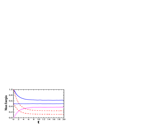
Figure 1: (color online). Behavior of diverse mean energies (see text) for a nonergodic, force-free Brownian particle vs. time $t$. The parameters used are $m=1.0$, $k_{B}T=1.0$, $\eta=0.2$, $\Gamma=5.0$, $\Omega=1.0$, $x(0)=0$, and (i) $v(0)=\sqrt{2}$ and (ii) $1.0$, respectively, for the total energies given by the solid lines and the remnant energies by the dashed lines, from top to bottom. The open circles is the adsorbed energy from the bath for all cases and also the total energy for the $v(0)=0$ case.

IV.1 The energy relaxation

We use this form for the analysis of the energy relaxation. The mean total energy of the thermal HVN-driven force-free particle reads

$$\{\langle E(t)\rangle\} = \frac{1}{2}m\{\langle v^{2}(t)\rangle\}$$

$$= \frac{1}{2}m\{\langle v(t)\rangle^{2}\}+\frac{1}{2}m\{\langle(v(t)-\langle v(t)\rangle)^{2}\rangle\}.$$

The first part describes the remnant initial kinetic energy of the particle, being dissipated partly by the heat bath environment. This part vanishes in the ordinary case with $b=0$. The second part denotes the energy provided from the heat bath. It is independent of the initial particle velocity, but does not relax, however, towards equilibrium. The absorbed power of the particle from the heat bath, namely, the rate of work being done by the fluctuation force li , is

$$P_{\textmd{abs}} = \lim_{t\to\infty}\int^{t}_{0}\gamma(t-t^{\prime})\{\langle v(t)v(t^{\prime})\rangle\}dt^{\prime}$$ (24)

$$= \frac{\eta k_{B}T}{1+\eta/(2\Gamma)+2\Omega^{2}/(\eta\Gamma)}\;.$$

Note that it falls short of the equilibrium value $\eta k_{B}T$. All quantities plotted are dimensionless. Our numerical results are depicted with Fig. 1. These results are obtained via the simulation of a set of Markovian LE’s which are equivalent to the FPE in (22) with $U(x,t)=0$.

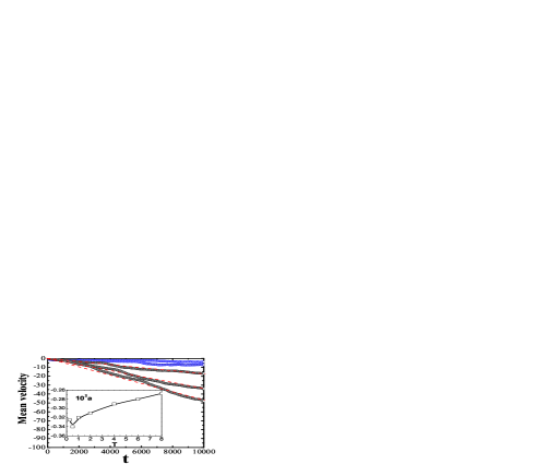
Figure 2: (color online). Accelerated, (time and ensemble)- averaged Brownian motor velocity in a rocking ratchet that is driven by HVN. The used parameters are $x(0)=v(0)=0$, $m=1.0$, $k_{B}T=0.5$, $\eta=5.0$, $\Gamma=22.0$, $\Omega^{2}=40.0$, $t_{p}=25.0$, $A_{0}=2.0$, $4.0$, $6.0$, $10.0$, and $15.0$, from top to bottom. The particles undergo a finite acceleration $a$ (times 100) vs. temperature $T$, being depicted with the inset for $A_{0}=10.0$.

IV.2 Brownian motor exhibiting accelerated transport

A most intriguing situation refers to Brownian motors BM when driven by Brownian motion that exhibits ballistic diffusion. Take the case of thermal HVN driving a Brownian particle according to (1) with a periodic potential that breaks reflection symmetry, namely

$$U(x,t)=U_{0}[\sin(2\pi x)+c_{1}\sin(4\pi x)+c_{2}\sin(6\pi x)]+A(t)x,$$ (25)

where $U_{0}=0.461$, $c_{1}=0.245$, and $c_{2}=0.04$ mac . $A(t)$ is a square-wave periodic driving force that switches forth and back among $A(t)=A_{0}$ when $2nt_{p}\leq t<(2n+1)t_{p}$ and $A(t)=-A_{0}$ when $(2n+1)t_{p}\leq t<2(n+1)t_{p}$. The key challenge is whether a non-vanishing non-equilibrium current emerges that can be put to a constructive use in order to direct, separate or shuttle particles efficiently BM .

Figure 2 depicts the ensemble- and driving-phase-averaged velocity (with the latter being equivalent to an average over the temporal driving period, see in Ref. JH91 ), i.e.,

$$\overline{\{\langle v(t)\rangle\}}=(2t_{p})^{-1}\int_{t}^{t+2t_{p}}dt^{\prime}\{\langle v(t^{\prime})\rangle\}$$ (26)

for various strengths of the driving force $A_{0}$, as obtained via the simulation of the Markovian LE’s corresponding to the equivalent higher-dimensional FPE in (22). A startling finding is now that this averaged velocity is no longer a constant but rather increases linearly with time. This is in clear contrast to the behavior of ordinary Brownian motors BM . This directed acceleration is presented by the slope (see dashed lines in Fig. 2) of the average velocity. For a weak rocking (i. e. small $A_{0}$) the phenomenon of directed motion involves the surmounting of barriers, thus hindering transport. In contrast, for a strong super-threshold rocking the averaged displacement is related to the mean square displacement via the modified Einstein relation in (9), yielding $\{\langle x(t)\rangle\}\propto-F_{\textmd{eff}}\;t^{2}$ in the long-time limit. Here $F_{\textmd{eff}}$ is an effective tilting force stemming from the rocking of the ratchet potential. Amazingly, this Brownian motor can be accelerated because the driving and the noise-induced effective tilting force supersedes the acting friction force.

V Conclusions

We have researched within the GLE-formalism in (1) an intermediate dynamics proceeding between Newton and Langevin. The emerging non-equilibrium features are manifested by the initial preparation-dependent asymptotic stationary state, which is directly related to a non-Stokesian dissipative phenomenon which stems from a vanishing effective Markovian friction at zero-frequency. It has been found that the fluctuation-dissipation theory is valid and independent of the coupling form between system and bath when the effective Markovian damping is finite at zero frequency. In order to assure the equilibrium behavior of a system, the usual condition for the heat bath, i.e., the Kubo’s fluctuation-dissipation theorem of the second kind, must be completed by an additional requirement: $\lim_{s\to 0}(\hat{\gamma}(s)/s)\to\infty$ or $\lim_{\omega\to 0}(\textmd{Re}\tilde{\gamma}(\omega)/\omega^{2})\to\infty$, where $\hat{\gamma}(s)$ and $\tilde{\gamma}(\omega)$ are the Laplace and Fourier transforms of the memory damping. However, the system can not arrive at the equilibrium state for any initial preparation of the system if the the condition is not obeyed for the bilinear coupling between the system velocity and the velocities of environmental oscillators.

Our findings exhibit anomalous super-diffusion in the form of a ballistic diffusion. Yet another riveting result is that the corresponding Brownian dynamics for a rocking Brownian motor exhibits a distinct, accelerated velocity, rather than the constant drift which typifies the situation with a Stokesian finite zero-frequency dissipation. We are also confident that our present results will serviceably impact other quantities of thermodynamic and quantum origin. Thus, this field is open for future studies that in turn may reveal further surprising findings.

References

- (1) P. Hänggi and F. Marchesoni, 100 Years of Brownian Motion, Chaos 15, 026101 (2005).
- (2) H. Mori, Prog. Theor. Phys. 33, 423 (1965).
- (3) K. Kawasaki, J. Phys. A 6, 1289 (1973).
- (4) R. Zwanzig, J. Stat. Phys. 9, 215 (1973).
- (5) M. H. Lee, J. Math. Phys. 24, 2512 (1983).
- (6) P. Hänggi, Generalized Langevin Equations: A useful tool for the perplexed modeller of non-equilibrium fluctuations, Lect. Notes Physics 484, 15-22 (1997).
- (7) R. Kubo, Rep. Prog. Phys. 29, 255 (1966).
- (8) M. Toda, R. Kubo, and N. Saitô, Statistical Physics II (Springer, Berlin, 1995), chap. 1.
- (9) N. Pottier and A. Mauger, Physica A 332, 15 (2004).
- (10) F. Illuminati, M. Patriaca, and P. Sodano, Physica A 211, 449 (1994).
- (11) H. Grabert, P. Hänggi, and P. Talkner, J. Stat. Phys. 22, 537 (1980).
- (12) R. Morgado, F. A. Oliveira, G. G. Batrouni, and A. Hansen, Phys. Rev. Lett. 89, 100601 (2002); I. V. L. Costa, R. Morgado, M. V. B. T. Lima, and F. A. Oliveira, Europhys. Lett. 63, 173 (2003).
- (13) M. H. Vainstein, et al., Lect. Notes Physics 688, 159-188 (2006); I. V. L. Costa, M. H. Vainstein, et al., Physica A 371, 130 (2006).
- (14) M. H. Lee, Phys. Rev. Lett. 87, 250601 (2001); J. Kim and I. Sawada, Phys. Rev. E 61, R2172 (2000).
- (15) E. Lutz, Phys. Rev. Lett. 93, 190602 (2004).
- (16) A. V. Mokshin, R. M. Yulmetyev, and P. Hänggi, Phys. Rev. Lett. 95, 200601 (2005).
- (17) A. Perez-Madrid, D. Reguera, and J. M. Rubi, Physica A 329, 357 (2003).
- (18) A. Dhar and K. Wagh, arXiv:cond-mat/060417.
- (19) D. Mukamel, S. Ruffo, and N. Schreiber, Phys. Rev. Lett. 95, 240604 (2005).
- (20) M. H. Lee, J. Phys. A 39, 4651 (2006).
- (21) Z. W. Bai, J. D. Bao, and Y. L. Song, Phys. Rev. E 72, 061105 (2005).
- (22) Z. Kutnjak, C. Filipic, and R. Pirc et al., Phys. Rev. B 59, 294 (1999).
- (23) R. Fahri, M. El Marssi, A. Simon et al., European Phys. J. B 9, 599 (1999).
- (24) X. Brokmann, J. P. Hermier, G. Messin, P. Desbiolles, J. P. Bouchaud, and M. Dahan, Phys. Rev. Lett. 90, 120601 (2003).
- (25) H. Grabert, P. Talkner, and P. Hänggi, Z. Physik B 26, 389 (1977); H. Grabert, P. Talkner, P. Hänggi, and H. Thomas, Z. Physik B 29, 273 (1978); H. Grabert, P. Hänggi, and P. Talkner, J. Stat. Phys. 22, 537 (1980).
- (26) P. Hänggi and H. Thomas, Phys. Rep. 88, 207 (1982); see Section 2.1 therein.
- (27) M. Rosenau da Costa, A. O. Caldeira, S. M. Dutra, and H. Westfahl, Jr., Phys. Rev. A 61, 022107 (2000).
- (28) J. D. Bao, Y. L. Song, Q. Ji, and Y. Z Zhuo, Phys. Rev. E 72, 011113 (2005).
- (29) P. Hänggi, P. Talkner, and M. Borkovec, Rev. Mod. Phys. 62, 251 (1990).
- (30) H. Grabert, P. Schramm, and G.-L. Ingold, Phys. Rep. 168, 115 (1988).
- (31) P. S. Riseborough, P. Hänggi, and U. Weiss, Phys. Rev. A 31, 471 (1985).
- (32) Y.-C. Chen, J. L. Lebowitz, and C. Liverani, Phys. Rev. B 40, 4664 (1989).
- (33) J. D. Bao and Y. Z. Zhuo, Phys. Rev. Lett. 91, 138104 (2003).
- (34) G. W. Ford, J. T. Lewis, and R. F. O’Connell, Phys. Rev. A 37, 4419 (1988).
- (35) P. Ao and D. J. Thouless, Phys. Rev. Lett. 72, 132 (1994).
- (36) J. D. Bao, P. Hänggi, and Y. Z. Zhuo, Phys. Rev. E 72, 061107 (2005).
- (37) Y. A. Makhnovskii and E. Pollak, Phys. Rev. E 73, 041105 (2006).
- (38) X. L. Li, G. W. Ford, and R. F. O’Connell, Phys. Rev. E 48, 1547 (1993).
- (39) R. D. Astumian and P. Hänggi, Physics Today 55 (11), 33 (2002); P. Reimann and P. Hänggi, Appl. Phys. A 75, 169 (2002); P. Hänggi, F. Marchesoni, and F. Nori, Ann. Physik (Berlin) 14, 51 (2005).
- (40) L. Machura, M. Kostur, P. Talkner, J. Łuczka, F. Marchesoni, and P. Hänggi, Phys. Rev. E 70, 061105 (2004).
- (41) P. Jung and P. Hänggi, Phys. Rev. A 44, 8032 (1991); P. Jung and P. Hänggi, Phys. Rev. A 41, 2977 (1990).