Non-linear susceptibilities of spherical models

Abstract

The static and dynamic susceptibilities for a general class of mean field random orthogonal spherical spin glass models are studied. We show how the static and dynamical properties of the linear and nonlinear susceptibilities depend on the behaviour of the density of states of the two body interaction matrix in the neighbourhood of the largest eigenvalue. Our results are compared with experimental results and also with those of the droplet theory of spin glasses.

1 Introduction and summary of results

Static non-linear susceptibilities serve to characterise a phase transition and its universality class, especially in spin-glass systems in which the linear counterpart does not show a divergence but just a cusp at a finite critical temperature. Experimental results for standard spin-glass samples have now been available for over 20 years [1, 2] while studies of more exotic systems exhibiting spin-glass ordering, such as manganites, are currently being carried out [3].

Recently it has been pointed out that dynamic non-linear susceptibilities can also be very useful to characterise, and eventually understand, the slow dynamics of super-cooled liquids, their arrest [4, 5, 6, 7], and the non-equilibrium dynamics of the low temperature regime [8, 9].

In order to separate the truly non-trivial behaviour of glassy systems (with or without quenched disorder) from phenomena also present in simpler cases, such as ferromagnetic domain growth and other simple phase ordering mechanisms, it is important to understand the behaviour of the static and dynamic generalised susceptibilities in solvable toy models. The aim of this paper is to present a detailed analysis of static and dynamic linear and non-linear magnetic susceptibilities in generic spherical disordered models with two-body interactions [10]-[19]. We shall investigate how these quantities depend on the density of states of the two-body interaction matrix. In the study of susceptibilities, i.e. the influence of an external field $h$ on the system, two thermodynamic limits in $h$ and $N$ (the number of spins or system size) can be considered,

1. The applied field goes to zero first and the thermodynamic limit is taken after:

   $$\lim_{N\to\infty}\;\lim_{h\to 0}\;.$$

   This is the limit which always coincides with static fluctuation dissipation relations relating susceptibilities to correlation functions.

2. The field goes to zero after the thermodynamic limit is taken:

   $$\lim_{h\to 0}\;\lim_{N\to\infty}\;.$$

   This is the limit of the critical isotherm.

It will turn out that these two limits are equivalent in the high temperature phase, however they differ in the low temperature regime.

In our study we do not consider finite $N$ corrections to the density of states $\rho$ of the interaction matrix which is taken to be deterministic and does not vary from sample to sample. The underlying phase transition in these models is similar to Bose Einstein condensation where at low temperatures the system develops a macroscopic condensation onto the eigenvector corresponding to the largest eigenvalue $\mu_{0}$ of the interaction matrix. In other words the system develops a macroscopic magnetisation in the direction of this eigenvector. When the largest eigenvalue of the interaction matrix is bounded these models can present a finite temperature continuous phase transition [11]-[18]. Whether or not this transition is realised depends on how the density of states $\rho$ vanishes at $\mu_{0}$. In cases with a density of states with tails that extend to infinity there is no finite $T_{c}$, see e.g. [20, 21]. Here we restrict out attention to density of states where the maximal eigenvalue is bounded. In the high $T$ phase the system is paramagnetic (or liquid) while, as mentioned above, in the low $T$ regime it is ordered via a Bose-Einstein condensation mechanism. A finite magnetic field may or may not kill the static transition depending on the decay of the density of states close to the edge at $\mu_{0}$. If the density of states behaves as $\rho(\mu)\sim(\mu_{0}-\mu)^{\alpha}$ about the edge at $\mu_{0}$ there is only a finite temperature transition if $\alpha>0$. In the presence of an external field, this transition is killed if $\alpha<1$ but there is still a transition if $\alpha>1$. In much of our study we will concentrate on the regime where $\alpha\in(0,1)$. The divergence of all the susceptibilities studied here, and other critical exponents, can all be expressed in terms of the exponent $\alpha$.

From the point of view of the dynamics of these models, a typical initial condition does not have a macroscopic overlap with the condensed low temperature equilibrium configurations. Consequently the low temperature dynamics is slow and the equilibrium condensation is not reached in finite times with respect to $N$. The relaxation occurs out of equilibrium and correlation and linear response functions age with similar scaling forms to ferromagnetic domain growth [13, 14]. In the case where a finite magnetic field is applied, and when $\alpha<1$ i.e. the field kills the static phase transition, a charactersitic time-scale $t^{*}(h)$ is introcuced that separates a transient non-equilibrium regime from the final approach to equilibrium in the disordered phase [15].

1.1 Summary of results

We show that in case (i) the static linear susceptibility does not have a cusp at $T_{c}$ and obeys a Curie law down to $T=0$. The first static non-linear susceptibility ($\chi_{3}$) however diverges linearly with the size of the system at all $T<T_{c}$. In the limit (ii) the static linear susceptibility exhibits a cusp and the behaviour of the static non-linear susceptibility depends explicitly on the decay of the density of states of the interaction matrix at its upper edge. For a density of states decaying as the power law $(\mu-\mu_{0})^{\alpha}$, $\chi_{3}$ diverges if $\alpha<1/2$, vanishes if $\alpha>1/2$ and takes a finite value if $\alpha=1/2$.

In a dynamic study, using a Langevin stochastic evolution for the continuous spins, we elucidate the approach of the linear and first non-linear susceptibilities to their asymptotic static limits in the more interesting low-temperature phase. In short, we find that using the first order of limits the linear susceptibility, $\chi_{1}$, approaches its asymptotic static value with an exponential decay of characteristic time $\tau=N(\beta-\beta_{c})$. In the second case $\chi_{1}$ achieves its asymptotic value with a power law decay $t^{-\alpha}$ but the non-linear susceptibility $\chi_{3}$ diverges or vanishes, depending on $\alpha$ being larger or smaller than $1/2$, with a power law $t^{1-2\alpha}$ - in agreement with the static calculation. In the case (i), where the zero field limit is taken first, $\chi_{3}$ approaches its asymptotic value exponentially with the same characteristic time as the linear susceptibility, $\tau=N(\beta-\beta_{c})$.

We stress the fact that the distinction between the two limiting procedures (i) and (ii) is especially important in numerical simulations (and experiments). If one takes the first order of limits no special feature at $T_{c}$ is observed in the linear susceptibility. One needs to use a sufficiently large field and fall into the second case, to see the critical behaviour of the linear susceptibility.

The difference between these two limiting procedures has been discussed in a number of papers. Within the droplet model Fisher and Huse derive scaling forms for the susceptibility in both cases [22]. More recently, Yoshino and Rizzo [23] studied the linear response in mesoscopic disordered models with one step replica symmetry breaking using the Thouless-Anderson-Palmer approach and found stepwise signals (as anticipated by Kirkpatrick and Young [24] and by Young, Bray, and Moore [25] in their studies of the Sherrington-Kirkpatrick spin-glass). They also discussed the importance of considering the two limiting procedures (i) and (ii).

In experiments and numerical simulations, linear and non-linear susceptibilities are usually obtained as functions of (higher order) correlations functions by virtue of the fluctuation-dissipation relations (in equilibrium) or its extensions (out of equilibrium). Some fluctuation-dissipation relations linking non-linear susceptibilities and correlation functions in the absence of a field, in glassy systems out of equilibrium, can be found in [20, 26]. Numerical recipes to compute the linear susceptibility using fluctuation dissipation relations, also valid out of equilibrium, have been proposed by a number of authors [27, 28, 29]. All these expressions correspond to the order of limits (i).

Having presented our main results above, the body of the paper presents technical details of their derivation. In Sect. (2) we introduce the model and the notation. In Sect. (3) we present the free-energy density and the main observable we shall study, the magnetisation density. Sect. (4) is devoted to the analysis of the Langevin dynamics and the derivation of the dynamic susceptibilities. Finally in Sect. (5) we further discuss our results and present our conclusions.

2 The model

The Hamiltonian considered is for a system $N$ continuous spins

$$H=-{1\over 2}\sum_{ij}J_{ij}S_{i}S_{j}-\sum_{i}h_{i}S_{i}\;,$$

with the spherical constraint $\sum_{i}S_{i}^{2}=N$. We denote the fixed, or deterministic, density of states of the interaction matrix $J$ by

$$\rho(\mu)={1\over N}\sum_{\lambda}\delta(\mu-\lambda).$$

In what follows we consider the generalised random orthogonal class of models with

$$J\equiv{\cal O}^{T}J{\cal O}$$

where $\equiv$ indicates statistically identical and ${\cal O}$ is a random rotation chosen with the Haar measure. The behaviour of the statics of this class of generalised random orthogonal models with Ising spins has been studied in [30] and the first such models were studied in [31].

We assume that the density of states $\rho(\mu)$ has an edge at $\mu_{0}$ and we use density of states $\rho$ that admit the following expansion about $\mu=\mu_{0}$

$$\rho(\mu)=\sum_{n=0}^{\infty}c_{n}(\mu_{0}-\mu)^{\alpha+n}\;.$$ (1)

For the integrability of $\rho(\mu)$ we must have that $\alpha>-1$.

We pay special attention to the The Gaussian ensemble where the elements of the (symmetric) $J_{ij}$ are Gaussian of zero mean and variance $1/N$. In this case we find the Wigner Semi-Circle Law for the density of states

$$\rho(\mu)={1\over 2\pi}\sqrt{4-\mu^{2}}\;,$$

clearly $\alpha=1/2$, $\mu_{0}=2$ and $c_{0}=1/\pi$. This model is statistically invariant with respect to such random rotations or transformations. However it does not strictly belong to this class of models, as the density of states fluctuates from sample to sample. However these sample to sample fluctuations are unimportant for the computation of extensive thermodynamics quantities. This model is then equivalent, in the thermodynamic limit to the spherical Sherrington-Kirkpatrick disordered model studied in a number of publications [11]-[19].

The spherical ferromagnet in $d$ dimensions, and its continuum version, the O(N) model, can also be included in this family of models but we shall not discuss them in detail here. From the calculational point of view it is practical to consider an applied external field ${\bf h}$ of the form

$$h_{i}=h\sigma_{i}\;,$$

where $\sigma_{i}$ are independent Gaussian random variables of mean zero and variance one. This means that the distribution of ${\bf h}$ is also invariant under random rotations, i.e.

$${\bf h}\equiv{\cal O}{\bf h}\;.$$

Let us note that ${\overline{\bf h^{2}}}=h^{2}N$ where the over-line indicates averaging over realisations of the field ${\bf h}$. Consequently the central limit theorem tells us that for large $N$ we have ${\bf h}^{2}=h^{2}N+O(\sqrt{N})$, this means that after a suitable rotation $h_{i}=h+O(1/\sqrt{N})$, i.e. up to $1/\sqrt{N}$ corrections, there is a basis where ${\bf h}$ is a uniform vector. The magnetisation induced in the direction of the field ${\bf h}$ is given by

$$m={1\over N}\sum_{i}\langle\,S_{i}\sigma_{i}\,\rangle$$

and for the reasons given above, in the large $N$ limit $m$ will be a function of $h$.

3 The statics

3.1 The free-energy density

Standard arguments lead to a variational expression for the free-energy (up to constant terms irrelevant for our calculations) per spin [11],

$$\beta f(z)={1\over 2}\int d\mu\ \rho(\mu)\ln\left(z-\mu\right)-{\beta h^{2}\over 2}\int d\mu\;{\rho(\mu)\over z-\mu}-{\beta z\over 2}\;,$$

where $z$ is the Lagrange multiplier introduced to impose the spherical constraint. The free-energy per site $f$ is obtained via a saddle-point calculation over $z$ as

$$f={\rm min}_{z}\ f(z)\;,$$

and the corresponding saddle point equation is

$$\langle\langle\,{1\over z-\mu}\,\rangle\rangle+\beta h^{2}\;\langle\langle\,{1\over(z-\mu)^{2}}\,\rangle\rangle=\beta.$$

Here we have used the short hand notation

$$\langle\langle\,\,\ldots\,\rangle\rangle_{\mu}\equiv\lim_{N\to\infty}\frac{1}{N}\sum_{\mu}\ldots$$

to represent the average over eigenvalues.

3.2 The phase transition

Whether or not this model exhibits a phase transition depends on the density of states $\rho(\mu)$ of the interaction matrix $J_{ij}$. The constraint equation may be written as

$$F(z,\beta,h)=\beta$$ (2)

with

$$F(z,\beta,h)=\langle\langle\;{1\over z-\mu}\;\rangle\rangle+\beta h^{2}\;\;\langle\langle\;{1\over(z-\mu)^{2}}\;\rangle\rangle\;.$$ (3)

In this analysis one is required to choose a solution $z\geq\mu_{0}$ where $\mu_{0}$ is the largest eigenvalue of the interaction matrix. If $F(z,\beta,\mu)$ diverges as $z\to\mu_{0}$ then the constraint equation can always be satisfied in a continuous manner and there will be no finite temperature phase transition.

In the case $h=0$ there is a transition if $\alpha>0$. In the case $h\neq 0$ there is a transition if $\alpha>1$. Thus the presence of a finite field for $\alpha\in(0,1)$ kills the transition.

For models where $\alpha\in(0,1)$ the field has a very singular effect on the thermodynamics. In this range of $\alpha$ and in the absence of a field there is a critical temperature $T_{c}=1/\beta_{c}$ defined by

$$\beta_{c}=\langle\langle\;{1\over\mu_{0}-\mu}\;\rangle\rangle\;.$$ (4)

For $\beta<\beta_{c}$, the Lagrange multiplier at zero field $z_{0}$ varies continuously with $\beta$ and is the solution to

$$\langle\langle\;{1\over z_{0}-\mu}\;\rangle\rangle=\beta\;,$$ (5)

whereas for $\beta>\beta_{c}$ we have $z_{0}=\mu_{0}$ up to $1/N$ corrections and the spherical constraint is satisfied by a macroscopic condensation onto the eigenvector corresponding to the eigenvalue $\mu_{0}$ in a manner analogous to Bose-Einstein condensation. More specifically, we decompose $\langle\langle\dots\rangle\rangle$ into two parts, the first being over the largest eigenvalue $\mu_{0}$ and the second being over the remaining eigenvalues, which can be treated as a continuum, which we denote by $\langle\langle\dots\rangle\rangle_{c}$. In this notation the constraint equation becomes

$$\frac{1}{N}\frac{1}{z_{0}-\mu_{0}}+\langle\langle\;\frac{1}{z_{0}-\mu}\;\rangle\rangle_{c}=\beta\;.$$

To leading order in $1/N$ the solution to this equation is

$$z_{0}=\mu_{0}+\frac{1}{N}\,\frac{1}{(\beta-\beta_{c})}\;.$$ (6)

3.3 The susceptibilities

The magnetisation in the direction of the applied field is given by

$$m(h)=-{\partial f\over\partial h}=h\;\langle\langle\;\frac{1}{z-\mu}\;\rangle\rangle\;.$$ (7)

In order to fully determine the magnetisation as a function of the applied field strength we need to know how $z$ varies as a function of $h$. From the form of the free-energy we see that $z$ must be an even function of $h$ and thus

$$z(h)=\sum_{n=0}^{\infty}z_{n}h^{2n}\;,$$ (8)

at least at high temperatures. The magnetisation then has an expansion in terms of the generalised susceptibilities

$$m(h)=\sum_{n=0}^{\infty}{\chi_{2n+1}\over(2n+1)!}h^{2n+1}\;$$ (9)

or, equivalently, the $n$-th order susceptibility is just

$$\chi_{n}=\left.\frac{\partial^{n}m(h)}{\partial h^{n}}\right|_{h=0}=-\left.{\partial^{n+1}f\over\partial h^{n+1}}\right|_{h=0}\;.$$ (10)

The cases $\beta>\beta_{c}$ must be considered separately as the starting point for the expansion, the value of $z_{0}$ in equation (8), is different. In both cases we expand equation (2) in powers of $h$ using the expansion of equation (8) for $z$.

3.3.1 High temperatures, $T>T_{c}(h=0)$.

First we consider the high temperature regime $\beta<\beta_{c}$. Using the variables $g_{n}$ defined by

$$g_{n}=\langle\langle\;{1\over(z_{0}-\mu)^{n}}\;\rangle\rangle\;,$$ (11)

we find that

$$z(h) = z_{0}+\beta\;h^{2}-\beta^{2}{g_{3}\over g_{2}}\;h^{4}+2\beta^{3}{g_{4}\over g_{2}}\;h^{6}$$ (12)

$$+\beta^{4}{(g_{3}^{3}-3g_{2}g_{3}g_{4}-3g_{2}^{2}g_{5})\over g_{2}^{3}}\;h^{8}+O(h^{10})$$

and

$$m(h) = \beta\;h-\beta g_{2}\;h^{3}+2\beta^{2}g_{3}\;h^{5}-{\beta^{3}\left(2g_{3}^{2}+3g_{2}g_{4}\right)\over g_{2}}\;h^{7}$$ (13)

$$+2\beta^{4}{\left(5g_{3}g_{4}+2g_{2}g_{5}\right)\over g_{2}}\;h^{9}+O(h^{11})\;.$$

Note that from the zero field constraint equation for $z_{0}$ one has that $g_{0}=\beta$. The first three terms look particularly simple, suggesting a simple pattern which however breaks down at the next order. From this expression one can read the $n$-th order susceptibility $\chi_{n}$, see equations (9) and (10), $\chi_{1}=\beta$, $\chi_{3}=-6\beta g_{2}$ and so on and so forth. The linear susceptibility has a Curie-Weiss behaviour all the way up to $T=T_{c}$. As one approaches $T_{c}$ the Lagrange multiplier $z$ approaches $\mu_{0}$ and so we write

$$z\sim\mu_{0}+\delta z$$ (14)

where $\delta z$ is small with respect to $\mu_{0}$.

The integrals in the definition of the parameters $g_{n}$, with $n\geq 1$ are dominated by the divergence of the denominator at the edge $\mu\sim\mu_{0}$ for all $\alpha<1$ and therefore

$$g_{n}\approx c_{0}\int_{0}^{\infty}d\epsilon\;\frac{\epsilon^{\alpha}}{(\epsilon+\delta z)^{n}}=c_{0}(\delta z)^{\alpha+1-n}\int_{0}^{\infty}du\;\frac{u^{\alpha}}{(1+u)^{n}}\;.$$

The scaling of $\delta z$ with $T-T_{c}$ is obtained from the analysis of equation (5). Introducing (14) in (5) one finds

$$\langle\langle{\delta z\over(\mu_{0}+\delta z-\mu)(\mu_{0}-\mu)}\rangle\rangle=\beta_{c}-\beta$$ (15)

which for $\delta z$ small gives

$$c_{0}I(\alpha)(\delta z)^{\alpha}\approx(\beta_{c}-\beta)$$ (16)

where

$$I(\alpha)=\int_{0}^{\infty}du\ {u^{\alpha-1}\over 1+u}={\pi\over\sin\left[\pi(1-\alpha)\right]}\;.$$ (17)

This thus yields

$$\delta z\approx\left({\beta-\beta_{c}\over c_{0}I(\alpha)}\right)^{1\over\alpha}\sim(T-T_{c})^{1/\alpha}$$ (18)

and consequently

$$g_{n}\approx c_{0}\int_{0}^{\infty}du\;\frac{u^{\alpha}}{(1+u)^{n}}\left[{\beta-\beta_{c}\over c_{0}I(\alpha)}\right]^{1+(1-n)/\alpha}\sim(T-T_{c})^{1+(1-n)/\alpha}\;.$$ (19)

From this we find that close to $T_{c}$, all the non-linear susceptibilities behave as

$$\chi_{n}\sim(T-T_{c})^{1+\frac{1}{2}(1-n)/\alpha}\;.$$

This expression diverges as soon as $n>1+2\alpha$. This means that for $\alpha\in(0,1)$ all $\chi_{n}$ with $n\geq 3$ diverge. Note that the order of limits (i) $N\to\infty\;h\to 0$ or (ii) $h\to 0\;N\to\infty$ is irrelevant at high temperatures.

3.3.2 Low temperatures, $T<T_{c}(h=0)$.

At low temperatures we have to consider separately the two thermodynamic limits mentioned in the introduction.

(i) $N\to\infty\;\;h\to 0$

In this case the solution to the constraint equation for $z_{0}$ is given by equation (6) therefore $z_{0}$ is always strictly greater than $\mu_{0}$ and the expansion given by equation (13) is still valid as the expressions for the $g_{n}$ are still finite and we find that

$$g_{n} \approx N^{n-1}(\beta-\beta_{c})^{n}+\langle\langle{1\over\mu_{0}+{1\over N(\beta-\beta_{c})}-\mu}\rangle\rangle_{c}$$ (20)

$$\approx N^{n-1}(\beta-\beta_{c})^{n}+O\left((N(\beta-\beta_{c}))^{n-1-\alpha}\right)$$

As an example, the first non-linear susceptibility is given by

$$\chi_{3}=-6\beta(\beta-\beta_{c})^{2}\;N+O(N^{1-\alpha})\;.$$ (21)

(ii) $h\to 0\;\;N\to\infty$

When the thermodynamic limit is taken in the presence of an applied field, the expansion for $\beta>\beta_{c}$ is carried out with $z_{0}=\mu_{0}$ but we do not assume an analytic expansion for $z$ and thus we write

$$z=\mu_{0}+s(h)\;,$$

where $s(h)\to 0$ as $h\to 0$. The constraint equation now reads

$$\langle\langle\,{s(h)\over(\mu_{0}-\mu)[\mu_{0}-\mu+s(h)]}\,\rangle\rangle-\beta h^{2}\langle\langle\,{1\over[\mu_{0}-\mu+s(h)]^{2}}\,\rangle\rangle=\beta_{c}-\beta\;.$$ (22)

Expanding equation (22) to leading order in $s(h)$ and examining the limit $h\to 0$ we see that to lowest order in $h$ the function $s(h)$ is given by

$$s(h)=h^{2\over 1-\alpha}\;\left[{\beta c_{0}\alpha I(\alpha)\over(\beta-\beta_{c})}\right]^{1\over 1-\alpha},$$

where $c_{0}$ is defined by the expansion of the density of states equation (1) about $\mu_{0}$. The key point in this derivation is that the most divergent contribution to the integrals in equation (22) as $s\to 0$ come from the first term in the expansion of $\rho$ about $\mu_{0}$. This most divergent term may be extracted as follows. If $\mu_{*}$ is the minimal eigenvector of $J$, a typical term to evaluate is

$$\int_{\mu_{*}}^{\mu_{0}}d\mu\;{(\mu_{0}-\mu)^{\alpha-1}\over(\mu_{0}-\mu+s)}=s^{\alpha-1}\int_{0}^{{\mu_{0}-\mu_{*}}\over s}du\ {u^{\alpha-1}\over 1+u}\approx s^{\alpha-1}\int_{0}^{\infty}du\ {u^{\alpha-1}\over 1+u}$$

as $s\to 0$. Substituting this result into the expression for the density of states we find that to the first two lowest order terms in the expansion

$$m(h)=\beta_{c}h-c_{0}I(\alpha)\left[{\beta c_{0}\alpha I(\alpha)\over(\beta-\beta_{c})}\right]^{\alpha\over 1-\alpha}\;h^{1+\alpha\over 1-\alpha}\;.$$ (23)

The linear susceptibility is $\chi_{1}=\beta_{c}$ leading to the appearance of a cusp at $T_{c}$ (where $\chi_{1}$ passes from the Curie-Weiss law to becoming a constant).

Interestingly the case where $\chi_{3}$ exists for $T<T_{c}$ corresponds to the case where ${1+\alpha\over 1-\alpha}=3$ i.e. $\alpha=1/2$ which is the Gaussian spherical SK model [11]-[19]. In the case where $\alpha<1/2$ we see that $\chi_{3}$ is infinite for $T<T_{c}$, but if $\alpha>1/2$ it vanishes, and so $\chi_{3}=0$. The spherical SK model thus turns out to be the marginal case for the non-linear susceptibility $\chi_{3}$. We find that for $T<T_{c}$ the first non-linear susceptibility behaves as

$$\chi_{3}=-3\pi^{2}c_{0}^{2}\left({\beta\over\beta-\beta_{c}}\right)$$ (24)

while approaching $T_{c}$ from the high temperature region $\chi_{3}$ diverges as

$$\chi_{3}=-6\beta\alpha c_{0}I(\alpha)\left(c_{0}I(\alpha)\over\beta_{c}-\beta\right)=-3\pi^{2}c_{0}^{2}\left({\beta\over\beta_{c}-\beta}\right),$$

which along with equation (24) means that in the critical region we may write

$$\chi_{3}=-3\pi^{2}c_{0}^{2}\left|{\beta\over\beta_{c}-\beta}\right|\;,$$

i.e the coefficients of the power law divergence in $\chi_{3}$ are the same on each side of the transition.

The Gaussian spherical SK model can be treated non perturbatively and solved directly as we show in the next Subsection.

3.4 The Gaussian case

Let us focus here one the case $\alpha=1/2$ in which the interaction matrix has Gaussian distributed elements and the density states is given by the Wigner Semi-Circle law, equation (2). This is the spherical SK model. In this case $T_{c}=J$. The integrals over $\mu$ in the constraint equation can now be carried out explicitly yielding

$$z-\sqrt{z^{2}-4}+\frac{\beta h^{2}}{2}\left(-1+\frac{z}{\sqrt{z^{2}-4}}\right)=2\beta\;,$$

from where one easily obtains $z(T,h)$ for all values of the parameters $T$ and $h$ with no need to use a perturbative expansion. The numerical representation of the solution as a function of $h$ for three values of the temperature, $T=0.5,\,1,\,1.5$, is displayed in Fig. 1-left (with solid lines). These results are compared to the first order terms in the series expansion valid for $h\to 0$ in Fig. 1-right (with thin lines). We see that the high ($T=1.5$), critical ($T=1$) and low ($T=0.5$) temperature curves are indeed very close to the $h^{2}$ (high and critical $T$s) and $h^{4}$ (low $T$) predictions of Sects. 3.3.1 and 3.3.2 when $h$ is relatively small.

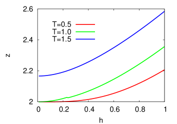
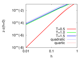
Figure 1: Left: the Lagrange multiplier $z$ as a function of the strength of the applied field $h$. Right: check of the power law approach to $z(h=0)$ for $h\to 0$ ($h^{2}$ at high and critical temperatures and $h^{2/(1-\alpha)}=h^{4}$ at low temperatures).

The magnetisation in the direction of the field, equation (7), reads in this case

$$m=\frac{h}{2}\left[z-\sqrt{z^{2}-4}\right]\;.$$

The non-linear susceptibilities can also be worked out in detail and agree with the results of the previous section in the case where $c_{0}=1/\pi$.

3.5 Phenomenology

With the aim of testing the relevance of this family of very of simple models to describe real spin-glass systems, we compare the critical exponents computed here with the ones measured experimentally by Lévy and Ogielsky [1, 2], obtained numerically by a number of authors [32], and proposed by Fisher and Huse on the basis of the droplet model [22]. In this way we try to find an optimal value of $\alpha$ to match the experimental results.

3.5.1 Comparison with experimental and numerical results.

Lévy and Ogielsky [1, 2] measured ac non-linear susceptibilities in a dilute AgMn alloy with the characteristics of a Heisenberg spin-glass in three dimensions. In their experimental studies they identified a finite critical temperature and studied the critical singularities of the nonlinear susceptibilities in the static limit.

Above $T_{c}$ Lévy and Ogielsky found

$$\chi_{3}\sim\left(\frac{T-T_{c}}{T_{c}}\right)^{-\gamma}\qquad\mbox{with}\qquad\gamma=2.3\pm 0.15\;,$$ (25)

and

$$-\frac{\chi_{5}}{\chi_{3}}\sim-\frac{\chi_{7}}{\chi_{5}}\sim\chi_{3}^{1+\beta/\gamma}\qquad\mbox{with}\qquad\beta\sim 0.9\pm 0.2\;.$$ (26)

In the spherical disordered models we found

$$\chi_{3}\sim(T-T_{c})^{\frac{-(1-\alpha)}{\alpha}}$$

so, comparison with (25) implies

$$\alpha\sim 1/3.3\sim 0.3\;.$$

In addition we found,

$$-\frac{\chi_{5}}{\chi_{3}}\sim-\frac{\chi_{7}}{\chi_{5}}\sim(T-T_{c})^{-1/\alpha}\sim\chi_{3}^{1/(1-\alpha)}\;.$$

and thus the hyperscaling relation (26) gives

$$\chi_{3}^{1+\beta/\gamma}\sim\chi_{3}^{1/(1-\alpha)}\qquad\mbox{with}\qquad\gamma=\frac{1-\alpha}{\alpha}\qquad\Rightarrow\qquad\beta=1$$ (27)

for all spherical models independently of $\alpha$ for $\alpha\in(0,1)$. Note that $\beta=1$ is consistent with the analytic behaviour of the order parameter $q_{ea}$ in the low temperature phase.

It is interesting to note that, as summarised in a recent review article [32], most isotropic spin-glasses have $\beta\sim 0.9-1.1$ and $\gamma\sim 1.9-2.3$. The first value is the one we found for all spherical models, the second one implies $\alpha\sim 0.3$. A scenario including a decoupling of spin and chiral order in Heisenberg spin-glasses has been proposed by Kawamura [33].

As for Ising spin-glasses, both experiments and simulations point to a larger value of $\gamma$. Kawashima and Rieger [32] stress that it is now well established that there is a conventional second order finite temperature transition with a diverging $\chi_{SG}$ [34, 35] and quote, basically, $\beta\sim 0.5$ and $\gamma\sim 4$ for these ‘easy-axis’ systems. Daboul, Chang and Aharony [36] estimated $\gamma$ for the Ising spin-glass model on a hypercubic lattice in $d\geq 4$ with different distributions of the coupling strengths using high temperature expansions. The values they find for higher dimensions also suggest a rather high $\gamma$ in $d=3$.

We then conclude that, as expected, the spherical model is more adequate to describe the high temperature critical behaviour of isotropic rather than Ising-like systems.

Below $T_{c}$ the dynamics are so slow that Lévy and Ogielsky could not identify a static limit in zero applied field. Aging effects come into play [37] and one has to analyse experimental, as well as numerical, data very carefully. Lévy’s data in a finite field are consistent with $\gamma^{\prime}=\gamma$, with $\gamma^{\prime}$ defined from $\chi_{3}$ which is finite below $T_{c}$ in the experimental case. The value $\alpha\sim 0.3$ that we extracted from the high $T$ analysis leads, however, to a diverging $\chi_{3}$ both in the zero applied field limit below $T_{c}$, see equation (23) obtained with (ii) $h\to 0\;\;N\to\infty$, and in the opposite order of limits, see equation (21), obtained with (i) $N\to\infty\;\;h\to 0$. Not surprisingly, spherical disordered models cannot capture all details of real spin-glasses.

3.5.2 $T<T_{c}$, comparison with the droplet model.

We now compare the critical behaviour of the spherical disordered models to that of the droplet theory of spin-glasses [22]. We shall distinguish the predictions of the latter for Ising and continuous spins.

In the Ising spin-glass phase, $T<T_{c}$, and in the limit (ii) $h\to 0$ after the thermodynamic limit $N\to\infty$, Fisher and Huse propose

$$m(h)\sim h+Ah^{d/(d-2\theta)}$$

while we have

$$m(h)\sim h+Ah^{(1+\alpha)/(1-\alpha)}\;.$$

An equivalence between the two implies

$$\alpha=\frac{\theta}{d-\theta}\;.$$ (28)

In the reversed order of limits (i) $N\to\infty\;\;h\to 0$, Fisher and Huse have

$$\chi_{3}\sim N^{1+\theta(1+\phi)}$$

and since we find $\chi_{3}\sim N$ a comparison leads to

$$\theta(1+\phi)=0\qquad\Rightarrow\qquad\theta=0\qquad\mbox{or}\qquad\phi=-1\;.$$ (29)

Using equation (28) the first option, $\theta=0$, yields $\alpha=0$. Note that $\theta=0$ is usually associated to the replica symmetry breaking scenario and it has been found numerically in $d=2$ for $J_{ij}=\pm 1$ [38].

Jönsson et al’s experimental results for the dynamic relaxation of the AgMn Heisenberg spin-glass compound analysed with the (slightly modified) droplet scaling imply $\theta\sim 1$ [39]. If we still use the relation (28) and fix $\theta=1$ we then conclude $\alpha=1/2$ (setting $d=3$). Interestingly enough, $\alpha=1/2$ corresponds to the spherical SK model but also the spherical ferromagnet in the continuum limit (the Laplacian in three dimensions leads to a density of states approaching the edge with this power).

4 Langevin Dynamics

In this section we compute the temporal behaviour of the magnetisation in the direction of the applied field as a function of time for a system quenched from infinite temperature at $t=0$. The dynamics we study is Langevin dynamics as is the case in most previous studies of the dynamics of the spherical SK model [11]-[19]

In the basis where the matrix $J$ is diagonal the stochastic evolution equations describing the Langevin dynamics of the system are

$${\partial s_{\mu}\over\partial t}=(\mu-z)s_{\mu}+h\sigma_{\mu}+\eta_{\mu}.$$ (30)

In the basis of the eigenvalues the $\sigma_{\mu}$ are again uncorrelated and of unit variance. The white noise terms have correlation function

$$\langle\,\eta_{\mu}(t)\eta_{\mu^{\prime}}(t^{\prime})\,\rangle=2T\,\delta_{\mu\mu^{\prime}}\,\delta(t-t^{\prime}).$$

The term $z$ is a dynamical Lagrange multiplier which enforces the spherical constraint and which must be calculated self-consistently. The solution to equation (30) is

$$s_{\mu}(t)=s_{\mu}(0)\;{\exp(\mu t)\over\Gamma(t)}+{\exp(\mu t)\over\Gamma(t)}\int_{0}^{t}ds\ (h\sigma_{\mu}+\eta_{\mu}(s))\;{\exp(-\mu s)\,\Gamma(s)}$$

where $\Gamma(s)\equiv\exp\left(\int_{0}^{t}ds\ z(s)\right)$. Now assuming that the initial conditions are such that they are uncorrelated with the applied field and also assuming that $\langle s_{\mu}(0)s_{\mu^{\prime}}(0)\rangle=\delta_{\mu\mu^{\prime}}$ we obtain the following equation for the magnetisation in the direction of the applied field:

$$m(t)={1\over N}\sum\sigma_{\mu}s_{\mu}(t)={h\over\Gamma(t)}\int_{0}^{t}ds\ \langle\langle\,\exp\left[\mu(t-s)\right]\,\rangle\rangle\,\Gamma(s)$$

(the field is applied at the preparation time $t=0$ and subsequently kept fixed). The self-consistent equation for $\Gamma$ is

$$\Gamma^{2}(t) = \langle\langle\,\exp(2\mu t)\,\rangle\rangle+2T\int_{0}^{t}ds\ \langle\langle\,\exp\left[2\mu(t-s)\right]\,\rangle\rangle\;\Gamma^{2}(s)$$ (31)

$$+h^{2}\int_{0}^{t}dsds^{\prime}\ \langle\langle\,\exp\left[\mu(2t-s-s^{\prime})\right]\,\rangle\rangle\;\Gamma(s)\Gamma(s^{\prime})\;.$$

We restrict out attention to the dynamical behaviour of just the linear and first non-linear susceptibilities. The above equations are thus solved perturbatively to $O(h^{3})$ to give

$$m(t) = h\int_{0}^{t}ds\ \langle\langle\exp\left[\mu(t-s)\right]\,\rangle\rangle\;{\Gamma_{0}(s)\over\Gamma_{0}(t)}$$ (32)

$$+h^{3}\int_{0}^{t}ds\ \langle\langle\exp\left[\mu(t-s)\right]\,\rangle\rangle\;{\Gamma_{1}(s)\Gamma_{0}(t)-\Gamma_{1}(t)\Gamma_{0}(s)\over\Gamma_{0}^{2}(t)}\;,$$

where $\Gamma_{0}$ obeys

$$\Gamma^{2}_{0}(t)=\langle\langle\,\exp(2\mu t)\,\rangle\rangle+2T\int_{0}^{t}ds\ \langle\langle\,\exp\left[2\mu(t-s)\right]\,\rangle\rangle\;\Gamma_{0}^{2}(s)\;,$$ (33)

and $\Gamma_{1}$ is given by

$$2\Gamma_{0}(t)\Gamma_{1}(t) = \int_{0}^{t}dsds^{\prime}\ \langle\langle\,\exp\left[\mu(2t-s-s^{\prime})\right]\,\rangle\rangle\;\Gamma_{0}(s)\Gamma_{0}(s^{\prime})$$ (34)

$$+4T\int_{0}^{t}ds\ \langle\langle\,\exp\left[2\mu(t-s)\right]\,\rangle\rangle\;\Gamma_{0}(s)\Gamma_{1}(s)\;.$$

The dynamical linear susceptibility is then

$$\chi_{1}(t)=\int_{0}^{t}ds\ \langle\langle\exp\left[\mu(t-s)\right]\,\rangle\rangle\;{\Gamma_{0}(s)\over\Gamma_{0}(t)}\;,$$ (35)

and we may write the dynamical nonlinear susceptibility as

$$\chi_{3}(t)=-6{\Gamma_{1}(t)\over\Gamma_{0}(t)}\;\chi_{1}(t)+{6\over\Gamma_{0}(t)}\int_{0}^{t}ds\ \langle\langle\exp\left[\mu(t-s)\right]\,\rangle\rangle\;\Gamma_{1}(s)\;.$$ (36)

4.1 Low temperatures

In [14] the solution of equation (33) for a general $\rho(\mu)$ in the ageing regime $T<T_{c}$ was found, this result can be compactly written as

$$\Gamma_{0}^{2}(t)=\int d\mu\ q(\mu)\exp(2\mu t)\;,$$ (37)

with $q(\mu)$ given by

$$q(\mu)={\rho(\mu)\over[1-T\chi(\mu)]^{2}}$$ (38)

and

$$\chi(\mu)=P\int d\lambda\ {\rho(\lambda)\over\mu-\lambda}\;,$$ (39)

where $P$ denotes the principal part. For the sake of completeness we re-derive the result equation (38) in a new more direct way. First if we assume the representation equation (37) we find

$$\int d\mu\ \rho(\mu)\exp(2\mu t)=\int d\mu\ q(\mu)\exp(2\mu t)$$

$$\qquad+T\int d\mu d\mu^{\prime}\,\rho(\mu^{\prime})\,q(\mu)\left[\exp(2\mu^{\prime}t)-\exp(2\mu t)\over(\mu^{\prime}-\mu)\right]\;.$$ (40)

Notice that the apparent singularity in the second integral on the right hand side at $\mu=\mu^{\prime}$ is not really present and we can replace the integral by its principal part. Equating the coefficients of $\exp(2\mu t)$ in the above equation now yields

$$q(\mu)=\rho(\mu)+T\,\chi(\mu)\,q(\mu)+T\,\rho(\mu)P\int d\mu^{\prime}\;{q(\mu^{\prime})\over\mu-\mu^{\prime}}\;.$$ (41)

The Laplace transform of equation (33) reads

$$\widetilde{\Gamma_{0}^{2}}(p)={\int d\mu\ {\rho(\mu)\over p-2\mu}\over 1-2T\int d\mu\ {\rho(\mu)\over p-2\mu}},$$

where

$$\widetilde{\Gamma_{0}^{2}}(p) \equiv \int_{0}^{\infty}dt\ \exp(-pt)\Gamma_{0}^{2}(t)=\int d\mu\;{q(\mu)\over p-2\mu}\;.$$ (42)

The above now implies that

$$P\int d\mu^{\prime}\;{q(\mu^{\prime})\over\mu-\mu^{\prime}} = {P\int d\mu^{\prime}\ {\rho(\mu^{\prime})\over\mu-\mu^{\prime}}\over 1-TP\int d\mu^{\prime}\ {\rho(\mu^{\prime})\over\mu-\mu^{\prime}}}={\chi(\mu)\over 1-T\chi(\mu)}\;.$$ (43)

Using this result for the last term in equation (41) we obtain equation (38).

4.2 The Gamma function

Let us analyse the asymptotic behaviour of $\Gamma$ in the two limits. At late times the dominant contribution to $\Gamma_{0}^{2}(t)$ comes from around $\mu=\mu_{0}$. Expanding about this point we find

$$\Gamma_{0}^{2}(t)\approx\int_{0}^{\infty}d\epsilon\ {c_{0}\epsilon^{\alpha}\over(1-T\chi(\mu_{0}))^{2}}\exp[2(\mu_{0}-\epsilon)t],$$

where we have used equation (1) for the density of states $\rho$ at the edge of the spectrum.

In what follows without loss of generality we restrict ourselves to the case where $\mu_{0}=0$ which can be achieved by a constant shift in the energy by using the interaction matrix $J^{\prime}=J-\mu_{0}I$. From the definition of $\chi(\mu)$ in equation (39) and equation (4) we find

$$\Gamma_{0}^{2}(t)\approx{c_{0}\Gamma(1+\alpha)\over(2t)^{1+\alpha}(1-{T\over T_{c}})^{2}},$$ (44)

where $\Gamma$ in the above is the standard gamma function defined as

$$\Gamma(x)=\int_{0}^{\infty}dt\ t^{x-1}\exp(-t).$$

We now compute the large time behaviour of $\Gamma$ in the region $T<T_{c}$. Notice that the Laplace transform of $\Gamma_{0}$ at small $p$ is dominated by the large $t$ behaviour of $\Gamma_{0}(t)$, for $p$ small and $\alpha<1$ we have that

$$\widetilde{\Gamma_{0}}(p)\approx A\int_{0}^{\infty}dt\exp(-pt)t^{-\frac{1+\alpha}{2}}\approx A\;\Gamma\left({1-\alpha\over 2}\right)p^{\alpha-1\over 2},$$ (45)

where $A=\sqrt{c_{0}\Gamma(1+\alpha)}2^{-(1+\alpha)/2}(1-T/T_{c})$.

In the case in which we keep the $N$ dependence, useful to study case (i), we find

$$\widetilde{\Gamma_{0}}(p)\sim\frac{1}{\sqrt{N(1-T/T_{c})}}\;\frac{1}{p-\frac{T}{N(1-T/T_{c})}}\;.$$ (46)

4.3 The linear susceptibility

Equation (35) can now be written as

$$\chi_{1}(t)={K(t)\over\Gamma_{0}(t)}\;,$$

with

$$K(t)=\int_{0}^{t}ds\;\langle\langle\,\exp\left[\mu(t-s)\right]\rangle\rangle\;\Gamma_{0}(s)\;.$$

The Laplace transform of $K$ is given by

$${\tilde{K}}(p)=\langle\langle{1\over p-\mu}\rangle\rangle\;\widetilde{\Gamma_{0}}(p)\;.$$

We may thus write

$${\tilde{K}}(p) = \left[\langle\langle-{1\over\mu}\rangle\rangle+p\;\langle\langle{1\over\mu(p-\mu)}\rangle\rangle\right]\widetilde{\Gamma_{0}}(p)$$ (47)

$$= \left[{1\over T_{c}}+p\;\langle\langle{1\over\mu(p-\mu)}\rangle\rangle\right]\widetilde{\Gamma_{0}}(p)\;.$$

(ii) $h\to 0\;\;N\to\infty$

The term $\langle\langle 1/(\mu(p-\mu))\rangle\rangle$ diverges as $p\to 0$ for $\alpha<1$; the small $p$ behaviour is thus dominated by the region around $\mu=0$. This gives for small $p$

$$\langle\langle{1\over\mu(p-\mu)}\rangle\rangle \approx -c_{0}\int_{0}^{\infty}d\epsilon{\epsilon^{\alpha}\over(p+\epsilon)\epsilon}=-c_{0}p^{\alpha-1}I(\alpha)\;,$$ (48)

where $I(\alpha)$ is as defined by equation (17). From the above and equation (45) we thus find that for small $p$

$${\tilde{K}}(p)\approx{\widetilde{\Gamma_{0}}(p)\over T_{c}}-c_{0}I(\alpha)A\Gamma({1-\alpha\over 2})p^{3\alpha-1\over 2}\;.$$

Asymptotically inverting the Laplace transform we obtain

$$K(t)\approx{\Gamma_{0}(t)\over T_{c}}-{c_{0}I(\alpha)A\Gamma({1-\alpha\over 2})\over\Gamma({1-3\alpha\over 2})t^{3\alpha+1\over 2}}$$

which finally yields for large $t$

$$\chi_{1}(t)\approx{1\over T_{c}}-{c_{0}I(\alpha)\Gamma({1-\alpha\over 2})\over\Gamma({1-3\alpha\over 2})}\;t^{-\alpha}\;.$$ (49)

We thus see that $\chi_{1}(t)$ decays to its low temperature equilibrium value with a power law $t^{-\alpha}$. Interestingly the coefficient of this decaying term is negative for $\alpha<1/3$, meaning that $\chi_{1}(t)$ achieves its equilibrium value from below, whereas for $\alpha>1/3$ the coefficient is positive and thus $\chi_{1}(t)$ achieves its equilibrium value from above.

(i) $N\to\infty\;\;h\to 0$

In this limit one can analyse $\widetilde{K}(p)$ in (47) keeping the $1/N$ contributions. One finds

$$\chi_{1}(t)=\frac{1}{T}-\left(\frac{1}{T}-\frac{1}{T_{c}}\right)\;e^{-\frac{t}{N(\beta-\beta_{c})}}\;.$$

Note that if we set $t/N\ll 1$ we recover $\chi_{1}\sim\beta_{c}$.

4.4 The non-linear susceptibility

We now turn to the results for the nonlinear susceptibility $\chi_{3}$. If we define $Q(t)=\Gamma_{0}(t)\Gamma_{1}(t)$, from equation (34) we find that the Laplace transform of $Q$ obeys

$$\widetilde{Q}(p)={\widetilde{f}(p)\over 1-2T\langle\langle\,{1\over p-2\mu}\,\rangle\rangle}\;,$$

where

$$f(t)={1\over 2}\int_{0}^{t}dsds^{\prime}\ \langle\langle\exp\left[2\mu t-\mu s-\mu s^{\prime}\right]\,\rangle\rangle\;\Gamma_{0}(s)\Gamma_{0}(s^{\prime})\;.$$

(ii) $h\to 0\;\;N\to\infty$

Let us now focus on this order of limits. Making the substitution $w=-\mu t$ and $s=vt$ we find

$$f(t)={1\over 2}\int_{0}^{-\mu^{*}t}\rho\left({-w\over t}\right){dw\over t}\left[\int_{0}^{1}tdv\ \exp\left[-w(1-v)\right]\;\Gamma_{0}(vt)\right]^{2}.$$

We now use the asymptotic form of $\Gamma_{0}$ in equation (44) to find, for large $t$,

$$f(t)\approx{A^{2}c_{0}\over 2t^{2\alpha}}\int dw\;w^{\alpha}\left[\int_{0}^{1}dv\;{\exp\left[-w(1-v)\right]\over v^{1+\alpha\over 2}}\right]^{2}\;.$$

Thus $f(t)=B^{\prime}/t^{2\alpha}$ for large $t$ and one may verify that the constant $B^{\prime}$ is finite for $\alpha<1$. Consequently, we obtain

$$\Gamma_{1}(t)=B\;t^{\frac{1}{2}(1-3\alpha)}\;.$$

The small $p$ behaviour of the Laplace transform of $\Gamma_{1}$ is thus given by

$$\widetilde{\Gamma_{1}}(p)\approx B\;\Gamma\left({3\over 2}(1-\alpha)\right)p^{-{3\over 2}(1-\alpha)}\;.$$

We now rearrange the result in equation (36) as

$$\chi_{3}(t)=-6\;{\Gamma_{1}(t)\over\Gamma_{0}(t)}\left[\chi_{1}(t)-{1\over T_{c}}\right]-6\;{L(t)\over\Gamma_{0}(t)}$$

where

$$L(t)={\Gamma_{1}(t)\over T_{c}}-\int_{0}^{t}ds\ \langle\langle\,\exp\left[\mu(t-s)\right]\,\rangle\rangle\;\Gamma_{1}(s)\;.$$

The Laplace transform of $L$ is given by

$${\tilde{L}}(p)=\left({1\over T_{c}}-\langle\langle{1\over p-\mu}\,\rangle\rangle\right)\;\widetilde{\Gamma_{1}}(p)=-p\;\widetilde{\Gamma_{1}}(p)\langle\langle{1\over\mu(p-\mu)}\,\rangle\rangle\;.$$ (50)

For small $p$ using the asymptotic result for $\Gamma_{1}$ and equation (48) we find

$${\tilde{L}}(p)\approx c_{0}\,B\,I(\alpha)\;\Gamma\left({3\over 2}(1-\alpha)\right)p^{{5\over 2}\alpha-{3\over 2}}\;,$$

which implies that the late time behaviour of $L$ is

$$L(t)\approx{c_{0}\,B\,I(\alpha)\;\Gamma\left({3\over 2}(1-\alpha)\right)\over\Gamma({3\over 2}-{5\over 2}\alpha)\;t^{{5\over 2}\alpha-{1\over 2}}}\;.$$

We can compute the other contribution to $\chi_{3}$ using the asymptotic result for $\chi_{1}$ equation (49) to obtain the result

$$\chi_{3}(t)\approx-{6\,c_{0}\,B\,I(\alpha)\over A}\left[{\Gamma\left({3\over 2}(1-\alpha)\right)\over\Gamma({3\over 2}-{5\over 2}\alpha)}-{\Gamma({1-\alpha\over 2})\over\Gamma({1-3\alpha\over 2})}\right]t^{1-2\alpha}.$$

We therefore see that when $\alpha<1/2$ the nonlinear susceptibility diverges as $\chi_{3}(t)\approx Ct^{1-2\alpha}$. When $\alpha>1/2$ $\chi_{3}(t)$ decays to zero as $1/t^{2\alpha-1}$. These dynamical results are of course in agreement with the static calculations carried out earlier. The coefficient of this term is determined by the sign of that in the square brackets, the first prefactor being negative. Numerical evaluation of the factor in square brackets confirms that it is positive for $\alpha\in(0,1)$ and thus the dynamical nonlinear susceptibility is negative. Indeed for $T>T_{c}$ the static value is negative and the dynamical calculation confirms the divergence to an infinite negative value for $\alpha<1/2$.

(i) $N\to\infty\;\;h\to 0$

In order to compute $\chi_{3}(t)$ we need to compute $\Gamma_{0}(t)$ and $\Gamma_{1}(t)$ keeping the correction to the leading exponential in time terms. From equations  (34) and (46) we find

$$\Gamma_{0}(t) \sim \frac{1}{\sqrt{N\left(1-T/T_{c}\right)}}\;e^{\frac{t}{N(\beta-\beta_{c})}}\;,$$ (51)

$$\Gamma_{1}(t) \sim \frac{1}{2T^{2}}\sqrt{N\left(1-T/T_{c}\right)}\;\left\{1+2t/[N(\beta-\beta_{c})]\right\}\;e^{\frac{t}{N(\beta-\beta_{c})}}\;.$$ (52)

Using equation (36) it can be verified that the asymptotic limit of $\chi_{3}(t)$ is the static value (21) up to a correction term that decays exponentially as $e^{-\frac{t}{N(\beta-\beta_{c})}}$.

5 Discussion and Conclusions

We have studied in detail the linear and first non-linear susceptibilities of generalised random orthogonal model spherical spin glasses. Their physics is completely determined by the density of states of the two body interaction matrix. In particular the exponent, $\alpha$ describing how the density of states vanishes at the upper edge, determines completely the critical behaviour at the phase transition and the dynamical evolution of $\chi_{1}(t)$ and $\chi_{3}(t)$ in the limit (ii) considered here where the limit $h\to 0$ is taken after the limit $N\to\infty$ in the computations. With respect to the Gaussian $p=2$ spin glass model we see that the existence of the parameter $\alpha$ gives us the possibility to carry out a more meaningful comparison between the model and experimental and droplet scaling theories. An interesting aspect of this work is that it clearly demonstrates the possibility that $\chi_{3}$ may appear to be finite for certain classes of model (with $\alpha\geq 1/2$) if the applied fields used to carry out the measurements place us in the regime of limits (ii). However it is in this same region where the cusp in the linear susceptibility exists. These results, though for a somewhat idealised mean field model, could well have some bearing on the interpretation of susceptibility and magnetisation measurements in disordered and frustrated spin systems [40]. Finally we have mentioned that the models considered here will still exhibit a finite temperature transition in the presence of an external magnetic field if $\alpha>1$. In this case it is the higher oder ($n>3$) susceptibilities which will diverge and it will be interesting to study, in particular, the dynamics of these models.

References

- [1] L. P. Lévy and A. T. Ogielski, Phys. Rev. Lett. 57 3288 (1986).
- [2] L. P. Lévy, Phys. Rev. B 38, 4963 (1988).
- [3] S. Nair and A. K. Nigam, cond-mat/0509360.
- [4] S. Franz and G. Parisi, J. Phys. C 12, 6335 (2000). C. Donati, S. Franz, S. Glotzer, and G. Parisi, J. Non-Cryst. Solids, 307, 215 (2002).
- [5] J-P Bouchaud and G. Biroli, Phys. Rev. B 72, 064204 (2005).
- [6] C. Toninelli, M. Wyart, L. Berthier, G. Biroli, and J-P Bouchaud, Phys. Rev. E 71, 041505 (2005).
- [7] L. Berthier, G. Biroli, J-P Bouchaud, W. Kob, K. Miyazaki, and D. Reichman cond-mat/0609656 and cond-mat/0609658.
- [8] C. Chamon, M. P. Kennett, H. Castillo, and L. F. Cugliandolo, Phys. Rev. Lett. 89, 217201 (2002). H. Castillo, C. Chamon, L. F. Cugliandolo, and M. P. Kennett, Phys. Rev. Lett. 88, 237201 (2002). H. Castillo, C. Chamon,L. F. Cugliandolo, and M. P. Kennett, Phys. Rev. B 68, 134442 (2003). C. Chamon, P. Charbonneau, L. F. Cugliandolo, D. R. Reichmann, and M. Sellitto, J. Chem. Phys. 121, 10120 (2004). C. Chammon, L. F. Cugliandolo and H. Yoshino, J. Stat. Mech. (2006) P01006.
- [9] P. Mayer, P. Sollich, L. Berthier, and J. P. Garrahan, J. Stat. Mech. P05002 (2005).
- [10] T. H. Berlin and M. Kac, Phys. Rev. 86, 821 (1952). H. W. Lewis and G. H. Wannier, Phys. Rev. 88, 682 (1952). H. W. Lewis and G. H. Wannier, Phys. Rev. 90, 1131E (1953). M. Lax, Phys. Rev. 97 1419 (1955). C. C. Yan and G. H. Wannier, J. Math. Phys. 6, 1833 (1965). M. Kac and C. J. Thompson, J. Math. Phys. 18, 1650 (1977).
- [11] J. M. Kosterlitz, D. J. Thouless, and R. C. Jones, J. Phys. C 36, 1217 (1976).
- [12] P. Shukla and S. Singh, Phys. Rev. B 23, 4661 (1981).
- [13] S. Ciuchi and F. de Pasquale, Nucl. Phys. B 300, 31 (1988).
- [14] L. F. Cugliandolo and D. S. Dean, J. Phys. A 28, 4213 (1995). The relevant expression is equation (A.3) but note the change in notation, in the current paper corresponds to in this reference.
- [15] L. F. Cugliandolo and D. S. Dean, J. Phys A: Math. Gen. 28, L453 (1995).
- [16] W. Zippold, R. Kuehn, H. Horner, Eur. Phys. J. B 13, 531 (1999).
- [17] M. Campellone, P. Ranieri, G. Parisi, Phys. Rev. B 59, 1036 (1999).
- [18] L. L. Bonilla, F. G. Padilla, G. Parisi and F Ritort, Phys. Rev. B 54, 4170 (1996).
- [19] L. Berthier, L. F. Cugliandolo, and J. L. Iguain, Phys. Rev. E 63, 051302 (2001).
- [20] G. Semerjian, L. F. Cugliandolo, and A. Montanari, J. Stat. Phys. 115, 493 (2004).
- [21] G. Semerjian and L. F. Cugliandolo, Europhys. Lett. 61, 247 (2003).
- [22] D. S. Fisher and D. A Huse, Phys. Rev. B 38, 386 (1988).
- [23] H. Yoshino and T. Rizzo, Step-wise reponses in mesoscopic glassy systems: a mean-field approach, cond-mat/0608293.
- [24] S. Kirkpatrick and A. P. Young, J. App. Phys. 52, 1712 (1981).
- [25] A. P. Young, A. J. Bray, and M. A. Moore J. Phys. C 17, L149 (1984).
- [26] C. Monthus, J. Phys. A: Math. Gen. 36, 11605 (2003).
- [27] C. Chatelain, J. Phys. A 36, 10739 (2003).
- [28] F. Ricci-Tersenghi, Phys. Rev. E 68, R065104 (2003).
- [29] E. Lippiello, F. Corberi, and M. Zannetti, Phys. Rev. E 71, 036104 (2005).
- [30] R. Cherrier, D. S. Dean, and A. Lefèvre, Phys. Rev. E 67, 046112 (2003).
- [31] E. Marinari, G. Parisi and F. Ritort, J. Phys. A (Math. Gen.) 27, 7647 (1994).
- [32] N. Kawashima and H. Rieger, in “Frustrated Spin Systems”, H.T.Diep ed. (World Scientific, Singapore, 2005) and references therein.
- [33] H. Kawamura, Spin-chirality decoupling in Heisenberg spin glasses and related systems, at ICM2006 conference, to appear in J. Mag. Mag. Mater, cond-mat/0609652.
- [34] M. Palassini and S. Caracciolo, Phys. Rev. Lett. 82, 5128 (1999).
- [35] H. G. Ballesteros, A. Cruz, L. A. Fernandez, V. Martin-Mayor, J. Pech, J. J. Ruiz-Lorenzo, A. Tarancon, P. Tellez, C. L. Ullod and C. Ungil, Phys. Rev. B 62, 14237 (2000).
- [36] D. Daboul, I. Chang and A. Aharony, Eur. Phys. J. B 41, 231 (2004)
- [37] E. Vincent, J. Hammann, M. Ocio, J-P Bouchaud, and L. F. Cugliandolo in Complex behaviour of glassy systems, E. Rubi ed. (Springer-Verlag, Berlin, 1997).
- [38] J. Lukic, A. Galluccio, E. Marinari, O. C. Martin, and G. Rinaldi, Phys. Rev. Lett. 92, 117202 (2004).
- [39] P. E. Jönsson, H. Yoshino, P. Nordblad, H. Aruga-Katori, and A. Ito, Phys. Rev. Lett. 88, 257204 (2002).
- [40] W. Bisson and A. S. Wills, cond-mat/0608234. M. Suzuki and I. S. Suzuki, cond-mat/0601561. A. K. Kundu, P. Nordblad, and C. N. R. Rao, Phys. Rev. B 72, 144423 (2005).